SOCIAL-ECOLOGICAL IMPACTS OF CHINA’S PAYMENTS FOR ECOSYSTEM
SERVICES PROGRAMS ON LAND USE, MIGRATION AND LIVELIHOODS
Qi Zhang
A dissertation submitted to the faculty at the University of North Carolina at Chapel Hill in
partial fulfillment of the requirements for the degree of Doctor of Philosophy in the Department
of Geography.
Chapel Hill
2017
Approved by:
Conghe Song
Richard Bilsborrow
Xiaodong Chen
Pamela Jagger
ii
©2017
Qi Zhang
iii ABSTRACT
QI ZHANG: Social-ecological impacts of China’s Payments for Ecosystem Services Programs on land use, migration and livelihoods
(Under the direction of Conghe Song)
iv
v
ACKNOWLEDGEMENTS
vi
TABLE OF CONTENTS
LIST OF TABLES ... ix
LIST OF FIGURES ... x
INTRODUCTION ... 1
IMPACTS OF PAYMENTS FOR ECOSYSTEM SERVICES ON CROPLAND ABANDONMENT ... 5
2.1 Introduction ... 5
2.2 Methods... 9
2.2.1 Study area ... 9
2.2.2 Household survey and fieldwork ... 11
2.2.3 Statistical analyses ... 12
2.3 Results ... 13
2.3.1 Temporal dynamics of cropland abandonment ... 13
2.3.2 Reasons for cropland abandonment ... 15
2.3.3 Statistical modeling of cropland abandonment ... 17
2.4 Discussion ... 20
2.5 Conclusions ... 23
IMPACTS OF PAYMENTS FOR ECOSYSTEM SERVICES ON OUT-MIGRATION ... 25
3.1 Introduction ... 25
3.2 Theories on migration ... 28
3.3 Study area ... 30
3.4 Research questions and hypotheses ... 33
vii
3.6 Sampling design ... 35
3.7 Analytical and statistical methods ... 37
3.8 Results and Discussion ... 41
3.8.1 Temporal trend ... 41
3.8.2 Descriptive analysis ... 44
3.8.3 Determinants of out-migration: multivariate results ... 48
3.8.4 Interpreting the marginal effects ... 53
3.9 Conclusions ... 54
IMPACTS OF PAYMENTS FOR ECOSYSTEM SERVICES ON RURAL LIVELIHOODS ... 58
4.1 Introduction ... 58
4.2 Materials and methods ... 61
4.2.1 Study area ... 61
4.2.2 Data acquisition, entry and preparation ... 63
4.2.2.1 Household survey ... 63
4.2.2.2 Data estimation and imputation ... 63
4.2.3 Income levels and sources ... 64
4.2.4 Income inequality and income generation ... 66
4.2.4.1 Gini coefficient ... 66
4.2.4.2 Determinants of income generation and inequality... 68
4.3 Results and Discussion ... 70
4.3.1 Income levels and sources ... 70
4.3.2 Contributions of different sources of income and income inequality ... 75
4.3.3 Determinants of household income and income inequality ... 79
4.4 Conclusions ... 84
CONCLUSIONS... 86
viii
ix
LIST OF TABLES
Table 2.1 Statistical summary of areas for parcels in use and parcels abandoned (n=1202). ... 14 Table 2.2 Statistical summary and t-test of mean values for parcel-level
variables between parcels in use and parcels abandoned (n=1202). ... 18 Table 2.3 Statistical summary of household-level variables for households surveyed (N=249). ... 18 Table 2.4 Fixed effects (odds ratios) and random effect estimation of parcel
features and household characteristics on cropland abandonment
(number of parcels = 1202, number of households = 249). ... 20 Table 3.1 Description of independent variables for modeling out-migration. ... 39 Table 3.2 Mean values of individual-level variables for non-migrants and
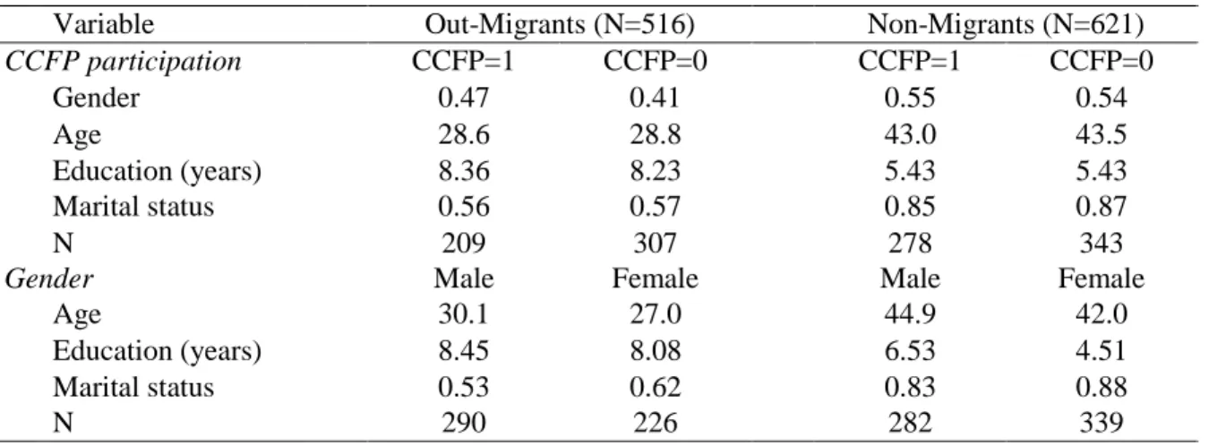
out-migrants aged 15-59 at the time of migration/non-migration, by
CCFP participation and by gender. ... 45 Table 3.3 Means, standard deviations, minimum and maximum values of
variables for non-migrants and out-migrants aged 15-59 in Tiantangzhai Township (asterisks indicate when differences between migrants and
non-migrants are statistically significant). ... 47 Table 3.4 Results (odds ratios and marginal effects) for determinants of
out-migration from the random effects model. ... 50 Table 4.1 Statistics on per capita income and income shares from different
sources for households with and without CCFP (asterisks indicate
when differences in means are statistically significant). ... 71 Table 4.2 Statistics on farm costs, animal and forest resources for households
participating in CCFP and not participating (asterisks indicate when
differences in means are statistically significant). ... 74 Table 4.3 Measures of inequality attributed to different income sources for
households with and without CCFP. ... 78 Table 4.4 Marginal effects of income sources for households with and without CCFP ... 79 Table 4.5 Interpretation of independent variables with means and standard deviation. ... 80 Table 4.6 Factors determining the generation of income and the contribution
x
LIST OF FIGURES
Figure 2.1 Study area: 2013 Landsat OLI image in true color (RGB=432)
for Tiantangzhai Township in Anhui, China... 10 Figure 2.2 Temporal changes of survival rates based on individual cropland
parcels for households with and without of the CCFP from 2003 to 2013. The log-rank test of the equality of the two survival functions by the year of 2013: Chi2=0.03, Pr>Chi2=0.873. However, the log-rank test reveals significant differences of the two survival rates during 2009-2011 with
p-values below 0.01. ... 14 Figure 2.3 Percentage of reasons for cropland abandonment by households with
and without CCFP in four time periods: a) the entire time period,
b) Year 03-07, c) Year 08-11, and d) Year 12-13.Y-axis is the percentage of the reasons for cropland abandonment provided by respondents. X-axis is the category of responses. R1, lack of labor due to migration or aging; R2, crop raiding by wild animals; R3, too far away from the house; R4, not worthwhile for cropping due to high opportunity cost; R5, lack of reliable water supply for crop growth; R6, frequent natural disasters such
as flooding, drought, insects, and disease. ... 16 Figure 3.1 Study area: Tiantangzhai Township in Anhui, China ... 31 Figure 3.2 Proportion of household members aged 15-59 out-migrating each year
during 2000-14 for (panel 1) households with and without CCFP; (panel 2) households receiving EWFP payments above and below the mean. The asterisk for 2014 indicates that data were available only for the first half of 2014 since the survey was carried out in July 2014. The height of the
observation for 2014 is annualized to be comparable with other years. ... 42 Figure 3.3 Personal attributes of gender, age, education and marital status for
non-migrants and out-migrants aged 15-59. The y-axis is the percentage of individuals. Black histogram bars indicate out-migrants, and white
bars indicate non-migrants. ... 46 Figure 4.1 Annual net income of different sources for rural households (all
households), households participating in the CCFP (CCFP=1) and
households not participating (CCFP=0). The x-axis is denotes the income source. ... 71 Figure 4.2 Distribution of sources of income of households with and without
CCFP, for low-, medium- and high-income groups. The X-axis denotes the income source and the y-axis the share of income. The asterisk
indicates that the sources of household income are statistically significantly
different at the 5% level (only for medium income households). ... 73 Figure 4.3 Lorenz Curves and Gini coefficients of total net income for households
1 CHAPTER 1 INTRODUCTION
For the first time in human history, there are more than seven billion people now living on the Earth with over half of them in the cities. The total population of the world is projected to be 9.6 billion by 2050 and 10.9 billion by 2100 (Cohen, 2003; Gerland et al., 2014). The land needed for food production and development, the natural resources needed for economic growth have never been greater. The human inhabitance of the planet Earth has brought in tremendous impacts on the environment, inducing the global climate change and threatening the welfare of future generations (Goudie & Viles, 2013). Thus, there is an urgent need to understand the interactions between human activities and environmental changes so that timely policies can be put in place to make essential ecosystem goods and services sustainable for future generations.
2
behavior in response to the degraded land may cause further environmental changes, influencing the provision of environmental services. The changing land, in turn, can feedback to the human society, influencing humans’ behavior in adaptation to the environmental change. Thus, land use change is the key to the problems raised from complex interactions between human and the environment across multiple scales (Verburg, 2014).
To address the adverse problems in the human-environment nexus, Payment for Ecosystem Services (PES) has emerged as an incentive-based approach to conserve the environment through direct investment (S Wunder, Engel, & Pagiola, 2008). Under a PES scheme, a voluntary transaction flows from buyers to providers, with the latter securing the provision of ecosystem services. PES programs often link to land use and target land parcels owned by farm households in rural areas (X. Chen, Lupi, Viña, He, & Liu, 2010). Thus, PES programs are usually designed with goals in both environmental conservation and rural poverty alleviation. Due to the dual goals, the success of environmental policies under PES schemes depends on whether such programs are sustainable in a long run. Therefore, empirical evaluation of PES programs on their ecological and social outcomes is needed to inform policy-makers with regard to the sustainability of PES programs.
3
Liu, 2006). The Conversion of Cropland to Forest Program (CCFP), which is the largest PES program, has received great attention in the world due to its large scale and potentially huge impacts (J. Liu, Li, Ouyang, Tam, & Chen, 2008). The CCFP, also known as the “Grain-for-Green” (GFG) program, encourages farmers to convert their cropland on sloping areas and otherwise ecologically sensitive areas to forests or grasslands, and compensates the participating households based on the land areas enrolled (Conghe Song et al., 2014). The ultimate goals of the CCFP are soil and water conservation through forest restoration and poverty alleviation in the rural areas. A second forest program is the Ecological Welfare Forest Program (EWFP), which is a forestry policy for classification-based forest management. The initiation of the EWFP ties to natural reserve, aiming at preserving natural forests for sustainable environmental goods and services as part of the welfare for the public (Dai, Zhao, Shao, Zhou, & Tang, 2009). Under the EWFP, farm households who owned natural forests receive compensation from the government in return for giving up timber harvesting privilege for commercial purposes. Thus, the EWFP is essentially a PES program.
4
households, the overall improvement of livelihood is limited. Bennett et al. (2014) highlighted trade-offs between searching off-farm jobs and managing reforested areas for rural households participating in the programs. Given mixed results from studies of policy evaluation, the Chinese government still faces challenges of maintaining sustainable provision of ecosystem services from the PES programs and the improvement of rural livelihoods at the same time. The PES programs in China have existed for over ten years, there is still lack of systematic and integrated evaluation of the PES programs in terms of their social and ecological impacts.
5 CHAPTER 2
IMPACTS OF PAYMENTS FOR ECOSYSTEM SERVICES ON CROPLAND ABANDONMENT
2.1 Introduction
Land-cover and land-use change (LCLUC) has profound impacts on vital ecosystem goods and services across the world (DeFries, Foley, & Asner, 2004; Kareiva, Watts, McDonald, & Boucher, 2007). Land cover has been transformed tremendously by human beings through land use practices (Foley, 2005). Two dominant forms of the transformation are agricultural expansion and deforestation (Geist & Lambin, 2002; Lambin, Geist, & Lepers, 2003). Recently, land use transitions have occurred as new patterns of LCLUC across the world associated with the economic development (Lambin & Meyfroidt, 2011). Under the circumstance of urbanization and economic development, farmers in rural areas migrate to cities to seek better off-farm opportunities. The loss of labor impels rural households to abandon their marginal cropland (T. K. Rudel et al., 2009). As a result, cropland abandonment has occurred as a prominent manifestation of land use transitions under the pathway of economic development.
6
have abandoned their cultivation in the uplands with low productivity as a result of agricultural intensification in the lowlands (Meyfroidt & Lambin, 2008).
Cropland abandonment creates a reverse transformation from human-dominated fields to the land surface with less human impact. This reverse process has multiple ecological impacts on the environment. The abandoned land, followed by natural succession to grass or secondary-forests (T. K. Rudel, 2010), offers the potential of increasing carbon storage (Silver, Ostertag, & Lugo, 2000; Kuemmerle et al., 2011), reducing runoff and soil erosion (Jiao et al., 2007; Y. Liu, Fu, Lü, Wang, & Gao, 2012), and restoring of forest ecosystems (Bowen, McAlpine, House, & Smith, 2007; Chazdon, 2008). Cropland abandonment has socioeconomic consequences, such as global food provision and rural labor allocation. Studies observed a remarkable amount of cropland abandonment across the world, making the cultivated land become increasingly scarcer resource for food production to the growing population (Ramankutty, Foley, & Olejniczak, 2002; Lambin & Meyfroidt, 2011). Land abandonment also influences households’ behavior in livelihood strategies. In the Nepalese Himalaya, for example, the abandonment of cultivated fields caused food shortage in villages, and forced households to seek opportunities for non-farm jobs via out-migration (Khanal NR and Watanabe T, 2006). Given the effects on both environmental conservation and social development, understanding determinants of cropland abandonment is important in advancing the knowledge of land use transitions.
7
be associated with a lower likelihood of cropland abandonment due to the need for food production. However, the involvement of non-agricultural activities, such as off-farm work, raising domestic animals and migration, may reduce farm labor availability, leading to a high probability of cropland abandonment. Demographical properties, such as the household head’s age, gender and education, may also be important factors influencing cropland abandonment, although their effects vary (Daniel Müller & Munroe, 2008). For example, higher education increases the chance of getting off-farm jobs, but one with higher education may also be equipped with technology (e.g., irrigation) to expand cropland. The socioeconomic factors on cropland abandonment are sometimes intertwined with political changes, particularly the intervention of environmental policies (Mitsuda & Ito, 2011). Thus, cropland abandonment often coincides with the intervention of environmental policies when policy-makers employed policy instruments, such as area protection and Payment for Ecosystem Services (PES) programs, to trigger and/or accelerate land use transitions (T. K. Rudel et al., 2005; Sierra & Russman, 2006). Recently, PES has emerged as an innovative approach to enhance ecosystem services. However, the relationship between the PES programs and cropland abandonment are not well understood.
China is the largest developing country by the population in the world. Historically, China was constantly under the pressure to produce enough food to feed its large population. A nationwide movement was initiated by the central government in the 1950s to reclaim wasteland to become cropland (Ye, Fang, Ren, Zhang, & Chen, 2009). Since the adoption of reform and open policies in the late 1970s, China’s economy has witnessed a double-digit growth for three decades. Such rapid economic growth offered unprecedented opportunities for the rural residents to work in the cities with much better payment than farming. More than two hundred million people migrated from the remote, rural areas to the cities, seeking better economic opportunities in China (Z. Liang, 2016). The rising rural population mobility was inevitably followed by a land-use trend of cropland abandonment in marginal areas, as observed in other countries (Busch, 2006; López, Bocco, Mendoza, Velázquez, & Rogelio Aguirre-Rivera, 2006; Grau & Aide, 2007).
8
2009). Most of the new forest programs are implemented under the scheme of the Payment for Ecosystem Services (PES). In many cases, PES programs link to land use change, where landowners voluntarily provide environmental benefits through land use management such as preserving existing forests and establishing forests on barren or other non-forest lands (Engel, Pagiola, & Wunder, 2008; Pattanayak, Wunder, & Ferraro, 2010). One of the conservation policies is the Ecological Welfare Forests Program (EWFP), which was implemented with logging bans, aimed at protecting natural forests to stave off ecosystem degradation (Dai et al., 2009). Commercial logging is prohibited for EWFP forests while local residents who own natural forests receive subsidies for giving up timber harvesting privilege. Thus, the EWFP is essentially a PES program.
Among the PES programs, the China’s Conversion of Cropland to Forest Program (CCFP) has received great attention due to its large-scale impacts on forest rehabilitation (J. Liu et al., 2008). The CCFP, implemented around 2002, is the world’s largest PES program, whereby households who enroll their cropland into the program receive compensation from the central government based on the areas reforested. These croplands are usually located on steep slopes or otherwise in ecologically sensitive areas. Since the implementation of the CCFP, official statistics from the State Forestry Administration have revealed a substantial increase in forest cover. By 2013, over 9.2 million ha of cropland in total have been enrolled into the CCFP (Sate Forestry Administration, 2014). As the first round of the CCFP will end soon, China State Council approved the initiation of the second round CCFP. Policy-makers have planned to convert additional 0.6 million ha cropland to forests (Sate Forestry Administration, 2015).
9
land-use practices in mountainous areas, where land parcels are most likely to be targeted and enrolled into the CCFP. Understanding the underlying factors that influence farmers’ decision on cropland abandonment can provide critical information to policy-makers for targeting qualified land parcels and designing the payment schemes for the PES programs. Thus, the present study uses a case study in Tiantangzhai Township, Anhui Province, China, to explore the underlying determinants of cropland abandonment under the CCFP and EWFP.
2.2 Methods
2.2.1 Study area
The study area, Tiantangzhai Township, is located in the eastern part of the Dabieshan Mountain in western Anhui Province, China (Fig. 2.1). The region falls in the northern edge of subtropical climate zone, covering an area of 189 km2, with elevation varying from about 400 to 1,650 meters above sea level. The mean annual temperature is 16.4℃ and the annual total precipitation is 1,350 mm (Conghe Song et al., 2014). The area is remote from major development within a county that is recognized as a county in poverty by the central government. The climate condition makes the area favorable for vegetation growth and thus natural forests dominate the landscape in this region. The township also forms part of the Tianma Nature Reserve with well-developed tourism, protecting the last remaining primary forests in eastern China (Han, Fang, & Huang, 2011). Under the Nature Reserve, natural forests are protected and designated as ecological welfare forests (i.e., EWFP forests) in the middle 1990s. In return, the government compensates the households that own EWFP forests at a rate of 131.25 Yuan/ha/year. Although commercial logging is banned, subsistence use of wood is allowed, such as fuelwood collection.
10
the main tree species for the CCFP in this area is sweetgum (Liquidambar styraciflua) while economic forests are very limited. The CCFP compensation rate in the study area was set by the central government at 3,450 Yuan/ha/year during the initial contract period. The initial contract lasted for 8 years for ecological forests. The central government renewed their initial contracts for another 8 years, but at a lower compensation rate of 1,875 Yuan/ha/year.
Figure 2.1 Study area: 2013 Landsat OLI image in true color (RGB=432) for Tiantangzhai Township in Anhui, China
11
those for subsistence grain production, were not allowed to be abandoned according to state regulations. After the Household Responsibility System (HRS), all collective land parcels were allocated to individual households (Mullan, Grosjean, & Kontoleon, 2011). Although the ultimate land owner is the state, farmers enjoy a high degree of usufructuary rights under the current land tenure system. For example, village leaders rarely adjust the holdings of private parcels, and farmers have rights to lease or rent land parcels, to choose which crop to grow, and even to fallow or abandon land parcels. Two primary types of land parcels have been found in this mountainous region: paddy land and dryland. Paddy-land parcels are mainly used for rice, while dryland parcels are for dryland crops such as corn, potatoes and wheat.
2.2.2 Household survey and fieldwork
12
parcels were of interest. In addition, households were also asked about the abandonment reason for each abandoned parcel. Based on respondents’ answers, six major reasons were categorized for cropland abandonment: R1, lack of labor due to migration or aging; R2, crop raiding by wild animals; R3, too far away from the house; R4, not worthwhile for cropping due to high opportunity costs; R5, lack of reliable water supply for crop growth; R6, frequent natural disasters such as flooding, drought, insects, and diseases. Having parcel information recorded, a fieldwork is carried out to measure geographic coordinates of each land parcel using global positioning system (GPS) units. Geographic coordinates were recorded for the approximate center for each land parcel because of the limited amount of time to delineate the boundary for each land parcel in the field. Overlaying the coordinates with the digital elevation model (DEM), biophysical properties (e.g., elevation, topographic wetness index (TWI), and aspect) of each land parcel are derived. Moreover, the nearest distances of each parcel to the edge of both natural forests and CCFP forest stands classified are also calculated based on satellite images (Q. Zhang, Hakkenberg, & Song, 2016). The natural forest cover is classified based on the 2002 satellite image before the establishment of CCFP forest stands.
2.2.3 Statistical analyses
The temporal trend of cropland abandonment is captured by estimating cumulative probabilities of survived land (i.e., land parcels that had not been abandoned) for each year since 2002. The probability curves (Goel, Khanna, & Kishore, 2010) are depicted for households with and without CCFP. The equity of the curves for the two groups is tested with the log-rank statistic to track the difference of abandonment rates between the two groups. For the abandoned parcels, the percentage of each category of abandonment reasons provided by respondents are tallied for the two types of households in four time periods: Year 03-13, Year 03-07, Year 08-11, and Year 12-03-13, with the last three periods corresponding to different stages of CCFP implementation.
13
nested across various levels (Pan & Bilsborrow, 2005; Y. Zhang et al., 2014). For example, land use decision is influenced by biophysical characteristics at the parcel level and socioeconomic characteristics at the household level and farming activities among different land parcels within the same households are more similar than between households. Thus, a random-coefficient logit model (Guo & Zhao, 2000) is used to examine both fixed effects of parcel/household features and random effects among households on cropland abandonment. The dependent variable of the model is whether the land parcel had been abandoned (=1) or under cultivation (=0) by the time of the survey. In this model, the coefficients of explanatory variables are estimated with a random intercept and fixed slopes. The random coefficient multilevel model is expressed in Equation (2.1).
log ( Pr(𝑌𝑖𝑗 = 1)
1 − Pr(𝑌𝑖𝑗 = 1)) = 𝛽0+ ∑ 𝛽𝑝𝑋𝑖𝑗𝑝 𝑃
𝑝=1
+ ∑ 𝛾𝑞𝑍𝑗𝑞 𝑄
𝑞=1
+ 𝜇𝑗+ 𝜀𝑖𝑗 (2.1)
where Pr(Yij= 1) is the probability of the abandonment of the ith parcel owned by the jth household. Further,
Xijp is the pth predictor describing parcel features and Zjq is the qth predictor of the jth household characteristics that influence land abandonment on parcels. The intercept is captured by the coefficients β0, while fixed effects at the parcel level and the household level are captured by the parameters βp and γq corresponding to Xijp and Zjq, respectively. Finally, εij and µj capture the random effects at the parcel level and the household level, respectively.
2.3 Results
2.3.1 Temporal dynamics of cropland abandonment
14
the abandonment rate of land parcels for CCFP households almost equals that for non-participants at the time of interview.
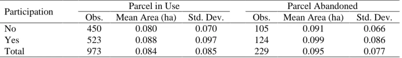
Table 2.1 Statistical summary of areas for parcels in use and parcels abandoned (n=1202).
Participation Parcel in Use Parcel Abandoned
Obs. Mean Area (ha) Std. Dev. Obs. Mean Area (ha) Std. Dev.
No 450 0.080 0.070 105 0.091 0.066
Yes 523 0.088 0.097 124 0.099 0.086
Total 973 0.084 0.085 229 0.095 0.077
Figure 2.2 Temporal changes of survival rates based on individual cropland parcels for households with and without of the CCFP from 2003 to 2013. The log-rank test of the equality of the two survival functions by the year of 2013: Chi2=0.03, Pr>Chi2=0.873. However, the log-rank test reveals significant differences of the two survival rates during 2009-2011 with p-values below 0.01.
15
Therefore, the survival rate monotonically decreases as more cropland parcels are abandoned. The overall survival rate of land parcels for CCFP households is higher than that of parcels for non-CCFP households before 2013. However, the two trend lines converges by 2013, leading to an insignificant difference between the two types of households. This converging trend suggests an acceleration of cropland abandonment near the time of interview by households that are participating in the CCFP.
2.3.2 Reasons for cropland abandonment
16
Figure 2.3 Percentage of reasons for cropland abandonment by households with and without CCFP in four time periods: a) the entire time period, b) Year 03-07, c) Year 08-11, and d) Year 12-13.Y-axis is the percentage of the reasons for cropland abandonment provided by respondents. X-axis is the category of responses. R1, lack of labor due to migration or aging; R2, crop raiding by wild animals; R3, too far away from the house; R4, not worthwhile for cropping due to high opportunity cost; R5, lack of reliable water supply for crop growth; R6, frequent natural disasters such as flooding, drought, insects, and disease.
17
of long walking distance, which is nearly as important as lack of labor for non-CCFP households, while making trivial contribution for CCFP households. During the last period of 2012-13, lack of labor, high opportunity costs and lack of reliable water supply make the dominant contributions to cropland abandonment for CCFP households, while other reasons have little effects. Again the reasons for cropland abandonment for non-CCFP households remain diverse, with lack of labor, crop raiding and lack of water as the dominant factors, while high opportunity costs and frequent natural disasters continue to contribute to cropland abandonment.
2.3.3 Statistical modeling of cropland abandonment
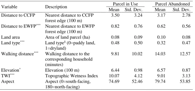
At the parcel level, there are significant differences in biophysical properties between abandoned parcels and parcels in use (Table 2.2). Overall, abandoned parcels have significantly higher elevations, lower TWI values, and longer distances to the owners’ houses. In addition, dryland parcels account for a significantly lower proportion of abandoned parcels than paddy-land parcels. However, the mean area and the aspect of abandoned parcels do not significantly differ from those of parcels in use. The nearest distances of abandoned parcels to EWFP and CCFP forests are shorter than those of parcels in use.
18
Table 2.2 Statistical summary and t-test of mean differences for parcel-level variables between parcels in use and parcels abandoned (n=1202).
Variable Description Parcel in Use Parcel Abandoned
Mean Std. Dev. Mean Std. Dev. Distance to CCFP Nearest distance to CCFP
forest edge (100 m)
3.50 3.24 3.17 2.78
Distance to EWFP*** Nearest distance to EWFP forest edge (100 m)
0.82 0.76 0.62 0.56
Land area Area of land parcel (ha) 0.08 0.09 0.10 0.08
Land type*** Land type§ (0=paddy land, 1=dryland)
0.48 0.50 0.32 0.47
Walking distance*** Walking distance to the corresponding household (minutes)
9.81 10.02 14.03 12.57
Elevation* Elevation (100 m) 6.44 0.98 6.57 0.87
TWI*** Topographic Wetness Index 10.07 4.12 9.01 3.13
Aspect Aspect (0=south-facing, 180=north-facing)
74.69 52.46 79.74 53.85
* p < 0.05; ** p < 0.01; *** p < 0.001
§ “Land type” is a categorical variable and the mean is the proportion of the observations whose choice is “dryland” (=1).
Table 2.3 Statistical summary of household-level variables for households surveyed (N=249).
Variable Description Mean Std. Dev.
CCFP payment Conversion of Cropland to Forest Program subsidy (1,000 yuan)
0.17 0.24 EWFP payment Ecological Welfare Forest Program subsidy (1,000 yuan) 0.35 0.41
Age Age of household head 52.48 9.62
Gender§ Gender of household head (0=male, 1=female) 0.05 0.21
Education Education of household head (years) 6.95 2.71
Farm labor Number of non-migrants (i.e., people who live at home, being able to provide farm labor) aged 18-60
1.79 1.09
Total land Amount of total land owned (ha) 0.47 0.23
Crop raiding§ If suffered crop raiding by wildlife without effective actions (0=no, 1=yes)
0.41 0.49
Raising pigs§ If has pigs (0=no, 1=yes) 0.73 0.45
Local off-farm Proportion of local off-farm income to the total gross income 0.35 0.37
Fuelwood Fuelwood usage per year (1,000 kg) 8.86 5.90
19
Results from the random-coefficient multilevel logit model reveal significant fixed effects of parcel features and household characteristics on cropland abandonment (Table. 2.4). Although the parcel area does not have significant effects on cropland abandonment, land types experience different abandonment rates. Dryland parcels are 74% less likely to be abandoned than paddy-land parcels. Parcels located in adverse conditions are more likely to be abandoned. For example, for every additional walking minute the likelihood of abandonment increases by 5%, while an additional unit of TWI decreases the likelihood of abandonment by 8%. TWI is a proximate measure for soil moisture based on the slope and the areas flowing into a given unit area (Sørensen, Zinko, & Seibert, 2006). The larger the TWI value is, the higher the soil moisture might be. However, the elevation and aspect do not have significant effects on cropland abandonment. In addition, the nearest distances of parcels to EWFP and CCFP forests have significant effects on cropland abandonment. Every additional 100m distance to EWFP and CCFP forests decrease the probability of abandonment by 47% and 8%, respectively.
20
Table 2.4 Fixed effects (odds ratios) and random effect estimation of parcel features and household characteristics on cropland abandonment (number of parcels = 1202, number of households = 249).
Variables Odds Ratio (Std. Err.) z P>|z| Distance to CCFP 0.92 (0.04) -2.04 0.0410* Distance to EWFP 0.53 (0.10) -3.26 0.0010**
Land area 0.23 (0.34) -1.01 0.3140
Land type 0.26 (0.06) -5.70 0.0000***
Walking distance 1.05 (0.01) 4.53 0.0000***
Elevation 1.06 (0.16) 0.40 0.6890
TWI 0.92 (0.03) -2.81 0.0050**
Aspect 1.00 (0.00) 1.58 0.1150
EWFP payment 2.01 (0.65) 2.15 0.0320*
CCFP payment 0.71 (0.45) -0.54 0.5870
Age 0.99 (0.01) -0.63 0.5260
Gender 1.01 (0.63) 0.02 0.9870
Education 0.97 (0.05) -0.61 0.5410
Farm labor 0.75 (0.10) -2.05 0.0410*
Total land 1.31 (0.91) 0.39 0.6990
Crop raiding 1.31 (0.33) 1.06 0.2880
Raising pig 0.50 (0.15) -2.35 0.0190*
Local off-farm 2.36 (0.85) 2.37 0.0180*
Fuelwood 1.02 (0.02) 0.76 0.4500
Constant 1.10 (1.69) 0.06 0.9490
Constant variance 1.33 (0.41) Intra-class correlation 0.29 (0.06) * p < 0.05; ** p < 0.01; *** p < 0.001
The log-ratio test shows that the Chi2 value is 31.30 with p-value 0.000.
2.4 Discussion
21
their cropland abandoned. Previous studies found that the EWFP encouraged household members rely on off-farm activities instead of forest resources (Jiang, Jiang, Liu, Yu, & Wang, 2002).
There is a significant difference of land parcel survival rates between households with and without CCFP during 2009-2011, but the cropland survival trend lines of the two types of households converge by 2013. According to Fig. 2.3d, lack of labor, high opportunity costs and lack of reliable water supply are the primary reasons for cropland abandonment for CCFP households during 2012-13. This implies the increase of opportunity costs for farming as a result of overall economic development in China. The convergence of the cropland abandonment rates between CCFP and non-CCFP households indicates the additionality of forest areas gained from the CCFP. The CCFP in China is a well-known PES program, where households are incentivized or “persuaded” to retire their marginal cropland parcels for forest restoration (Bennett, 2008; S Wunder et al., 2008; Conghe Song et al., 2014). Land parcels that are located on steeper slopes and/or in ecologically-sensitive areas have the priority to be targeted by the local government. Having these poorly-accessible parcels enrolled into the program, participating households are less likely to abandon their remaining land parcels in the years immediately after the CCFP implementation. As time goes on, the increase in forest areas due to the CCFP and EWFP may cause more crop raiding by wildlife, dampening crop yield for the remaining land parcels adjacent to forests (X. Chen, Zhang, Peterson, & Song, 2017). This also explains that the proximity of cropland parcels to EWFP and CCFP forest edges is associated with a high probability of being abandoned (Table 2.4).
22
ownership of CCFP forests as well as the right of CCFP land management. After the enrollment of their land, CCFP households need to manage the newly-establish trees for the survivorship (Bennett et al., 2014) and thus they cannot spare labor for off-farm work during the early years. When the trees grew up and required fewer management actions, households tended to allocate more labor to off-farm activities. This may explain the convergence of cropland abandonment for the two types of households.
The effects of PES programs on cropland abandonment are examined together with biophysical determinants and household socioeconomic drivers. The results show the importance of topographic conditions (e.g., topographic wetness index, TWI) and geographic accessibility (i.e., the walking distance from the house to land parcels), which is consistent with findings in other areas of the world (D Müller et al., 2009; Lakes, Müller, & Krüger, 2009; Sikor et al., 2009; Daniel Müller, Leitão, & Sikor, 2013). The TWI, which is often included in land cover transition models (Rutherford, Bebi, Edwards, & Zimmermann, 2008), contains information of both water accumulation and slopes. An area with higher TWI is associated with better water availability and a moderate slope, thus a more suitable environmental condition for cultivation, particularly on paddy land with rice farming (Y. Li & Barker, 2004).
23
The study on cropland abandonment offers useful information in evaluating the cost-effectiveness of the CCFP, which is essential for the design of such PES programs in the future (Sven Wunder, 2007; Engel et al., 2008). In the CCFP, two interrelated aspects of the cost-effectiveness are the payment scheme and land parcel targeting (Y. Chen, Yang, Sweeney, & Feng, 2010). The Chinese government adopted a two-tier payment scheme for the CCFP: a higher payment for croplands enrolled in the CCFP in the Yangtze River Basin than those in the Yellow River Basin. This is believed to be less cost-effective than a discriminative payment scheme based on opportunity costs (Ferraro, 2008; Y. Chen et al., 2010). Despite the difficulty of estimating opportunity costs, enrolled parcels are likely to have low costs of forgoing cultivation (i.e., opportunity costs) if they possess high risks of being abandoned. Targeting such parcels with less payment can minimize the cost of similar programs in the future. In addition, the abandoned land by households would turn to natural landscape such as grassland or shrubs/forests given sufficient time, potentially providing ecosystem services even without the implementation of environmental policy, albeit at a slower rate (Silver et al., 2000). Actually, scholars have recently reported the prevalence of cropland abandonment in mountainous areas, calling for the need of further consideration of the expansion of the CCFP (X. Li, Tan, & Xin, 2014). Future research may involve the analyses of a time series of data to better capture how the participation of the CCFP, intertwined with other drivers, has affected cropland abandonment through time. Understanding the process of cropland abandonment can provide useful information to the policy makers on designing similar programs in the future.
2.5 Conclusions
24
25 CHAPTER 3
IMPACTS OF PAYMENTS FOR ECOSYSTEM SERVICES ON OUT-MIGRATION
3.1 Introduction
Rural out-migration is an on-going process accompanying socio-economic development in the developing world (Stark & Bloom, 1985; Findley, 1987; R E Bilsborrow, McDevitt, Kossoudji, & Fuller, 1987; E. J. Taylor, 1999). China, as the most populous developing country, is no exception. Since the adoption of the Reform and Opening-up Policy in 1978, China’s economy has witnessed double-digit growth for three decades, which has led to unprecedented opportunities for residents in the countryside. More than 200 million people have moved from rural areas to cities, seeking better economic opportunities (NBS, 2012; Z. Liang, 2016). The annual population flow on an unprecedented scale substantially alters the demographic and economic landscape via population redistribution (Cai & Wang, 2003; Fan, 2003). Such great mobility also has profound impacts on Chinese society. As a result, the study of rural out-migration in China is of ever growing interest to both out-migration scholars and policy-makers.
26
The hukou institution was imposed by the central government in the 1950s as a principal mechanism to keep rural residents from seeking livelihoods in cities, reducing pressures on government budgets to provide infrastructure and welfare for urban residents (Chan & Zhang, 1999). For example, a farmer born in the countryside with an agricultural hukou registration was not allowed to reside or work permanently in a big city. However, the Reform and Opening-up Policy adopted by the Chinese government created a huge need for labor in urban areas. Therefore the Chinese government relaxed control over population mobility from rural areas, allowing rural migrants to seek temporary employment in urban areas (Cai & Wang, 2003). Thus, a large number of rural people, typically with low education, migrated to fill labor needs in the cities (Sun & Fan, 2011). These migrants, characterized as the floating population, have come to change jobs easily and frequently from city to city and from year to year, although some return to the original location where their hukou is located (Z. Liang & Ma, 2004). Given this complex behavior of out-migration in rural China, empirical studies on the determinants of migration are needed to better understand the causes and mechanism of population redistribution and its implications for socio-economic development.
The dynamics of rural out-migration is closely tied to the dynamics of the natural environment, which is referred to as the migration-environment nexus (Carr, 2005; Laczko, Aghazarm, & Bilsborrow, 2009; Richard E. Bilsborrow & Henry, 2012). Among all the environmental conditions, land use and land management has been recognized as the key linkage between the migration decision-making of rural populations and environmental change (Braimoh, 2004; R. Chen, Ye, Cai, Xing, & Chen, 2014). For example, early rural residents who migrated out from places of origin in response to degraded land may subsequently degrade the land elsewhere in their areas of destination, which may cause further migration in a chain process (Charnley, 1997). The behavior of out-migrants has also been viewed as an adapting strategy by rural farmers coping with high risks of crop failure under adverse and unpredictable environmental conditions (Ellis, 2003; Konseiga, 2007). The migration-environment relationship is thus of crucial importance for regional planning on both the environment and human society.
27
land use change (Engel et al., 2008; Pattanayak et al., 2010). In the late 1990s, China adopted the PES approach in the new forest policies in response to the devastation from natural disasters caused primarily by land use change (J. Liu et al., 2008). The largest PES program is the Conversion of Cropland to Forest Program (CCFP), which was implemented in 25 of the 31 provinces, of China starting around 2000, involving 32 million rural households and costing RMB 430 billion yuan (Bennett et al., 2014; Yin, Liu, Zhao, Yao, & Liu, 2014). Under the CCFP, farmers reforest their cropland located on moderately steep slopes or otherwise ecologically-sensitive areas in return for a cash payment from the central government based on the areas reforested. A second PES program, the Ecological Welfare Forest Program (EWFP), is a forest management program for natural forests, which aims to preserve existing forests by prohibiting commercial logging (Dai et al., 2009). Thus the government provides cash compensation to farmers for giving up commercial logging privilege based on the area in natural forests owned by farmers, mostly in mountainous areas. At the same time, the central government abolished all land taxes on these owned forests. To facilitate conservation, when the land use policies of Mao based on collectively owned farmland and land in natural forests were replaced in the 1980s with long-term private ownership, both farmland and forest lands were distributed to the households living on them.
28
possible time-lags in the effects of the PES programs on household livelihood strategies. As the CCFP and EWFP have existed since 2000, it is now time to investigate their possible medium-term impacts on rural out-migration, ultimately to better understand their socio-economic consequences and develop appropriate policies.
The present research thus aims to understand the roles played by the Chinese PES programs (i.e., CCFP and EWFP) in rural out-migration using a case study of Tiantangzhai Township, Anhui Province. Since migration decisions of rural farmers may also be affected by various personal and household characteristics and contextual factors, these drivers must also be taken into account to isolate the effects of PES policies on out-migration. The specific objectives of this study thus include: 1) tracking temporal trends in the out-migration of households during the implementation of the PES programs, and 2) developing a statistical estimation model to examine the effects of the PES programs and other factors on out-migration. Since the PES approach is being adopted around the world as a major tool for environmental restoration, the results of this present study should be useful for understanding other PES programs in other countries besides China and therefore provide useful inputs for policy-makers designing similar PES programs in the future.
3.2 Theories on migration
29
decision-making of migration by individuals is conceptualized as a function of expected return and expected cost of moving (Sjaastad, 1962; Schwartz, 1976). In these models, key elements affecting the migration decision are individual characteristics relating to human capital, such as age, gender, education, occupation and work experience and skills, and marital status. For example, a person with higher education and work skills expects a higher salary in the destination with better opportunities, while an individual beyond the peak productivity age can expect a lower return. Despite the importance of personal characteristics, these individual-based models ignore the fact that migration decisions are also often affected by household strategies at the household level and household conditions and resources (De Jong & Gardner, 1981; Lauby & Stark, 1988; Root & De Jong, 1991).
30
live initially (with the previous out-migrant) in the destination location (Richard E Bilsborrow, Oberai, & Standing, 1984; Massey, 1990).
Beyond individual and household factors that may influence migration decisions are community-level factors, which may influence migration behavior as contextual conditions (Richard E Bilsborrow et al., 1984; Findley, 1987; T. Rudel & Roper, 1997). Such contextual factors include labor markets and wage levels, accessibility to transportation, land and other resources, availability of particular kinds of infrastructure (e.g., hospitals, schools), and other socio-economic conditions. Taking into account such areal factors in migration models provides a more comprehensive understanding on the factors that may influence migration decision.
3.3 Study area
The study area is in Tiantangzhai Township, located in a mountainous region in western Anhui Province (Fig. 3.1). The township covers an area of 189 km2 and lies at an elevation ranging from 402 m to 1,651 m above sea level. Tiantangzhai has a mild climate albeit with rough terrain, suitable for abundant forest cover. The township is remote from the county capital (Jinzhai County) and the provincial capital, Hefei, and the county is recognized as a county in poverty by the Chinese government. This township also forms part of the Tianma Nature Reserve in the eastern Dabieshan Mountains, protecting the last remaining primary forests in eastern China. Due to the rich natural resources (including waterfalls, stunning views, and mountain trails), part of the reserve has been developed into an important ecotourism area, providing local residents with business opportunities.
31
potatoes) on their own small land parcels. Before the land reforms, land parcels were collectively managed by so-called resident groups, with only small pieces of land allocated to individual households in the same group (G. Li et al., 1998). But under the rural reform policy in the 1980s, all the land was divided among the households in the resident group, which is a cluster of 10 to 40 households. There are currently 165 resident groups in the township. Households within the same resident group sometimes still share cropland and farm together but mostly work their own land under 99 year leases from the government.
Figure 3.1 Study area: Tiantangzhai Township in Anhui, China
32
rugged terrain, most planted trees are ecological trees, mainly sweetgum (Liquidambar styraciflua). For ecological forests, the payment scheme was the same as that of the Yangtze River Basin: 230 Yuan/mu/year (1 mu =1/15 ha) for the first 8-year contract (2000-2008), which was cut to half (125 Yuan/mu/year) for the second 8-year contract (Conghe Song et al., 2014).
The township is also part of an area where a separate forest conservation policy was implemented. Under the nature reserve, natural forests are designated as ecological welfare forests. The Ecological Welfare Forest Program (EWFP) was hence created by the Chinese government for managing natural forests. Because of the high forest cover in the study area, almost every household owns some natural forests, but the area varies widely. Farmers received 8.75 Yuan/mu/year as compensation for forgoing commercial logging of their natural forests. Although commercial timber harvesting is prohibited, subsistence use of the forest resources is allowed.
33 3.4 Research questions and hypotheses
Based on the migration theories and understanding of the study area from multiple visits, the study here investigates rural out-migration in Tiantangzhai Township by asking the following research questions: What are the levels of out-migration, and the characteristics of migrants compared to non-migrants? What are the driving factors that influence individuals’ out-migration decisions? What are the effects of the PES programs on this out-migration? To answer these questions, the study develops an empirical model of the determinants of out-migration to test hypotheses about various potentially influential factors. It is hypothesized that the migration decision of an individual is affected by personal attributes, household characteristics and contextual factors at the community level.
At the individual level, it is hypothesized that out-migrants tend to be relatively young, single, educated and male as these attributes are more favored by employers in urban areas. However, females who are single may also be associated with a high likelihood of migration since they are less restricted by family matters than those who are married. At the household level, the human capital of the household head is hypothesized to have influence on the migration decisions of other household members, because it is associated with more access to information and awareness of opportunities elsewhere, and higher aspirations for children. Accessibility of the house to the township center and previous migration experience of any household member other than the person in question is hypothesized to positively influence migration as each decreases migration costs. Household size itself may be positively associated with individual out-migration since a large household size is more likely to have surplus labor, controlling for farm size. The amount of land a household has and the areas engaged in cropland cultivation or raising animals are hypothesized to be negatively associated with out-migration since they offer opportunities for work to household members.
34
either the CCFP or EWFP may be positively related to out-migration by providing financial support. The elevation of the household is also included, though this is likely to have some collinearity with the access variables in this mountainous setting. Finally, at the contextual or community level, accessibility of the community to a hospital and a primary school is hypothesized to be negatively related to migration because it reduces the incentive to migrate to gain easier access to schools or health care. Thus the lack of a close school or health facility (as well as of other community infrastructure) may serve as “push” factors.
3.5 Data sources
The study draws on data collected primarily from a household survey conducted in Tiantangzhai Township in the summer of 2014. A fairly comprehensive questionnaire with 22 sections was designed to obtain socio-economic data at the individual and household level, on demographic characteristics, land available and agricultural activities, household living conditions, participation in PES programs (i.e., EWFP and CCFP), etc. Households participating and not participating in the CCFP program were both sampled and interviewed for the comparison of the two groups, as described above.
35
only the out-migrant but also a randomly-selected non-migrant (when available) in the migrant household pertaining to the time of migration of the household migrant. In survey households with no out-migrant over the period—less than half—data were collected for a randomly selected non-migrant aged 15-59 pertaining to his/her situation five years prior to the survey, or near to the midpoint of migration of the migrants observed. This is about the best that can be done to create an appropriate comparison population of non-migrants, and is an important contribution of the project methodology as it contrasts with the universal practice to date of collecting data for non-migrants only pertaining to the time of the survey. This is evidently not appropriate since the at-risk group of non-migrants not migrating when others did is the population of non-migrants available at the time of migration of the migrants1.
In addition to the household survey, a survey at the community (i.e., resident group) level was conducted using a structured questionnaire. The resident group leader(s) were interviewed for each resident group sampled in the household survey, to obtain information resident group size (i.e., number of households) and geographic factors such as accessibility to the nearest hospital/clinic and primary school.
3.6 Sampling design
Due to fact that the proportion of households in the CCFP in the study region is low (about 17%), disproportionate random sampling is used in order to generate a sample with roughly similar numbers of households participating in the CCFP and not participating. This is a key part of the project methodology and is not common in field surveys, which overwhelmingly tend to select households with equal probabilities of selection. But that is very inefficient when one is interested in particular kinds of households and data are available in a sampling frame to identify those households—in this case, households with and without CCFP. Such a sampling frame was indeed available, as the county forestry office provided data on the names of all household heads, their resident group, and whether they are receiving or not CCFP. A two-stage sampling strategy is adopted, with the first two-stage being communities (i.e., resident groups) and the
1 See Bilsborrow et al. (1984, 1997) and Bilsborrow (2016). This continues to be an issue in the design of migration
36
second stage, households. Based on the availability of human and financial resources and estimated costs of fieldwork, the goal of the household survey was set to interview approximately 500 households, without replacement of absent or refusing households since that all-too-common practice distorts the principle of probability sampling which requires that the a priori probability of selection of each household be known before doing the fieldwork. The selection of households needed to take into account knowledge gained from a prior, smaller survey in the same general study region which found that many households were not available due to the whole household having out-migrated to live elsewhere or the lack of an adequate respondent due to temporary absence (or in a few cases to old-age senility of the remaining adult(s) living in the sampled dwelling). Accordingly, the original goal was to select a sample of about 750 households in order to obtain complete data from a sample of around 500 households, taking into account the expected problems above as well as normal refusals and incomplete responses.
Based on the average number of households in a resident group and the dispersion of resident groups, it is estimated that the number of resident groups to be sampled should be 40, both to reach the total number of households in the sample (750) and to ensure a broad geographic distribution of households in the study area. It is also estimated that a team of five interviewers could, contact about 20 households per day, completing about 13 on average. Therefore, the sampling approach first selected 40 resident groups out of the total 165, and then selected up to 20 households from each sampled resident group.
37
sample resident group in the stratum, i.e., the ratio of the total number of resident groups in a stratum to the number sampled resident groups.
At the second sampling stage, a maximum of 20 households from each of the 40 sampled resident groups was selected. For resident groups that had fewer than 20 households, all households were selected. For households with more than 20 households, 10 households were randomly select representing CCFP households and non-CCFP households. If one of the two types of households had fewer than ten households, all were selected, and additional households would be randomly selected from the other group comprising the remaining households to make it a 20 household sample in total. For example, if a resident group has 30 households, with 25 enrolled in CCFP and 5 not enrolled, the 20 household sample size would include all 5 households that were not enrolled in CCFP, and an additional 15 households randomly selected from the 25 CCFP households. Each household sampled in a resident group therefore carries a resident group weight for its type (CCFP or non-CCFP), which depends on both the number of households of its type in its resident group and the number successfully interviewed. The weights are calculated as the ratio of the number of total households in a resident group to the number successfully interviewed, separately for CCFP and non-CCFP households in each resident group (see Table A3.2 in Appendix for details). The final result of this sampling process, and the actual fieldwork, was that the team of interviewers successfully interviewed 481 households, 56% participating in the CCFP, yielding data for 1957 individuals in total.
3.7 Analytical and statistical methods
38
individuals aged 15-59 at some time in the study period and at risk of out-migration, with nearly half (589) out-migrating at some time in the interval. The reason for including 2000-02 is to show the prevailing level of out-migration right before the implementation of PES policies. The temporal trends of out-migration were compared between 1) households participating in CCFP and those not, and 2) households receiving EWFP payment above the average and those below the average (470 Yuan per household), since virtually all households in the sample received some EWFP payment.
39
Table 3.1 Description of independent variables for modeling out-migration.
Variable Description
Individual-level
Gender 0=male, 1=female
Age Age in years
Education Whether finished primary school (0=no, 1=yes)
Marital status§ Marital status (0=single, divorced or widowed; 1=married) Single female Interaction term of gender and marital status
Household (HH)-level
CCFP payment Compensation received from CCFP in past 12 months (1,000 yuan) EWFP payment Compensation received from EWFP in past 12 months (1,000 yuan) Gender of HH head 0=male, 1=female
HH Head’s age Age of household head in years
HH Head’s education Whether household head finished primary school (0=no, 1=yes) HH Head’s marital status 0=single, divorced or widowed, 1=married
Elevation House elevation above sea level (meters)
Walking distance Walking distance to nearest paved road measured by time (minutes) Household size Number of people living in household
Household wellness Wellness index of household (score range 3-33) Cultivated land Total area of land under cultivation (mu)
Previous migration Whether any current member who aged 15+ of household has previous out-migration experience (0=no, 1=yes)
Animal sale Whether household has any income from selling domestic animals in past 12 months (0=no, 1=yes)
Local off-farm work Whether any household member was engaged in local off-farm employment in past 12 months (0=no, 1=yes)
Use forest resources Whether household extracted forest resources, such as herbal medicines, in past 12 months (0=no, 1=yes)
Community (RG)-level
Community size Number of households in resident group
Distance to school Distance to nearest primary school measured in walking time (minutes)
Distance to hospital Distance to nearest hospital or clinic measured in walking time (minutes)
§ Single individuals (=0) includes those who are single, divorced or widowed at the time of reference; however, divorced and widowed made up a trivial proportion of the total.
40
age, education) and household characteristics (e.g., number of people in the household) but also contextual factors at the community level (e.g., distance to the nearest school). Thus, a multilevel model is appropriate for capturing the nested relationships of individual out-migration decisions being made based on a hierarchy of individual, household, and community factors.
In this study, the dependent variable is whether an individual migrated out (=1) or not (=0) in a given year. As the dependent variable is dichotomous, logistic regression is used for parameter estimation. Independent variables examined at the individual level are personal attributes, viz., gender, age, education and marital status. An interaction term of gender and marital status (i.e., single female) is also included to examine if there is an interaction effect of gender and marital status—to capture if there is an effect beyond the direct effects of gender and marital status.
Variables at the household level include attributes of the household head (i.e., gender, age, education and marital status), size of farm land area, household elevation and walking distance to the nearest paved road, household size, household wellness, and whether any other (current or former) member of the household had migrated away previously. The model also includes variables reflecting household engagement (that is, of any member) in any of several main types of livelihood activities in the 12 months prior to the interview, including whether sold animals, whether engaged in local off-farm work, and whether extracted forest resources. The effects of PES programs are modeled based on the amount of payment received by the household from the CCFP and EWFP in the past 12 months.
Potentially relevant variables collected at the resident group or community level include community size and accessibility to facilities such as hospitals and primary schools. The form of the model used is expressed in Equation (3.1).
𝑀𝑖𝑗𝑘 = 𝑓(𝐼𝑖𝑗𝑘, 𝐻𝑗𝑘, 𝐶𝑘) (3.1)
41
Equation (3.1). Note also that the model is estimated based on 1,137 individuals aged 15-59 for some years and exposed to the risk of out-migration during 2003-14. Apart from age, which is tracked for each person, and household size, which varies with out-migration and return migration (and occasional deaths), the model implicitly assumes that the characteristics of the individual, household and community as recorded at the time of the survey in 2014 did not change over time, except for the key individual and household characteristics specifically obtained in the questionnaire pertaining to the time of migration2. In fact, it is known that one key variable, total land (in crops, in forest) available to the household rarely changed over time, since the government allocated fixed amounts to households with long-term (99 year) leases, and households, even when members leave including all members, make sure some relative stays behind to continue to lay claim to the land for the household, to retain its hukou or legal household registration (Y. Zhu, 2007). The list of independent variables at each level with detailed descriptions is presented in Table 3.1. Note that all data at the individual/household level are weighted in the multivariate model.
3.8 Results and Discussion
3.8.1 Temporal trend
A graph showing the percentage of persons in households with and without CCFP exposed to the risk of out-migration (aged 15-59) who out-migrated in each year shows out-migration to be generally increasing over time during 2000-13 (Fig. 3.2, top panel). Looking at the annual fluctuations for the CCFP households (solid) line, there is a moderate increase immediately after 2002 when the CCFP was first implemented, followed by a second surge in 2010 when the first 8-years of registration was completed, and people could register for a second 8-year participation in CCFP. The larger apparent increase after 10 years of the implementation of the CCFP in 2013 is likely due partly to respondents remembering and reporting out-migration better in the most recent year. The dip in 2008 might be due to the impact of the global economic recession.
42
43
The interpretation now moves on to compare the two lines on the probabilities of out-migration from households with and without the CCFP, still in the top panel. On the one hand, the proportion of out-migrants from CCFP-participating households was overall higher than that from households not participating after 2002. During 2009-10, however, the out-migration rate from CCFP households increased and reached a small peak while the rate from non-CCFP households remained the same. This may be due to households receiving the modest CCFP payment recovering more quickly from the economic recession. However, both groups had a sharp increase in out-migration in 2012-2013, which might be linked to a major rural economic stimulus program3 of the central government. There was a huge surge in real estate development from the stimulus, attracting rural labor for construction.
The lower panel of figure 3.2 provides a prima facie assessment of whether the amount of money received by households from the second PES program, the Ecological Welfare Forest Program (EWFP), has had any evident effect on stimulating or not out-migration. Since all households received EWFP compensation, the comparing analysis examined whether those receiving more than the average were more likely to have out-migrants than those receiving less than the average. The two almost parallel lines suggest the difference is small, but that those receiving more were in general less likely to have out-migrants, though this was also true prior to the PES program in 2000-2002. Thus the difference in out-migration rates is the opposite to that of CCFP payments. This is probably because households who received more compensation from the EWFP are more satisfied with rural living conditions and thus less likely to send out-migrants. Another key difference between EWFP and CCFP is that EWFP has no impact on freeing farm labor as does the CCFP, by taking cultivable land out of cultivation to reforest it.
3 The State Council of the People's Republic of China announced the economic stimulus plan on 9 November 2008