doi:10.1017/S0305004114000371 First published online 14 August 2014
357
Canonical heights and division polynomials
BYROBINDEJONG
Mathematisch Instituut, Universiteit Leiden, PO Box9512,2300RA Leiden, The Netherlands.
e-mail:[email protected]
ANDJ. STEFFEN M ¨ULLER
Institut f¨ur Mathematik, Carl von Ossietzky Universit¨at Oldenburg, 26111Oldenburg, Germany.
e-mail:[email protected]
(Received26June2013;revised26June2014)
Abstract
We discuss a new method to compute the canonical height of an algebraic point on a hyperelliptic jacobian over a number field. The method does not require any geometrical models, neither p-adic nor complex analytic ones. In the case of genus 2 we also present a version that requires no factorisation at all. The method is based on a recurrence rela-tion for the ‘division polynomials’ associated to hyperelliptic jacobians, and a diophantine approximation result due to Faltings.
1. Introduction
In [3] G. Everest and T. Ward show how to approximate to high precision the canon-ical height of an algebraic point on an elliptic curve E over a number field K with a limit formula using the (recurrence) sequence ofdivision polynomialsφn associated to E, and a diophantine approximation result.
The φn have natural analogues for jacobians of hyperelliptic curves. In [18] Y. Uchida shows how to obtain recurrence relations for theφnfor hyperelliptic jacobians of dimension
g 2. Further there exists a suitable analogue of the diophantine approximation result employed by Everest and Ward, proved by G. Faltings [4]. In this paper we derive a limit formula for the canonical height of an algebraic point on a hyperelliptic jacobian from these inputs.
2. Statement of the main results
LetK be a number field with ring of integersOK and let(X,o)be a pointed hyperelliptic curve of genusg2 overK given by an equationy2 = f(x)with f ∈O
K[x]monic of odd degree 2g+1, whereois the unique point at infinity. LetJdenote the jacobian variety ofX. Then the theta divisoronJ is the reduced and irreducible divisor onJ whose support is given by the set of all points which can be represented by a divisor(p1)+ · · · +(pd)−d(o), where all pi ∈ X andd < g. Equivalently, these are precisely the points whose reduced Mumford representation(a(x),b(x))(cf. Section 5) satisfies deg(a) < g.
For each integern 1 there exists a canonical ‘division polynomial’φn in the function field ofJ overK, see Section 5. We have
divφn = [n]∗−n2 .
For each place v of K we further have a canonical local height function λv, see [18, section 7]. These functions are determined by the key relations:
log|φn(p)|v = −λv(np)+n2λv(p)
for each integern1, each placevand generic p∈ J(Kv), where|·|vis the absolute value onKv, normalized as in Subsection 3·2.
Let p be a point in J(K), not in supp(). Leth: J(K) → R be the canonical height with respect to the canonical principal polarization onJ. We have the formula:
[K: Q]h(p)= v
nvλv(p) ,
wherenvis a standard local factor defined in Subsection 3·2. Put
T(p)= {n∈Z>0|np^supp()}.
Then one can show thatT(p)is an infinite set.
Our first result extends [3, theorem 3] and gives a limit formula for the canonical local heightλv in terms of the division polynomials. The proof is based on a diophantine approx-imation result due to Faltings (Theorem 4·1).
THEOREM2·1. Letvbe any place of K and let p∈ J(K)\supp()be a rational point. Then T(p)is an infinite set and the formula
λv(p)= lim
n→∞ n∈T(p)
1
n2 log|φn(p)|v
holds.
LetSbe a finite set of places ofK. We put:
hS(p)= 1
[K:Q] limn→∞ n∈T(p)
1 n2 log
v∈S
|φn(p)|nvv.
Theorem 2·1 implies that the limithS(p)exists, and gives theS-part of the canonical height of p.
THEOREM2·2. Assume that p is a point in J(K), not insupp(). Then the limithS(p)
exists, and the formula
[K :Q]hS(p)=
v∈S
nvλv(p)
holds.
Our next result expressesh(p)in terms ofhS(p)andhS(2p), for a suitable setS. Let= 24gdisc(f)denote the discriminant ofX. Then the curveX, and hence the jacobian J, has good reduction outside the set Sbadof places ofK dividing the ideal(). LetS∞be the set of archimedean places ofK.
THEOREM2·3. Let p ∈ J(K)and assume that both p and2p are not insupp(). Let S be a finite set of places of K containing SbadS∞, such that for allv ^ S one has that neither p nor2p lies on the theta divisor modulov. Then the formula
h(p)= −1
3hS(p)+ 1 3hS(2p) holds.
Note that, for a finite placevoutsideSbad, saying that plies on the theta divisor modulovis
equivalent to saying that pcan be represented by a divisor(p1)+ · · · +(pg)−g(o), where one of the pi reduces toomodulov, or that one of the coefficients of the first polynomial in the Mumford representation of pis notv-integral. We will see thathS(p)andhS(2p)are effectively computable forSandpas in Theorem 2·3.
Forg=2 we can prove a simpler version of Theorem 2·3.
THEOREM2·4. Suppose that g=2and that p∈ J(K)\supp(). Let S be a finite set of places of K containing{v∈Sbad:ordv()2}S∞such that for allv^S the point p does not lie on the theta divisor modulov. Then we have
h(p)=hS(p).
For the proof of Theorem 2·4, we compare the canonical local heightλvto a canonical local height associated with 2introduced by V. Flynn and N. Smart in [5].
The plan of this paper is as follows. Section 3 contains some basic results around canonical local heights on abelian varieties. In Section 4 we recall Faltings’s diophantine approxima-tion result and deduce a general limit formula from it. After this we focus on hyperelliptic jacobians. First, in Section 5 we review some facts we need from Uchida’s paper [18] on hyperelliptic division polynomials.
Then in Sections 6 and 7 we prove Theorems 2·1–2·4. Note that, in principle, these results allow one to approximate values ofh(p)effectively. There are two issues to be dealt with. One is the possible occurrence of large ‘gaps’ in the setsT(p), another is the need to factor the discriminant in order to apply Theorem 2·3. We discuss, and resolve to some extent, both issues in Section 8. In particular we can control the gaps and present a factorisation-free approach to computingh(p)in the genus 2 case, adapting an approach described in [3] for the elliptic curves case.
data in Section 10. In particular we note that assembling enough data may yield predictions on the general convergence rate of our limit formulas.
3. Canonical local heights
3·1. Local theory
We start with some well-known generalities on canonical local heights on abelian varie-ties. See for instance, [10, chapter 11].
Definition1. LetAbe an abelian variety defined over a local fieldK with absolute value
| · |. To each divisor Don Aone can associate a functionλD : A(K)\supp(D)→Rsuch that the following conditions are satisfied:
(i) ifD,E ∈Div(A), thenλD+E =λD+λE+c1for somec1 ∈R;
(ii) ifD =div(f)∈Div(A)is principal, thenλD= −log|f| +c2for somec2 ∈R;
(iii) ifϕ : A → A is a morphism of abelian varieties and D ∈ Div(A), then we have λϕ∗(D)=λD◦ϕ+c3for somec3 ∈R.
We callλDacanonical local height (or N´eron function) associated with D.
Given a divisor D on an abelian variety A defined over a local field K, a canonical local height λD associated with D is uniquely determined up to a constant. In particu-lar, if λD is a canonical local height associated to a symmetric divisor D on A, then by [10, proposition 11·1·4], there exists a functionφ ∈K(A)×such that div(φ)= [2]∗D−4D and
λD(2p)−4λD(p)= −log|φ(p)|
for all p ∈ A(K)such that both pand 2pdo not lie in supp(D). The functionφis deter-mined up to a constant factor inK×andλDis uniquely determined byφ.
Assume now that K is non-archimedean and let Abe an abelian variety overK. In this case canonical local heights can be related to the N´eron modelA of A over the ring of integersOK ofK. ForD∈Div(A)andp∈ A(K)letD(resp. p) denote the Zariski closure ofD with multiplicities (resp. of the divisor(p)) inAand letλDdenote a canonical local height associated withD. Letvdenote the closed point of Spec(OK)and letiv(D,p)denote the intersection multiplicity ofDand pas defined in [10, section 11·5].
PROPOSITION3·1 (N´eron,cf. [10, section 11·5]).
(i) IfAv is connected, then iv(D,p)is the usual intersection multiplicity of D and p on Av.
(ii) If D is represented byα∈K(A)around pAv, then we have
iv(D,p)= −log|α(p)|.
(iii) For each componentC of the special fiber ofAthere is a constantγ (C)∈Rsuch that for all p∈ A(K)\supp(D)reducing toCwe have
λD(p)=iv(D,p)+γ (C).
3·2. Global theory
Let K be a number field. There is a standard way of endowing each completion Kv with an absolute value | · |v, as follows: when v is archimedean, we take the euclidean norm
onKv. Whenvis non-archimedean, we normalize| · |v such that|π|v = e−1, whereπ is a uniformiser of Kv. Now let MK be the set of places of K. For eachv ∈ MK letnv be the local factor defined as follows: whenv is real, then putnv = 1; when vis complex, then putnv=2; finally ifvis non-archimedean, thennvis the logarithm of the cardinality of the residue field atv. Then we have the product formulav∈M
Knvlog|x|v =0 valid for all x
inK×.
The connection between canonical heights and canonical local heights is provided by the following result, again due to N´eron:
PROPOSITION3·2 (N´eron). Let A be an abelian variety over K and let D∈ Div(A)be
symmetric. Letφ ∈ K(A)such thatdiv(φ)= [2]∗D−4D. For each placev∈ MK we let λvdenote the canonical local height associated with D on A(Kv)which satisfies
λv(2p)−4λv(p)= −log|φ(p)|v
for all p ∈A(Kv)such that p and2p are not insupp(D). Then we have
[K:Q]hD(p)=
v
nvλv(p)
for all p ∈A(K)\supp(D), wherehDis the canonical height associated to D.
4. Faltings’s result and an application
The following general diophantine approximation result due to G. Faltings (see [4, theorem II]) will be the main ingredient of our method.
THEOREM4·1. Let A be an abelian variety over a number field K and suppose that D
is an ample divisor on A. Letv be a place of K and letλD,vbe a canonical local height
function on A(Kv)with respect to D. Let h be a Weil height on A associated to some ample line bundle on A, and let k ∈ R>0 be arbitrary. Then there exist only finitely many points
p∈ A(K)\supp(D)such thatλD,v(p) >k·h(p).
In fact we will use the following corollary.
THEOREM4·2. Let A be an abelian variety over a number field K and let D be a symmetric ample divisor on A. Let v be a place of K and let λD,v be a canonical local
height function on A(Kv)with respect to D. Let p∈ A(K)\supp(D)be a rational point and put T(D,p) = {n ∈ Z>0 | np ^ supp(D)}. Then T(D,p)is infinite and we have
λD,v(np)/n2→0as n→ ∞over T(D,p).
Proof. We start by showing thatT(D,p)is infinite when p ^supp(D). For pa torsion point this is immediate. Assume therefore that pis not torsion. We prove that for infinitely manyn ∈ Zwe havenp ^ supp(D). This is sufficient for our purposes: as D is symmet-ric, we have np ∈ supp(D)if and only if −np ∈ supp(D). An elementary argument on algebraic groups shows that the Zariski closureZof the subgroupZ·pis a closed algebraic subgroup of A. Suppose that only finitely many of thenpare outside supp(D). Then Z is the union of a finite set with a closed subset of supp(D). It follows that Z has dimension zero, and hence consists of only finitely many points: contradiction.
withnrunning through T(D,p)form an infinite set ofK-rational points of A\supp(D). Lethbe the canonical height with respect to D. Since:
λD,v(np)
n2 =h(p)·
λD,v(np)
h(np) ,
whereh(p) >0, Theorem 4·1 can be applied, leading to:
lim sup
n→∞ n∈T(D,p)
λD,v(np)
n2 0.
On the other hand, sinceλD,vis bounded from below we have:
lim inf
n→∞ n∈T(D,p)
λD,v(np)
n2 0.
The theorem follows by combining these two estimates.
Remark1. The above result has the following consequence: letSbe a finite set of places ofK, and assume thath(p) >0. Then there is anN ∈Nsuch that for alln N,
v^S
nvλD,v(np) >0.
It would be interesting to have an effective result in this direction.
5. Points and division polynomials
LetK be a field of characteristic not equal to 2 and letXbe a hyperelliptic curve of genus g2 overK given by an equationy2= f(x)with f ∈K[x]monic of odd degree 2g+1.
We write f(x)=2i=g+01μixi, whereμ2g+1=1. Note thatXhas a unique pointoat infinity.
Let J be the jacobian ofX, endowed with its canonical principal polarization. If p1 ∈ X,
then we write p−1 for the image ofp1under the hyperelliptic involution.
Then for any point p∈ J, there is a unique reduced divisorD =(p1)+. . .+(pd)onX such thatD−d(o)representsp, which we write asp= [D−d(o)]. Here we call an effective degreed divisor D on X reducedifd g and if we have o pi p−j for all distinct
pi,pj ∈supp(D). This leads to theMumford representation(a(x),b(x))of a point p∈J: If(p1)+ · · · +(pd)is the reduced divisor associated to p, thena(x)=
d
i=1(x−x(pi))∈
K[x]andb(x)∈ K[x]is the uniquely determined polynomial of minimal degree such that y(pi)= b(x(pi))for alli =1, . . . ,d. One also defines the Mumford representation of the origin to be(1,0). Note that the map X(g) → J given by(p
1, . . . ,pg) → [(p1)+ · · · +
(pg)−g(o)]is birational.
For the construction of the division polynomials φn Uchida uses certain higher-dimen-sional generalisations℘i j and℘i j k, wherei,j,k∈ {1, . . . ,g}, of the Weierstrass℘-function from the theory of elliptic curves. OverC, these functions are constructed as second and third order partial logarithmic derivatives of the hyperellipticσ-function, respectively. They are well-defined on the jacobian, see [18, proposition 2·5].
Despite their analytic construction, the℘-functions make sense over an arbitrary field of characteristic zero and in fact this continues to hold in more general situations. Let p∈ J, then the values℘i j(p)and℘i j k(p)can be expressed as polynomials in the coefficients of the Mumford representation(a(x),b(x)) of p with coefficients in Z[μ0, . . . , μ2g]. More
precisely, if we writea(x)=gi=0aixiandb(x)=
g−1
i=0 bixi, then we have
℘g j = −aj−1 and ℘ggk=2bk−1 (5·1)
for j,k ∈ {1, . . . ,g} by [18, theorem 2·8]. Furthermore, the ℘-functions℘g j and ℘ggk, where j,k ∈ {1, . . . ,g}, can be used to embed J \supp()into C2g. In particular, they have a pole only along. The other℘-functions can be expressed as polynomials in the℘g j and℘ggkby [18, theorem 2·9].
The division polynomials φn are also defined in terms of the hyperelliptic σ-function and can be expressed as polynomials in terms of the ℘-functions with coefficients in
Z[1/D, μ0, . . . , μ2g]. Here D is an integer which can be computed explicitly and is in-dependent ofX. See [18, theorem 5·8]. In fact Uchida conjectures [18, conjecture 4·14] that φn ∈ Z[μ0, . . . , μ2g][℘i j, ℘i j k] for alln. Moreover, theφn satisfy certain recurrence rela-tions which make it possible to compute the values they take without the need to construct them as polynomials, cf. [18, theorem 6·4].
6. Proof of Theorems2·1and2·2
Consider the jacobianJof a hyperelliptic curve Xof genusg2 defined over a number field K, given by an equation y2 = f(x), where f ∈ O
K[x]is monic of degree 2g+1. Note that every hyperelliptic curve over K of genusgwith a K-rational Weierstrass point has such a model. Letdenote the theta divisor on Jwith respect to the pointoat infinity. As−[(p1)+ · · · +(pg)−g(o)] = [(p1−)+. . .+(p−g)−g(o)], we have thatis symmetric. Recall that for the division polynomialφ2we have
div(φ2)= [2]∗−4.
Hence there is a canonical local height functionλvassociated withfor eachv∈ MK such that
log|φ2(p)|v= −λv(2p)+4λv(p)
for p∈ J(Kv)such that p,2p^supp(). Therefore Proposition 3·2 implies that we have
[K:Q]h(p)= v
nvλv(p) ,
wherehis the canonical height associated to. More generally, Uchida shows [18, theorem 7·5] that
log|φn(p)|v= −λv(np)+n2λv(p) (6·1)
for each integern1 and p∈J(Kv)such thatp,np^supp().
Using (6·1) and Theorem 4·2, we can prove Theorem 2·1, giving a limit formula for the canonical local heightλv in terms of the division polynomials.
Proof of Theorem2·1. By equation (6·1) we are done once we prove thatT(p)is infinite and thatλv(np)/n2 → 0 as n → ∞ over T(p). But note thatλ
v is a canonical local height associated to, which is a symmetric and ample divisor onJ. The result follows by applying Theorem 4·2.
Proof of Theorem2·2. As Sis finite we find:
[K: Q]hS(p)= limn→∞
n∈T(p) 1 n2 log
v∈S
|φn(p)|nvv
= lim
n→∞ n∈T(p)
1 n2
v∈S
nvlog|φn(p)|v
=
v∈S
nv lim
n→∞ n∈T(p)
1
n2 log|φn(p)|v.
By Theorem 2·1 we have
lim
n→∞ n∈T(p)
1
n2log|φn(p)|v =λv(p)
for eachv∈ MK. This proves the result.
Remark2. Unfortunately Theorem 4·2 does not tell us anything about the conver-gence rate of the sequences ((1/n2)λ
v(np))n∈T(p) or ((1/n2)log|φn(p)|v)n∈T(p). If v is archimedean, then a conjecture of Lang [9, (2·1)] implies thatλv(np) = O(logn). For elliptic curves, this bound can be proved unconditionally using the results of David and Hirata–Kohno on linear forms in elliptic logarithms [2], see [19]. For non-archimedeanv, we expect that a more refined analysis of the statements in Proposition 3·1 will give an O(logn)bound forλv(np)as well (in particular one should not need diophantine approx-imation to prove such a bound).
If the genus is 2, then we can compareλv to another well-known canonical local height function. In [5], Flynn and Smart construct a functionλFS
v : J(Kv) → R. Uchida [17, theorem 5·3] has shown that this is a canonical local height associated to 2for each place vofK. Letκ =(κ1, . . . , κ4) : J →P3 denote the morphism constructed explicitly in [1,
chapter 3]. The image ofκis the Kummer surface associated toJembedded intoP3and we
haveκ1(p) = 0 if and only if p ∈ supp(). There are homogeneous quartic polynomials
δi ∈Z[μ0, . . . , μ4][x1, . . . ,x4]such that ifp∈ J, then
δ(κ(p))=κ(2p),
whereδ=(δ1, . . . , δ4). In addition, the relation div(δ1◦κ)= [2]∗(2)−8holds.
The canonical local heightλFS
v constructed by Flynn and Smart is associated to 2and is determined by the condition that
λFS
v (2p)−4λFSv (p)= −log
δ1
κ(p) κ1(p) v
(6·2)
holds for allp∈ J(Kv)such that bothpand 2pare not in supp(2).
PROPOSITION6·1. If the genus of X is2and if p∈ J(Kv)\supp(), then we have
λFS
v (p)=2λv(p).
Proof. Sinceλvis a canonical local height associated to, it follows from property (i) of Definition 1 that 2λvis a canonical local height associated to 2. Because of (6·1) and (6·2), it suffices to show that for a pointp∈ J\supp()we have
δ1
κ(p) κ1(p)
=φ2(p)2.
We have checked this relation symbolically using explicit expressions forφ2andδ1. For this
computation we used the computer algebra systemMagma[11].
7. Proof of Theorems2·3and2·4
Proof of Theorem2·3. Forv^SbadS∞the jacobianJhas good reduction, so the special
fiberJv of the N´eron modelJ of J over Spec(OKv)is an abelian variety. Hence for such v we have, for all p not in supp(), thatλv(p) = iv(p, )+γv where iv is the v-adic intersection multiplicity onJ, and γv is a constant independent of p, see Proposition 3·1. There are only finitely many v ^ S such that γv is non-zero. PutδS =
v^Snvγv. The assumption on p implies that forv ^ S we haveλv(p) =λv(2p) = γv. We obtain using Theorem 2·2
[K :Q]h(p)= v∈S
nvλv(p)+δS
= [K :Q]hS(p)+δS
and similarly
[K :Q]h(2p)= [K :Q]hS(2p)+δS.
Combining this withh(2p)=4h(p)we deduce the required formula.
Proof of Theorem2·4. Suppose thatg= 2. It clearly suffices to show that ifvis a finite place ofK such that ordv()1, then we have
λv(p)=iv(,p) (7·1)
for all p∈J(Kv)\supp().
So letvbe such a place. It follows from [15, proposition 5·2] that if p^ supp(), then the canonical local heightλFS
v constructed by Flynn and Smart satisfies
λFS
v (p)=log max1i4
κi(p)
κ1(p)
v.
(7·2)
Pick integral coordinates (x1, . . . ,x4)for κ(P)in such a way that xj is a unit for some
j ∈ {1, . . . ,4}. Then (7·2) implies
λFS
v (p)= −log min1i4
x1
xi
v = −
logx1 xj
v
= −log|x1|v.
But sinceκ1(p)=0 if and only if p∈supp(), Proposition 3·1 (ii) implies
−log|x1|v =iv(2,p)=2iv(,p).
Combined with Proposition 6·1, this proves (7·1) and hence the theorem.
Remark3. The above proof shows thatγv = 0 if ordv() 1 andg = 2. For general g2, if Jhas good reduction atv, one has
γv = −log|φ2(p)|v 3
8. Gaps and factorisation
Suppose now that we want to calculateh(p)for a rational point pon the jacobian associ-ated to the hyperelliptic curveX : y2 = 2g+1
i=0 μixi defined over a number fieldK, where
g2,μ2g+1=1 and allμi ∈OK.
In order to apply Theorem 2·2 or 2·4, a first requirement is that p is not in supp() (applying Theorem 2·3 requires, in addition, that 2pis not in supp()). If p ∈ supp(), we can simply try to replace pby a multiple.
Next, one wants to know in advance that the setT(p)of multiples to which one is confined does not contain large gaps. Note that a gap of lengthg +1 gives rise to a point in the intersectionp· · ·gpofg+1 translates of the theta divisor. These translates are distinct ifpis not torsion of orderg, since the morphismJ → Jgiven byq → [−q] is an isomorphism. Generically one expects the intersection of these translates therefore to be empty.
In the caseg=2 we can give the following precise statement.
LEMMA8·1. Let K be a field of characteristic not equal to 2and let X be a genus 2
curve defined over K with jacobian J . Let p = [(p1)+(p2)−2(o)] ∈ J be a non-zero point. Then we have:
(i) if p∈J[2], thennN=1npis non-empty for all N 1;
(ii) assume that neither p1nor p2is a Weierstrass point. Thenp2pis empty; (iii) the intersectionp2p3pis empty for all p^ J[2].
Proof. Note that puniquely determines the unordered pair{p1,p2}by Riemann–Roch.
If p ∈ J[2] \ {0}, then both p1and p2are Weierstrass points. One then readily checks that
in this situation both[(p1)−(o)]and[(p2)−(o)]lie inp, which proves (i).
Now let p ∈ J \ {0}be arbitrary and supposeq = [(q1)−(o)] ∈ p. Then there existsr = [(r1)−(o)] ∈such that p=r−qand hence
(p1)+(p2)−2(o)∼(r1)−(q1) .
By Riemann–Roch this implies
(r1)−(q1)∈ {(p1)−(p2−), (p2)−(p1−)} (8·1)
and henceq1= p1−orq1 = p−2. Without loss of generality we assume thatq1= p1−.
Suppose thatq∈pswheres=2p= [(s1)+(s2)−2(o)]. Similarly as before
we find thatq1 = s1− orq1 = s2−. Hencesi = p1 for somei ∈ {1,2}, says1 = p1. This
implies
p=s− p= [(s2)−(p2)].
Again by Riemann–Roch we find
(s2)−(p2)∈ {(p1)−(p2−), (p2)−(p1−)},
leading to p2= p−1 or p2= p−2. The first possibility implies p=0, which we excluded, so
we end up with p2= p2−. This proves (ii).
To prove (iii), we may assume that p2 = p−2, so that 2p = [2(p1)−2(o)]. Note that
under this assumption p ^ J[3], since otherwise we would have 2p = −p, which implies p1 = p−1 or p1= p−2, and hence p∈ J[2]J[3] = {0}.
By the arguments above, we may assume that a pointq∈p2psatisfiesq1 = p−1.
If we assume, in addition, that q ∈ t, wheret = [(t1)+(t2)−2(o)] = 3p 0, then
Riemann-Roch implies p1∈ {t1,t2}as in (8·1), say p1=t1. But then
p=3p−2p= [(t1)+(t2)−2(p1)] = [(t2)−(p1)],
which implies p∈ J[2].
Note that we also need to find the primes dividing the ideal () if we want to apply Theorem 2·2 or 2·4. In practice, this becomes problematic ifNK/Q()is large. The following result generalizes equation (21) in [3].
THEOREM8·2. Assume that X is defined overQ. Let p ∈ J(Q)\supp() such that φn(p) ∈ Z for all n 1 and put En = φn(p). Let S be a finite set of prime numbers
containing Sbadand write S =S{∞}. Assume that l is a positive integer such that for all reductionsJ of J modulo primes not in Swe have that T(p)contains no gap larger than l, wherep is the reduction of p. Then we have
hS(p)= limn→∞
n∈T(p) 1 n2log
|En|
gcd(|En|,|En+1|, . . . ,|En+l|) .
Proof. Note that
v∈S
|φn(p)|nvv = |En|
v∈S
|En|nvv,
and hence
hS(p)= limn→∞
n∈T(p) 1
n2log|En|
v∈S
|En|nvv.
By assumption, we have that for each givenn∈ T(p)a primev^ Sdoes not occur in all ofEn, . . . ,En+lsimultaneously, so that the gcd is only composed of primes inS. In fact we have
gcd(|En|, . . . ,|En+l|)=
v∈S
min(|En|−v1, . . . ,|En+l|−v1)nv
=
v∈S
|En|−vnvmin(1,|En+1/En|−v1, . . . ,|En+l/En|−v1)nv.
Thus it suffices to show that in the limit asn→ ∞one has 1
n2log min(1,|En+1/En|
−1
v , . . . ,|En+l/En|−v1)−→0 (8·2)
forn∈ T(p). By Theorem 2·1, the sequencen−2log|E
n|v
n∈T(p)converges for everyv∈
S, hence is a Cauchy sequence. This proves (8·2) and therefore the theorem.
Using Theorem 8·2 and Lemma 8·1, we can develop a method for the computation ofh(p) ifK =Qandg=2 which requires no factorisation at all.
COROLLARY8·3. Suppose that g =2and that p∈ J(Q)satisfies℘2j(p), ℘22k(p)∈Z
for j,k ∈ {1,2}andgcd(a(x),b(x))=1, where(a(x),b(x))is the Mumford representation of p. Suppose, moreover, thatφn(p)∈Zfor all n1. Then we have
h(p)= lim
n→∞ n∈T(p)
1 n2log
|En|
gcd(|En|,|En+1|,|En+2|)
Proof. Writep= [(p1)+(p2)−2(o)], where bothp1,p2∈ X(K)andK =QorK is a
quadratic extension ofQ. The condition gcd(a(x),b(x))=1 ensures that neitherp1nor p2
is a Weierstrass point onX. In order to apply Theorem 8·2 we letSdenote the union ofSbad
and the finite set of placesvsuch that p1or p2reduces to a Weierstrass point modulowfor
some placewofK dividingv. By Lemma 8·1 we can then takel =2. PutS= S{∞}. By Theorem 8·2, the right-hand side of the equality to be proven equalshS(p). The as-sumptions that ℘2j(p), ℘22k(p) ∈ Z for j,k ∈ {1,2} imply that for v ^ S the point p does not lie on the theta divisor modulo v. The equality itself then follows by applying Theorem 2·4.
Remark4. Assuming that all theφn(p)are integers may seem like a strong restriction, but, possibly after applying a simple coordinate transformation to X, we can at least al-ways assume that all℘g j(p) and℘ggk(p)are integral. Then, a conjecture of Uchida [18, conjecture 4·14] predicts that all φn(p)are integral. So we can simply test along the way whether En has a nontrivial denominator forn = 1,2, . . .; such ann would then yield a counterexample Uchida’s conjecture.
Remark5. We note that if p = [(x1,y1)+ · · · +(xg,yg)−g(o)] ∈ J(Q)such that all
xi and yi are integral, then all ℘g j(p)are integral, but this need not hold for all ℘ggk(p). Consider, for instance, the JacobianJof the hyperelliptic curveXgiven by the affine model
y2=1+2x+3x2+4x3+5x4+x5
and the pointp= [(1,4)+(−2,5)−2(o)] ∈ J, satisfying
℘21(p)= −1, ℘22(p)=2, ℘221(p)= −2/3, ℘222(p)=26/3.
9. Implementation
Suppose that g = 2. We have implemented the computation of the values ofφn for this case inMagma. Expressions for the℘-functions℘11, ℘112and℘111in terms of℘12, ℘22, ℘122
and℘222are given in [18, example 5·9]. Uchida shows that allφn ∈Z[1/2, μ0, . . . , μ4]and
conjectures that in factφn ∈Z[μ0, . . . , μ4]. The division polynomialsφn forn∈ {1, . . . ,5} were already computed by Uchida and we are grateful to him for sharing them with us. In fact it is not hard to compute these using a method already discussed by Kanayama [7] who first constructed the division polynomials in the genus 2 case.
We have not computed any of the polynomialsφnforn>5 because they quickly become rather complicated. Instead we employ a recurrence relation due to Kanayama [8, theorem 9 (corrected)] which can be used to compute φ2n+1 (n 2) andφ2n (n 3) in terms of φn−2, . . . , φn+2and some of their partial derivatives. Given p∈ J(Q)\supp(), we apply
this method for the calculation ofφn(p), wheren = 6,7,8; our method relies on finding partial derivatives ofφ2, . . . , φ5for our specific J and then evaluating them atp.
Having determined φ1(p), . . . , φ8(p), we then proceed to use Uchida’s recurrence
re-lations from [18, example 6·6] to compute φn(p) for n 9. These are preferable to Kanayama’s recurrence relations since they only need the valuesφm(p)form ∈ {1, . . . ,5} andm ∈ {(n−7)/2, . . . , (n+7)/2}(resp. m ∈ {(n−8)/2, . . . , (n+8)/2}) if n is odd (resp. even); no derivation of polynomials is required.
We have implemented the computation of h(p) using both Theorem 2·4 and Corol-lary 8·3. If we can factor, then it is usually much faster to use Theorem 2·4 and work locally at each relevant place. The code is available on the second author’s homepage
http://www.uni-oldenburg.de/fileadmin/user upload/mathe/ personen/steffen.mueller/CanHtsDivPolys.zip.
Several other methods exist for the computation of canonical heights on hyperelliptic ja-cobians. For instance, Holmes [6] and the second author [12] have independently developed algorithms that can be used for arbitraryg1; the current record computation hasg=10, see [12, section 6]. Their methods need integer factorisation, regular models of the curves and theta functions onCg.
Forg=2 other algorithms are available. These all require explicit arithmetic on a model of the Kummer surface associated to J inP3, see Section 6. The original method of Flynn
and Smart [5] requires no integer factorisation, but needs the computation of a certain mul-tiple np of the point p ∈ J(K) whose canonical height we want to compute. As n can become quite large (see [15, section 1]), this often becomes impractical. A modified ver-sion due to Stoll [15] remedies this, but requires integer factorisation. However, one can combine this modified version with the original method of Flynn and Smart to avoid dif-ficult factorisations, see [15, section 6]. Further improvements are given in [14]. Another algorithm which is very similar to Stoll’s method is due to Uchida [17]. One could extend these techniques to higher genus if one had formulas for explicit arithmetic on a model of the Kummer variety. This is already quite difficult in genus 3, see for instance [13]; Stoll has recently found an analogue of his genus 2 algorithm in genus 3 [16].
Currently, Magmacontains an implementation of the algorithms from [12] for general g and [15] for g = 2. When g = 2, then the algorithm from [15] is usually faster than the algorithms using Theorem 2·4 or Corollary 8·3, which in turn are usually faster than the implementation of the algorithm from [12] if we are only interested in a few digits of precision.
10. Examples
10·1. Height computation
LetXbe given by the affine model
y2=1+2x+3x2+4x3+5x4+x5
and let J be the Jacobian ofX. We want to compute the canonical heighth(p)of the point p= [(1,4)+(−2,−5)−2(o)] ∈ J, satisfying
℘21(p)= −1, ℘22(p)=2, ℘221(p)=6, ℘222(p)=2.
Using the implementation of the Flynn-Smart algorithm [5] modified by Stoll [15] in Magma, we computeh(p)∼0.905661971737515301104367671719.
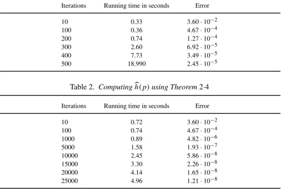
We can use Corollary 8·3 to computeh(p)without any factorisations, see Table 1. If we are only interested in a few digits of precision, it suffices to compute φn(p)forn 100. In this case the bulk of the computation is spent on the computation ofφn(p)forn 8, because, as mentioned in Section 9, we need to manipulate polynomials. For the computation ofφn(p)forn9 recurrence relations are used which only need the valuesφm(p)for a few
m <n, see Section 9.
If we are interested in more than 4 digits of precision, then the computation ofh(p)using Theorem 2·4 is much faster, see Table 2. The prime factorisation of the discriminant ofXis =28·86477, so it suffices to consider the set of placesS = {2,∞}, since phas integral
Table 1. Computingh(p)using Corollary8·3
Iterations Running time in seconds Error
10 0.33 3.60·10−2
100 0.36 4.67·10−4
200 0.74 1.27·10−4
300 2.60 6.92·10−5
400 7.73 3.49·10−5
500 18.990 2.45·10−5
Table 2. Computingh(p)using Theorem2·4
Iterations Running time in seconds Error
10 0.72 3.60·10−2
100 0.74 4.67·10−4
1000 0.89 4.82·10−6
5000 1.58 1.93·10−7
10000 2.45 5.86·10−8
15000 3.30 2.26·10−8
20000 4.14 1.65·10−8
25000 4.96 1.21·10−8
10·2. Order of growth ofλv(np)
As was remarked before, we are not able to say anything about the convergence rate of the sequence((1/n2)log|φ
n(p)|v)n∈T(p)for a given placevusing only Faltings’s Theorem 4·1. By (6·1), finding this convergence rate is equivalent to finding the order of growth ofλv(np). We have applied our implementation described in Section 9 to gather data on the asymp-totic behaviour and the implied constants of the sequence(λv(np))n∈N, where p ∈ J(Q) is a rational point on a genus 2 jacobian and v ∈ MQ. To this end we varied the place v, the coefficients μi and the point p. More precisely, we considered about 2000 random genus 2 curves with|μi| 50 fori ∈ {1, . . . ,4}; we computedλv(np)forv = ∞and all non-archimedeanvsuch that ordv()2, for all p^supp()J[2]of Kummer surface height bounded by 500 and for alln∈ {1, . . . ,15000}T(p). We also considered about 100 examples of curves with 50<|μi|1000.
10·2·1. Archimedean places
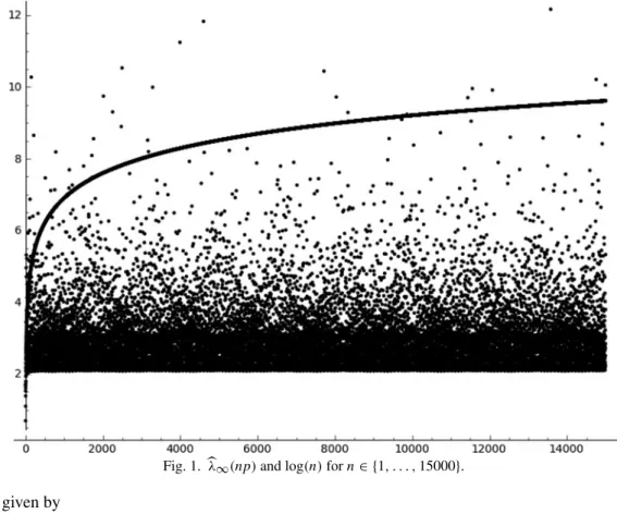
Let us first describe the casev= ∞. As mentioned in Remark 2, by a conjecture of Lang we should have
λ∞(np)=O(logn)
forn∈T(p). We have used our implementation to test this prediction.
See Figure 1 for the values ofλ∞(np), wheren ∈ {1, . . . ,15000}and p ∈ J1(Q)has
Mumford representation
(x2+1081/25x+148/5,13803/125x+1799/25).
Fig. 1.λ∞(np)and log(n)forn∈ {1, . . . ,15000}.
given by
y2=25+20x+30x2+40x3+50x4+x5.
All examples we have considered exhibit a similar behavior. The resulting data suggest that we may even have
λ∞(np)=O((logn)A)
for some 0 < A < 1 depending on X and p, and that the implied constant is rather small compared to the coefficientsμi.
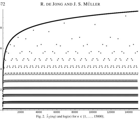
10·2·2. Non-archimedean places
LetJ2be the jacobian of the genus 2 curve given by
y2 =100+200x+300x2+400x3+500x4+x5
and letq ∈J2(Q)have Mumford representation
(x2+400x+200,3990x+1990).
Thenqreduces to a singular point on the reduction ofJ2modulov=2; the values ofλ2(nq)
are shown in Figure 2.
Note the apparent formation of finitely many horizontal lines, as well as a set of ‘sporadic’ points following the graph of logn. This dual behavior can perhaps be explained using Pro-position 3·1 (ii) and (iii) as follows: the set of specialisationsnp˜2of thenqin the special fiber
of the N´eron model modulovis a finite group R. The groupRhas a partitionR= R1R2
Fig. 2. λˆ2(nq)and log(n)forn∈ {1, . . . ,15000}.
λ2(nq)display a lognbehavior fornp˜2∈ R1, and are given byγ (C), withCthe component
containingnp˜2, whennp˜2∈ R2. Again, a similar behaviour occurred in all our examples.
Acknowledgements. We thank Yukihiro Uchida for providing us with formulas for the division polynomialsφn forn 5 wheng = 2. Some of the research described here was done while the second author was visiting the University of Leiden and he would like to thank the Mathematical Institute for its hospitality. The second author was supported by DFG grant KU 2359/2-1.
REFERENCES
[1] J. W. S. CASSELSand E. V. FLYNN.Prolegomena to a middlebrow arithmetic of curves of genus2. London Mathematical Society Lecture Note Series no. 230 (Cambridge University Press, 1996). [2] S. DAVIDand N. HIRATA–KOHNO. Linear forms in elliptic logarithms.J. Reine Angew. Math.628
(2009), 37–89.
[3] G. EVERESTand T. WARD. The canonical height of an algebraic point on an elliptic curve.New York J. Math.6(2000), 331–342.
[4] G. FALTINGS. Diophantine approximation on abelian varieties.Ann. of Math.(2)133(1991), 549– 576.
[5] E. V. FLYNNand N. P. SMART. Canonical heights on the Jacobians of curves of genus 2 and the infinite descent.Acta Arith.79(1997), 333–352.
[6] D. HOLMES. Computing N´eron–Tate heights of points on hyperelliptic Jacobians.J. Number Theory 132(2012), 1295–1305.
[7] N. KANAYAMA. Division polynomials and multiplication formulae of Jacobian varieties of dimension 2.Math. Proc. Camb. Phil. Soc.139(2005), 399–409.
[8] N. KANAYAMA. Corrections to “Division polynomials and multiplication formulae in dimension 2”. Math. Proc. Camb. Phil. Soc.149(2010), 189–192.
[9] S. LANG. Higher dimensional diophantine problems.Bull. Amer. Math. Soc.80(1974), 779–787. [10] S. LANG.Fundamentals of Diophantine Geometry(Springer–Verlag, 1983).
[11] MAGMA is described in W. BOSMA, J. CANNONand C. PLAYOUST. The Magma algebra system I: The user language.J. Symb. Comp.24(1997), 235–265.
[12] J. S. M ¨ULLER. Computing canonical heights using arithmetic intersection theory.Math. Comp.83
(2014), 311–336.
[13] J. S. M ¨ULLER. Explicit Kummer varieties of hyperelliptic Jacobian threefolds, to appear inLMS J. Comput. Math.(2014).
[14] J. S. M ¨ULLERand M. STOLL. Canonical heights on genus two Jacobians. In preparation. [15] M. STOLL. On the height constant for curves of genus two, II.Acta Arith.104(2002), 165–182. [16] M. STOLL. An explicit theory of heights for hyperelliptic Jacobians of genus three. In preparation. [17] Y. UCHIDA. Canonical local heights and multiplication formulas.Acta Arith.149(2011), 111–130. [18] Y. UCHIDA. Division polynomials and canonical local heights on hyperelliptic Jacobians.Manuscript.
Math.134(2011), 273–308.