Abstract ⎯In this paper, it is discussed notion of max-plus algebra and their properties. A model of flow shop production system and analyze the dynamical behavior of the system for scheduling problems are derived by means of max-plus algebra. The solutions of these problems are that the optimal sequence of jobs and the regular scheduling are obtained.
Keywords⎯Max - Plus Algebra, flow shop, scheduling.
I.INTRODUCTION
iscrete event systems can be used to study processes that are driven by occurrence of events. The relevant variables represent times at which events take place. In recent year both industry and the academic world have become interested to model, analyze and control complex systems such as manufacturing systems, traffic control system, and telecommunication network and so on. This kind of systems is typical examples of discrete event systems. One of the most characteristic features of a discrete event system is that its dynamics are event-driven in contrast with time driven. The behavior of a discrete event system is governed by events rather than by ticks of a clock. An event corresponds to the start or the end of an activity. If we consider of a production system then the possible events are the completion of a part on a machine, a buffer become empty, a machine breakdown and so on. Event occurs at discrete time instants. Interval between events are not necessarily identical, it can be deterministic or stochastic.
An introduction to Discrete Event Systems can be found in [3], and the application of traffic light system in [12]. Although in general discrete event systems lead to a non linear description in conventional algebra, there exists a subclass of discrete event systems for which this model becomes linear when we formulate it in the max-plus algebra notion. In this paper, we focus on of subclass of discrete event systems that is called max-plus algebra. This subclass can be used to analyze behavior of a system. The standard on the max-plus algebra approach to discrete event systems can be found in [1], and some results work of max-plus algebra in [2]. Some real application of max-plus algebra to transportation system can be found in [4, 8, 11], an assembly production process system in [7], and flow shop productionprocess
1Subiono is with the Department of Mathematics, Faculty of Mathematics and Natural Science, Institut Teknologi Sepuluh Nopember, Surabaya, 60111, Indonesia.
E-mail:[email protected]
2Nur Shofianah is Graduated Student of Master Program Mathematics Department, Faculty of Mathematics and Natural Science, Institut Teknologi Sepuluh Nopember, Surabaya, 60111, Indonesia.
with n job 2 machines in [10]. In this paper, we discuss flow shop production process and modify the model such that we get both a regular scheduling and a minimal makespan.
The model of the system by using max-plus algebra approach is derived; this approach will have an advantage. The system will be linear and non linear in conventional algebra [6]. The linearity makes the analysis on the behavior of system easy. Further in the following section, a brief introduction to max-plus algebra notion and notation is given. And as a motivation, we give an example application of max-plus algebra that is related to a periodic scheduling. This periodic scheduling associate is with an eigenvalue and an eigenvector of a square matrix in max-plus algebra. We use Max-Plus Algebra Toolbox for Scilab [9] to compute the eigenvalue and corresponding eigenvector of a square matrix in max-plus algebra. As conclusion, we give some notes of the discussion and the future work.
II.MAX-PLUS ALGEBRA AND SOME RELATED
NOTATION
This section presents a brief introduction to max plus algebra that would be employed in the following discussion. The element of max-plus algebra are real number and ε = -~. The set R ∪ {ε} will be denoted by Rmax with R is the set of real number. The basic
operations of Max-Plus Algebra are maximization
(denoted by symbol⊕) and addition (denoted by symbol⊗). With these two operations for allx,y∈Rmax,
we get: { }x,y max y
x⊕ = and x⊗y=x+y and, in the context of
Max-Plus Algebra
max b: ab, a R
a⊗ = ∈ and b∈R
So, we get 3⊗4=4(3)=12 and
6 ) 12 ( 2 1 12 2
1
− = − =
−
⊗ .
Note that: for every x∈Rmax that satisfies x⊕ε=x=ε⊕x
andx⊗0=x=0⊗x.
As in the conventional algebra, it is well known that a matrix with real number entries and two operations addition and multiplication. In the max-plus algebra Rmax, two operations addition and multiplication are
denoted by two symbols respectively ⊕ and⊗. For two matrices over Rmax, the addition of matricesA,B Rmmaxn
×
∈ , be
given by:
[A B]i ,j ai,j bi,j max
{
ai,j,bi,j}
⊕ = ⊕ = with i = 1,2,…,m and j =
1,2,…,n. And multiplication of two matrices mp max R A∈ × and
n p max R
B∈ × be given by [ ]
{
}
, max
, , 1kp , ,
1
, ik kj ik kj p
k j
i a b a b
B
A⊗ =⊕ ⊗ = +
≤ ≤ =
with
i = 1,2,…,m and j = 1,2,…,n.
Using Max-Plus Algebra in The Flow Shop
Scheduling
Subiono1 and Nur Shofianah21
It is shown that there is an analogy between ⊕ and
+
and, ⊗ and ×. Therefore we choose the symbols ⊕and ⊗. And multiplication of two matrices in max-plus algebra is similar to multiplication of two matrices in conventional algebra, i.e. two operations multiplication and addition in the conventional algebra and "maximization (⊕)" and "addition (⊗)" in the max-plus algebra as replacement of respectively addition and multiplication that are used in the conventional algebra. With these symbols, the description of state space of a system be given by equations as follow:
) k ( x C ) k ( y
) 1 k ( u B ) k ( x A ) 1 k ( x
⊗ =
+ ⊗ ⊕ ⊗ =
+ (1)
with the size of the matrices in equation (1) satisfies addition and multiplication of matrices.
Like conventional algebra, an eigenvalue and a corresponding eigenvector of a square matrix A of size n x n also exists in max-plus algebra, i.e. if we give the equation
x x A⊗ =λ⊗ .
In this case vector x Rn max
∈ and scalar λ∈R are
respectively called an eigenvector and a corresponding
eigenvalue of the matrix A with vectorx≠
(
ε,L,ε)
' . The sign ′ represents transpose. An algorithm to compute an eigenvalue and a corresponding eigenvector of a square matrix A can be found in [5].Example 1: Let be a matrix
, 5
3 4
2 1
⎟ ⎟ ⎟
⎠ ⎞
⎜ ⎜ ⎜
⎝ ⎛ =
ε ε
ε ε
A it follows that,
⎟ ⎟ ⎟
⎠ ⎞
⎜ ⎜ ⎜
⎝ ⎛ ⊗ = ⎟ ⎟ ⎟
⎠ ⎞
⎜ ⎜ ⎜
⎝ ⎛ = ⎟ ⎟ ⎟
⎠ ⎞
⎜ ⎜ ⎜
⎝ ⎛ ⊗ ⎟ ⎟ ⎟
⎠ ⎞
⎜ ⎜ ⎜
⎝ ⎛
3 2 0 4 7 6 4
3 2 0
5 3 4
2 1
ε ε
ε ε
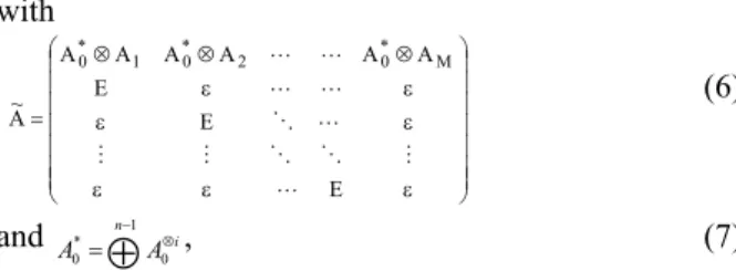
It is shown that the eigenvalue and corresponding eigenvector of matrix A are respectively λ = 4 and x = (0 2 3)T. Let be given matrix nn
max R
A∈ × , a directed graph of
matrix A is denoted by G(A) = (E,V). Graph G(A) has n
nodes (vertices), the set of all nodes of graph G(A) is denoted by V. An arc (edge) from node j to i occurs if ai,j
≠ε, this arc is denoted by (j,i). The set of all arcs of graph G(A) is denoted by E. The weight of arc (j,i) is value of ai,j, this one is denoted by w(j,i) = ai,j. If ai,j = ε, then arc
(j,i) does not exist. A sequence of arc (i1,i2), (i2,i3),…, (i l-1,il) of a graph is called a path. A path is called elementer
if it nodes has only one incoming and one outgoing arc. A circuit is a close elementer path, i.e.:
(i1,i2), (i2,i3),…, (il-1,il). The weight of a path p = (i1,i2),
(i2,i3),…, (il-1,il) is denoted by |p|w with
(
i2,i1 i3,i2 il,il1)
w a a a
| p
| = + +L+ − .
The length of a path p is the sum of arc in the path p and it is denoted by |p|l. The average weight of a path p is
the weight of path p divided by the length of path p, i.e.
(
)
1 l
a a
a | p |
| p
| i2i,1 i3i,2 ili,l1
l w
− + + +
= L −
.
Circuit mean is the average weight of a circuit. Any circuit with maximum circuit mean is called critical circuit. A graph is called strongly connected graph if a path exists for every node i to every node j. If graph G(A) is strongly connected, then the matrix A is called
irreducible.
Fig. 1 is graph G(A) of Example 1. There are three circuits, i.e. (1,1); (1,2),(2,1) and (2,3),(3,2). Each circuit
has circuit mean: 4
2 3 5 ; 3 2
2 4 ; 1 1
1= + = + = . It is shown that
the maximum circuit mean equals 4. This circuit is (2,3),(3,2) and this one is the critical circuit of grap G(A).
The graph G(A) is strongly connected. Some notion that have discussed have been implemented in the toolbox [9]. The interpretation of the eigenvalue and the corresponding eigenvector of Example 1 as follows: Let be given three activities (nodes of graph G(A)), that ones periodically operated. Each node has its own kind of activity. It is assumed that an activity at certain node can only start when all preceding nodes have finished their activities and send the results of these activities along the arcs to the current node. Thus, the arc corresponding to ai,j can be interpreted as an output for node j and
simultaneously as input for node i. Suppose that this node i starts its activity as soon as all preceding nodes have sent their results to node i. So an activity only can starts its activity at (k+1)-th time if all preceding activities have finished their activities and sent their results at k-th time. Element ai,j of matrix A represents
the sum of the activity time of node j and the travelling time from node j to node i. If element ai,j = ε, then the
activity i does not depend on the activity j. If xi (k) is the
earliest epoch at which node i become active for the k-th time with i =1, 2, 3, then the evolution of the system of Example 1 is given by difference equation of 1st-orde x (k+1) = A⊗ x(k), k = 0, 1, 2, … (2)
If it is chosen x(0) as the eigenvector of matrix A, then system (2) will operate as periodic with periodicity equals the eigenvalue λ=4. This follows the equation: x(k+1) = A ⊗x(k)
= λ⊗(k+1)⊗x(0), k = 0, 1, 2, … (3)
and we get the regular activities sequence x(k):
L
⎟ ⎟ ⎟
⎠ ⎞
⎜ ⎜ ⎜
⎝ ⎛
⎟ ⎟ ⎟
⎠ ⎞
⎜ ⎜ ⎜
⎝ ⎛
⎟ ⎟ ⎟
⎠ ⎞
⎜ ⎜ ⎜
⎝ ⎛
⎟ ⎟ ⎟
⎠ ⎞
⎜ ⎜ ⎜
⎝ ⎛
⎟ ⎟ ⎟
⎠ ⎞
⎜ ⎜ ⎜
⎝ ⎛
⎟ ⎟ ⎟
⎠ ⎞
⎜ ⎜ ⎜
⎝ ⎛
⎟ ⎟ ⎟
⎠ ⎞
⎜ ⎜ ⎜
⎝ ⎛
27 26 24 , 23 22 20 , 19 18 16 , 15 14 12 , 11 10 8 , 7 6 4 , 3 2 0
For nonnegative number M > 0, let be a matrix
nxn
m R
A ∈ max for 0 < m < M and x(m)∈Rmaxn for -M < m < -1,
then the difference equation of Mth-order will be written as follows: x(k) A x(k m), k 0.
0 ⊗ − ≥
⊕ =
= m M
m
(4)
The Equation (2) is a difference equation of 1st-orde and A0 = ε. A difference equation of Mth-orde with A0≠
ε can be transformed into a difference equation of 1st-order that is given by Equation (2), as follows
0, k ), k ( X ~ A~ ) 1 k (
X~ + = ⊗ ≥ (5)
with
⎟⎟ ⎟ ⎟ ⎟ ⎟ ⎟
⎠ ⎞
⎜⎜ ⎜ ⎜ ⎜ ⎜ ⎜
⎝ ⎛
ε ε
ε
ε ε
ε ε
⊗ ⊗
⊗
=
E
E
E
A A A A A A
A~
M * 0 2
* 0 1 * 0
L
M O O M M
L O
L L
L L
(6)
and n i i
A A − ⊗
=
⊕
= 0
1
0 *
0 , (7)
Matrix E is identity matrix. This can be found in [2].
III.SCHEDULING OF FELLOW SHOP
thoroughly. Such a model is given a flow shop production of n job {Ji} that will be scheduled on m
machines {Mk} with 1< i < n and k = 1, 2. Each job must
be processed exactly at a time in each machine by means of the same machine ordering. Permutation flow shop is a special class of flow shop by which each job would have the same processing order in each machine. Assuming is no set-up time between job operations. A dynamical model of flow shop production is constructed in [10] and an example is given. It is shown that the model has a regular scheduling. But it is not an optimal scheduling due to the makespan that is greater than the minimal one. Therefore, in this paper, the model is modified in such a way that it has a regular scheduling and minimal makespan. Firstly, it begins with analyzing some important factors of the model to decide when starting job processing of each cyclic production. Then, the analyses of flow job as a cycle of (periodic) production and, a job notion will be replaced by an operation to make clearer job ordering. Thus, giving a flow shop of 2 job, 2 machines, job J1 in machine M1 and
J1 in M2 respectively will be called first and second
operation. Therefore, the ordering of the same job J1
processed in the different machine M1 and M2 more
clearly. If xij (k+1) represents starting time of j-th
operation in i-th machine for (k+1)-th period and pij
represents time processing of j-th operation in i-th machine, then xij (k+1) will be a maximization of :
Release time of i-th machine for k-th period, i.e. completion operations for k-th period in i-th machine, this will be denoted by yi(k), and yi(0) for k = 0.
It is assumed that initial time of resources in each job is ready for first period so rij(0) = 0 for k = 0. There are
no preceding jobs for the first job, so we define
i k i ij k r =⊗λ
=1 )
( for k = 1, 2, … For the first operation of
second job and the next job, the initial time of ready resources is the sum of period time and processing time of all preceding jobs operation, i.e.
mn M mP n i k i
ijk p
r j ⊗ ⊗ = ∈ ∈ =1λ ) (
with λi = λ represents period time (the eigenvalue of
transition matrix of the model before modified [10]) ; the set of all preceding j operation is denoted by Pj and
M represents a machine. Therefore Pmn represents
processing time of operation n in machine m with preceding process n is processing j in machine i.
The completion time of all preceding operation of j
operation, includes:
Processed operations in each machine of (k+1)-th period. If Pj is set of all preceding j operation of corresponding
job, then for n∈ Pj and m ∈ M, completion time of all
preceding j operation of (k+1)-th period is given by
xmn(k+1) + pmn. If j operation is the first operation of an
job, then this one has no preceding operation.
Other scheduled operation (l≠j and l∈P) that early processing of j operation in i machine of (k+1)-th period is represented in xil (k+1) + pil
.
So we can write xil (k+1) as
xij(k+1)= max{yi(k),rij(k),pmn(k+1)+xmn(k+1),pil+xil(k+1)
or in the Max-Plus Algebra as
) 1 ( ) 1 ( ) 1 ( ) ( ) ( ) 1 ( + ⊗ ⊕ + ⊗ + ⊕ ⊕ = + k x p k x k p k r k y k x il il mn mn ij i
ij (8)
Release time in each 1-machine and 2-machine represented } ) ( , , ) ( , ) ( max{ ) ( ) 1 ( 1 ) 1 ( 1 13 13 11 11 1 − − + + + = n
n k p
x p k x p k x k y L L } ) ( , , ) ( , ) ( max{ ) ( 1 2 34 4 , 2 22 22 2 n nk p
x p k x p k x k y + + + = L L
or in the Max-Plus Algebra as
⎪ ⎪ ⎩ ⎪⎪ ⎨ ⎧ ⊗ ⊕ ⊕ ⊗ ⊕ ⊗ = ⊗ ⊕ ⊕ ⊗ ⊕ ⊗ = − − n n n n p k x p x p x y p k x p x p x y 2 2 24 24 22 22 2 ) 1 ( 1 ) 1 ( 1 13 13 11 11 1 ) ( ) ( L L L L (9)
and from Equation (8) and (9) the modified model can be written as follows:
) 1 ( ) 1 ( ) 1 ( ) ( ) ( ) 1 ( 2 0 + ⊗ = + + ⊗ ⊕ ⊕ = + k X A k Y k X A k R k Y k X (10) With ⎟⎟ ⎠ ⎞ ⎜⎜ ⎝ ⎛ = ⎟⎟ ⎠ ⎞ ⎜⎜ ⎝ ⎛ = 0 0 ) 0 ( y ) 0 ( y ) 0 ( y 2 1 and ⎪⎩ ⎪ ⎨ ⎧ = ⊗ = = =
⊗
∈= for 1,2,L
0 for 0 ) ( ) ( , ,
1 p k
k k
r k
R mn
P n m i k i ij j λ
Equation (10) can be rewritten as difference equation of 1st-order as follows:
) ( ) ( ) 1 ( ) 1
(k A0 X k A1 X k Rk
X + = ⊗ + ⊕ ⊗ ⊕ (11)
The solution can be found by transforming Equation (11) into difference equation 1st-order as Equation (5), i.e. : ) ( ) ( ~ ~ ) 1 ( ~ k R k X A k
X + = ⊗ ⊕ (12)
with 0* 1 ~
A A
A= ⊗ and n i i
A A − ⊗
=
⊕
= 0 1 0 * 0Example 2 Let be given flow shop production system that contains two jobs J1 and J2 scheduled in two
machines M1 and M2 with time processing is given by
Table 1.
By using Equation (11) and transforming this one into Equation (12), we get the modified model as follows:
⊕ ⎟⎟ ⎟ ⎟ ⎟ ⎠ ⎞ ⎜⎜ ⎜ ⎜ ⎜ ⎝ ⎛ ⊗ ⎟⎟ ⎟ ⎟ ⎟ ⎠ ⎞ ⎜⎜ ⎜ ⎜ ⎜ ⎝ ⎛ = ⎟⎟ ⎟ ⎟ ⎟ ⎠ ⎞ ⎜⎜ ⎜ ⎜ ⎜ ⎝ ⎛ + + + + ) ( ) ( ) ( ) ( 6 5 6 5 3 2 3 2 ) 1 ( ) 1 ( ) 1 ( ) 1 ( 24 22 13 11 24 22 13 11 1 k x k x k x k x k x k x k x k x
A4 34
4 4 2 1ε ε
ε ε ε ε ε ε 43 42 1 4 4 3 4 4 2 1 ) ( 13 11 24 22 13 11 ) ( ) ( ) 1 ( ) 1 ( ) 1 ( ) 1 ( 5 3 2 2
0 Rk
A k r k r k x k x k x k x ⎟⎟ ⎟ ⎟ ⎟ ⎠ ⎞ ⎜⎜ ⎜ ⎜ ⎜ ⎝ ⎛ ⊕ ⎟⎟ ⎟ ⎟ ⎟ ⎠ ⎞ ⎜⎜ ⎜ ⎜ ⎜ ⎝ ⎛ + + + + ⊗ ⎟⎟ ⎟ ⎟ ⎟ ⎠ ⎞ ⎜⎜ ⎜ ⎜ ⎜ ⎝ ⎛ ε ε ε ε ε ε ε ε ε ε ε ε ε ε ) ( ) ( ) 1 ( ) 1
(k A0 X k A1 X k Rk
X + = ⊗ + ⊕ ⊗ ⊕
And it is transformed as ) ( ) ( ~ ~ ) 1 ( ~ k R k X A k
X + = ⊗ ⊕
So, we get
,
29 24 24 22
,
18 13 13 11
,
7 2 2 0
x(3) x(2) x(1)
⎟⎟ ⎟ ⎟ ⎟
⎠ ⎞
⎜⎜ ⎜ ⎜ ⎜
⎝ ⎛
⎟⎟ ⎟ ⎟ ⎟
⎠ ⎞
⎜⎜ ⎜ ⎜ ⎜
⎝ ⎛
⎟⎟ ⎟ ⎟ ⎟
⎠ ⎞
⎜⎜ ⎜ ⎜ ⎜
⎝ ⎛
(13)
or one can be rewritten in the following form
⎟⎟ ⎟ ⎟ ⎟
⎠ ⎞
⎜⎜ ⎜ ⎜ ⎜
⎝ ⎛
⊗ ⊗ = ⎟⎟ ⎟ ⎟ ⎟
⎠ ⎞
⎜⎜ ⎜ ⎜ ⎜
⎝ ⎛
⊗ ⊗ ⊗ ⊗
= +
0 0 0 0
) 1 (
) 1 (
) 1 (
) 1 (
) 1 (
) 1 (
24 13 22 11
λ
λ λ λ λ
k x
k x
k x
k x
k x
k
x (14)
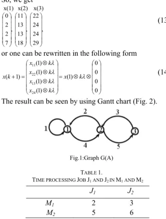
The result can be seen by using Gantt chart (Fig. 2).
Fig.1:Graph G(A)
TABLE 1.
TIME PROCESSING JOB J1 AND J2IN M1 AND M2 J1 J2
M1 2 3
M2 5 6
If the initial time of ready resources at 07.00 is written as 00 in the Table 2 and unit time processing in minute, then from scheduling of Equation (12) it can identify processing J1 in M1 (denoted by node x1)
starting at 07.00. Processing job J2 in M1 (x2) and J1 in
M2 (x3) at 07.02 is written as 02. And processing J2 in M2
(x4) at 07.07 is written as 07. In the same way, by using
07.00 as a reference time, we can know starting time of the next period processing that is given by Table 2.
From Fig. 2, it is shown that the system periodic with period equals 11 unit time and makespan 13 unit time, this result exactly equal to makespan as it is calculated in [13], i.e. firstly we make job matrix as follow:
⎟⎟ ⎠ ⎞ ⎜⎜
⎝ ⎛ =
2 ,
2 , 1 , 1 , ) (
x x x x
x p
p p p J
M ε
with M(J[i]) represents job matrix and p[i],k is time
processing, 1 < i < n and k = 1, 2, … So we get
⎟⎟ ⎠ ⎞ ⎜⎜ ⎝ ⎛ = ⎟⎟ ⎠ ⎞ ⎜⎜ ⎝
⎛ ⊗
=
5 7 2 5
5 2 2 )
(J1 ε ε
M
⎟⎟ ⎠ ⎞ ⎜⎜ ⎝ ⎛ = ⎟⎟ ⎠ ⎞ ⎜⎜ ⎝
⎛ ⊗
=
6 9 3 6
6 3 3 )
(J2 ε ε
M
⎟⎟ ⎠ ⎞ ⎜⎜
⎝ ⎛
⊗ ε
⊗ ⊕ ⊗ ⊗
=
⊗ = σ =
σ = σ
⊗ ⊗
= σ
=
) 2 ( p ) 1 ( p
) 2 ( p ) 1 ( p ) 2 ( p ) 1 ( p ) 2 ( p ) 1 ( p
) J ( M ) J ( M )) i ( ( M
)) i ( ( M ) ( M
2 2
2 2 , 1 2 , 1 1 1 1
2 1 2
1 i
| |
1 i
⎟⎟ ⎠ ⎞ ⎜⎜ ⎝ ⎛ =
⎟⎟ ⎠ ⎞ ⎜⎜
⎝ ⎛
⊗ ⊗ ⊕ ⊗ ⊗ =
11 13 5
6 5
) 6 7 ( ) 9 2 ( 3 2
ε
ε
Therefore, makespan can be calculated from equation in below:
( )
( ) (5 13)
11 13 5 0
) ( 0 ) (
= ⎟⎟ ⎠ ⎞ ⎜⎜ ⎝ ⎛ ⊗ =
⊗ =
ε ε
σ ε
σ M
C
It is shown that completion time in M1 equals 5 and
completion time in M2 equals 13. So, makespan of this
case equals 13. With the same ordering job, this makespan less than initial makespan of Example in [10] that equals 17.
Therefore, Equation (12) can be used to obtain regular production model with minimum makespan and scheduling of starting process can be obtained by using Equation (14).
Fig. 2. Gantt chart production flow of flow shop 2 jobs 2 machines of Example 2 ( modified model)
TABLE 2
SCHEDULING OF STARTING PROCESS OF EXAMPLE 2FOR3 CYCLES PRODUCTION
1 2 3
J1 J2 J1 J2 J1 J2
M1 0 2 11 13 22 24
M2 2 7 13 18 24 29
IV.CONCLUSION
In this section describe some notes for discussing especially flow shop scheduling. The modified model given by:
) 1 ( )
1 (
) 1 ( )
( ) ( ) 1 (
2
0
+ ⊗ = +
+ ⊗ ⊕ ⊕ = +
k X A k Y
k X A k R k Y k X
with ⎟⎟
⎠ ⎞ ⎜⎜ ⎝ ⎛ = ⎟⎟ ⎠ ⎞ ⎜⎜ ⎝ ⎛ =
0 0 ) 0 ( y
) 0 ( y ) 0 ( y
2 1
and
⎪⎩ ⎪ ⎨ ⎧
= ⊗
= =
=
⊗
∈
= for 1,2,L 0 for 0 ) ( )
( ,
,
1 p k
k k
r k
R mn
P n m i k
i ij
j
λ
This model can be rewritten as a difference equation of 1st-order with A0 ≠ ε:
) ( ) ( )
1 ( )
1
(k A0 X k A1 X k Rk
X + = ⊗ + ⊕ ⊗ ⊕ .
Next, we transform the model and get a new model that is given by:
) ( ) ( ~ ~ ) 1 (
~ k A X k Rk
X + = ⊗ ⊕ with 1
* 0
~ A A
A= ⊗ and n i i
A A − ⊗
=
⊕
= 0
1 0 * 0
The scheduling of this model is regular and it has the minimal makespan. This result gives an idea to make model of flow shop production by using max-plus algebra. For the future work, the discussing can be continued for flow shop production with set-up time and more than two machines. The case of more than two machines the problem is NP-Hard [14].
REFERENCES
[1] F. Baccelli, G. Cohen, G.J. olsder, and J.-P. Quadrat, 1992, Synchronization and linearity: Analgebra for Discrete Event Systems, Wiley.
[3] C. Cassandras and S. Lafortune, 1999, Introduction to Discrete Event Systems, Kluwer Academic Publisher.
[4] Subiono, 2000, On Classes of Min-max-plus Systems and Their Application, PhD Thesis, Delft University of Technology, the Netherlands.
[5] Subiono and J. van der Woude, 2000, Power Algorithms for
(max,+)-and Bipartite (min,max,+)-Systems, Discrete Event Dynamic Systems:Theory and Applications, 10(4):369-389. [6] Subiono, 2000, Operator Linier dalam Aljabar Max Plus dan