arXiv:0907.2676v3 [math.DS] 29 Jan 2010
ASSOCIATED WITH PISOT UNITS
CHARLENE KALLE AND WOLFGANG STEINER
Abstract. From the works of Rauzy and Thurston, we know how to construct (multiple) tilings of some Euclidean space using the conjugates of a Pisot unitβand the greedyβ-transformation. In this paper, we consider different transformations generating expansions in baseβ, including cases where the associated subshift is not sofic. Under certain mild conditions, we show that they give multiple tilings. We also give a necessary and sufficient condition for the tiling prop-erty, generalizing the weak finiteness property (W) for greedyβ-expansions. Remarkably, the symmetricβ-transformation does not satisfy this condition whenβis the smallest Pisot number or the Tribonacci number. This means that the Pisot conjecture on tilings cannot be extended to the symmetricβ-transformation.
Closely related to these (multiple) tilings are natural extensions of the transformations, which have many nice properties: they are invariant under the Lebesgue measure; under certain con-ditions, they provide Markov partitions of the torus; they characterize the numbers with purely periodic expansion, and they allow determining any digit in an expansion without knowing the other digits.
1. Introduction
Tilings generated by substitutions and theβ-transformation are well-studied objects from var-ious points of view. Tilings from substitutions were first introduced by Rauzy in the seminal paper [Rau82]. For the β-transformation, Tβx = βxmod 1, β > 1, Thurston laid the ground
work in [Thu89]. The transformation Tβ can be used to obtain the greedyβ-expansion of every
x∈[0,1) by iteration. The expansions obtained in this way are expressions of the form
(1) x=
∞ X
k=1
bk
βk,
where the digits bk are all elements of the set {0,1, . . . ,⌈β⌉ −1}. Here,⌈x⌉denotes the smallest
integer larger than or equal tox. The expansions that Tβ produces are greedy in the sense that,
for eachn ≥1,bn is the largest element of the set {0,1, . . . ,⌈β⌉ −1} such that Pnk=1bkβ−k ≤
x. Thurston defined tiles in Rd−1 when β is a Pisot unit of degree d. Akiyama ([Aki99]) and Praggastis ([Pra99]), independently of one another, showed that these tiles form a tiling ofRd−1 when β satisfies the finiteness property (F) defined in [FS92] by Frougny and Solomyak, which means that the set of numbers with finite greedy expansion is exactlyZ[β−1]
∩[0,1). They also showed that the origin is an inner point of the central tile in this case.
The tiles can be constructed by using two-sided admissible sequences. These are sequences · · ·w−1w0w1w2· · · of elements from the digit set {0,1, . . . ,⌈β⌉ −1} such that each right-sided
truncation wkwk+1· · · corresponds to an expansion generated by Tβ. In some sense, this
con-struction makes the non-invertible transformation Tβ invertible at the level of sequences. In
ergodic theory, a way to replace a non-invertible transformation by an invertible one, without losing its dynamics, is by constructing a version of the natural extension. A natural extension of a non-invertible dynamical system is an invertible dynamical system that contains the original dynamics as a subsystem and that is minimal in a measure theoretical sense. Much theory about natural extensions was developed by Rohlin ([Roh61]). He gave a canonical way to construct a
Date: January 29, 2010.
2000Mathematics Subject Classification. 11A63, 11R06, 28A80, 28D05, 37B10, 52C22, 52C23.
natural extension and showed that the natural extension is unique up to isomorphism. Many properties of the original dynamical system can be obtained through the natural extension, for example all mixing properties of the natural extension are inherited by the original system. The tilings described above and natural extensions ofTβ are thus closely related concepts.
The question of whether or not Thurston’s construction gives a tiling when conditions are re-laxed, is equivalent to a number of questions in different fields in mathematics and computer sci-ence, like spectral theory (see Siegel [Sie04]), the theory of quasicrystals (Arnoux et al. [ABEI01]), discrete geometry (Ito and Rao [IR06]) and automata ([Sie04]). In [Aki02], Akiyama defined a weak finiteness property (W) and proved that it is equivalent to the tiling property. He also stated there that it is likely that all Pisot units satisfy this condition (W). It is thus conjectured that we get a tiling of the appropriate Euclidean space for all Pisot unitsβ. This is a version of the Pisot conjecture, which is discussed at length in the survey paper [BS05] by Berth´e and Siegel. Classes of Pisot numbersβ satisfying (W) are given in [FS92, Hol96, ARS04, BBK06].
The transformation Tβ is not the only transformation that can be used to generate number
expansions of the form (1) dynamically. In [EJK90], Erd˝os et al. defined the lazy algorithm that also gives expansions with digits in the set{0,1, . . . ,⌈β⌉ −1}. In [DK02], Dajani and Kraaikamp gave a transformation, which they called the lazy transformation, that generates exactly these expansions in a dynamical way. This transformation is defined on the extended interval0,⌈ββ⌉−−11. Pedicini ([Ped05]) introduced an algorithm that produces number expansions of the form (1), but with digits in an arbitrary finite set of real numbers A. He showed that if the difference between two consecutive elements inA is not too big, then every xin a certain interval has an expansion with digits in A. These expansions generalize the greedy expansions with digits in {0,1, . . . ,⌈β⌉ −1}, and are thus called greedy β-expansions with arbitrary digits. In [DK08], a lazy algorithm is given by Dajani and the first author, that can be used to get lazy expansions with arbitrary digits. In the same article, both a greedy and lazy transformation are defined to generate expansions with arbitrary digits dynamically. Another type of transformations that generate expansions like (1), but with digits in{−1,0,1}, is given in [FS08] by Frougny and the second author. It is shown there, among other things, that for specific β > 1 and α > 0, the transformationT : [−βα, βα)→[−βα, βα) defined byT x=βx− ⌊ x
2α+ 1
2⌋providesβ-expansions
of minimal weight, i.e., expansions in which the number of non-zero digits is as small as possible. These expansions are interesting e.g. for applications to cryptography.
In this paper, we consider a class of piecewise linear transformations with constant slope, that contains all the transformations mentioned above. By putting some restrictions onβ and on the digit set, we can mimic the construction of a tiling of a Euclidean space, as it is given in [Aki02]. We establish some properties of the tiles we obtain by this construction and state conditions under which these tiles give a multiple tiling.
tilings where the underlying shift space is non-sofic and which are not self-affine in the sense of [Pra99] and [Sol97]. In some examples, some tiles consist of a single point or of countably many points and have therefore zero Lebesgue measure.
Remarkable examples of double tilings come from the symmetricβ-transformation defined by Akiyama and Scheicher ([AS07]), for two Pisot unitsβ: the Tribonacci number and the smallest Pisot number. This means that the Pisot conjecture cannot be extended to the symmetric β -transformation. It is unclear why the Tribonacci number and the smallest Pisot number give double tilings while many other Pisot units give tilings, and it is possible that getting more insight into this question may lead to a proof or a disproof of the Pisot conjecture.
2. Admissible sequences
Throughout the paper, we consider transformationsT : X →X defined by T x=βx−a for x∈ Xa, a∈ A, where A is a finite subset of R, X is the disjoint union of non-empty bounded
setsXa ⊂R, andβ >1. We are interested in the digital expansions generated byT, as defined in
Definition 2.1. We denote byAω the set of right infinite sequences with elements inA, and by
the lexicographical order onAω.
Definition 2.1 (T-expansion,T-admissible sequence). LetT be as in the preceding paragraph. Forx∈X, the sequenceb(x) =b1(x)b2(x)· · · ∈Aωsatisfyingbk(x) =aifTk−1(x)∈Xa,a∈A, is
called theT-expansionofx. A sequenceu∈Aωis calledT-admissible ifu=b(x) for somex
∈X. Note thatT x=βx−b1(x), sox= (b1(x) +T x)/β, and inductively
(2) x=
n
X
k=1
bk(x)
βk +
Tnx
βn
for alln≥1. SinceX is bounded, we have limn→∞(Tnx)β−n = 0 and thusx=P∞k=1bk(x)β−k.
Therefore, we define thevalue of a sequenceu=u1u2· · · ∈Aω by.u=Pk≥1ukβ−k.
A first characterization ofT-admissible sequences is given by the following lemma.
Lemma 2.2. A sequenceu=u1u2· · · ∈Aω isT-admissible if and only if .ukuk+1· · · ∈Xuk for allk≥1.
Proof. For eachk≥1, set xk =.ukuk+1· · ·. Suppose first that u=b(x) for somex∈X. Then
we havex=.b(x) =.u=x1, hence xk =Tk−1x∈Xuk for allk≥1. Now suppose that xk ∈Xuk
for allk≥1. ThenT xk =βxk−uk=xk+1 for eachk≥1, henceu=b(x1).
Theorem 2.5 provides a simpler characterization, whenT satisfies some additional conditions.
Lemma 2.3. Let x, y∈X and assume that supXa ≤infXa′ for all a < a′. Then we have x < y if and only if b(x)≺b(y).
Proof. Clearly, b(x) = b(y) is equivalent to x = y. So we can assume that there exists some k≥1 such thatb1(x)· · ·bk−1(x) =b1(y)· · ·bk−1(y) andbk(x)6=bk(y). Then x < yis equivalent
to Tk−1x < Tk−1y by (2). Since we have Tk−1x
∈ Xbk(x), T k−1y
∈ Xbk(y), we obtain that
Tk−1x < Tk−1y,b
k(x)6=bk(y), is equivalent tobk(x)< bk(y). This proves the lemma.
From now on, we assume that the sets Xa are finite unions of left-closed, right-open intervals
and thatT X =X, i.e., thatSa∈AT Xa=Sa∈A(βXa−a) =X.
Definition 2.4 (Left-, right-continuousβ-transformation). Let β > 1, let A be a finite subset of R, X be the disjoint union of non-empty sets Xa, a∈ A, where each Xa is a finite union of
intervals [ℓi, ri)⊂R,i∈Ia, andSa∈A(βXa−a) =X. Then we call the mapT : X →X defined
byT x=βx−afor allx∈Xa,a∈A, aright-continuousβ-transformation.
The correspondingleft-continuousβ-transformation Te: Xe →Xe is defined byT xe =βx−afor x∈Xea, whereXea =Si∈Ia(ℓi, ri] for eacha∈Aand Xe=Sa∈AXea. Forx∈Xe, theTe-expansion
ofxis denoted by ˜b(x).
Theorem 2.5. LetTbe a right-continuousβ-transformation, where eachXa,a∈A, is a single in-terval[ℓa, ra), andra ≤ℓa′ ifa < a′. LetTebe the corresponding left-continuousβ-transformation.
Then a sequence u=u1u2· · · ∈Aω isT-admissible if and only if
(3) b(ℓuk)ukuk+1· · · ≺˜b(ruk) for allk≥1.
A sequenceu=u1u2· · · ∈Aω isTe-admissible if and only if
b(ℓuk)≺ukuk+1· · · ˜b(ruk) for allk≥1.
Proof. We will prove only the first statement, since the proof of the second one is very similar. If u = b(x) for some x ∈ X, then Tk−1x
∈ Xuk = [ℓuk, ruk) and b(T
k−1x) = u
kuk+1· · ·
for all k ≥ 1. By Lemma 2.3, we obtain immediately that b(ℓuk) b(T
k−1x). We show that
b(Tk−1x)
≺˜b(ruk). SinceTk−1x < ruk, there must be an indexnsuch thatbn(Tk−1x)6= ˜bn(ruk)
andbi(Tk−1x) = ˜bi(ruk) for alli < n. Thus,Tn+k−2x <Ten−1ruk, which implies thatbn(Tk−1x)<
˜bn(ruk). Hence, b(Tk−1x)
≺˜b(ruk) and (3) holds.
For the other implication, suppose thatu satisfies (3) and setxk =.ukuk+1· · · for all k≥1.
By Lemma 2.2, it suffices to show that xk ∈ [ℓuk, ruk) for all k ≥ 1. Since uk = ˜b1(ruk), there
exists somes(k)> k such thatuk· · ·us(k)−1= ˜b1(ruk)· · ·˜bs(k)−k(ruk) andus(k)<˜bs(k)−k+1(ruk).
Then we have
ruk−xk=
e
Ts(k)−kr
uk−xs(k)
βs(k)−k >
ℓ˜bs(k)
−k+1(ruk)−xs(k)
βs(k)−k ≥
rus(k)−xs(k)
βs(k)−k
for allk≥1. By iteratingsn(k) =s(sn−1(k))> sn−1(k),n≥1, we obtain
ruk−xk > lim n→∞
rusn(k)−xsn(k)
βsn(k)−k = 0,
where we have used that{xk : k≥1}is bounded and that limn→∞sn(k) =∞. Similarly, we can show thatxk≥ℓuk for allk≥1, hence the theorem is proved.
Remark 2.6. With the assumptions of Theorem 2.5, we haveb1(ℓuk) = ˜b1(ruk) =uk for allk≥1.
If T ℓuk = minX, then the condition b(ℓuk)ukuk+1· · · follows from b(ℓuk+1) uk+1uk+2· · ·.
Similarly,T re uk= maxXe implies thatukuk+1· · · ≺˜b(ruk) follows fromuk+1uk+2· · · ≺˜b(ruk+1).
Remark 2.7. In all our examples, the conditions of Theorem 2.5 are fulfilled and X is a half-open interval, the sets Xa are thus consecutive half-open intervals. However, the more general
Definition 2.4 is needed at several points in this paper, e.g. in the proof of Proposition 4.6, for the transformationTY in Section 4.5.2 and when we restrictT to the support of its invariant measure. Example 2.8. Consider the classical greedy β-transformation, Tβx= βxmod 1. This fits in the
above framework if we takeA = {0,1, . . . ,⌈β⌉ −1}, Xa = βa,a+1β for a ≤ ⌈β⌉ −2, X⌈β⌉−1 =
⌈β⌉−1 β ,1
. Parry gave a characterization of the Tβ-admissible sequences in [Par60]. It only
depends on theTe-expansion of 1, sinceT ℓa= 0 for everya∈AandT re a = 1 fora≤ ⌈β⌉ −2. The
transformationTe is sometimes called quasi-greedyβ-transformation.
The lazy β-transformation with digit setA={0,1, . . . ,⌈β⌉ −1} is given byTe, whereℓ0= 0,
ra=ℓa+1=β1 ⌈ββ−⌉−11+afor 0≤a≤ ⌈β⌉ −2 andr⌈β⌉−1=⌈ββ⌉−−11. For the lazyβ-transformation,
the characterization of the expansions depends only on theT-expansion of ⌈ββ⌉−−1β.
Example 2.9. Letβ >1,A={a0, a1, . . . , am}, with 0 =a0< a1<· · ·< amsatisfying
(4) max
0≤i<m(ai+1−ai)≤
am
β−1.
The greedyβ-transformation with digit setA, as defined in [DK08], is obtained by settingXai =
ai β,
ai+1
β
for 0≤i < mandXm=amβ ,βam−1. Condition (4) was given by Pedicini in [Ped05] and
guarantees that Sa∈A(βXa−a) =X. The expansions given by this transformation are exactly
Example 2.10. Thelinear mod1 transformations are maps from the interval [0,1) to itself, given by T x = βx+αmod 1 with β > 1 and 0 ≤ α < 1. They are well-studied, see for example [Hof81, FL96, FL97a, FL97b]. We obtain these transformations by taking A ={−α,1−α, . . . , ⌈β+α⌉ −1−α},X−α=0,1−βα,Xi−α=i−βα,i+1β−αfor 1≤i≤ ⌈β+α⌉ −2,X⌈β+α⌉−1−α=
⌈β+α⌉−1−α β ,1
. If we setα= 0, then this is the classical greedyβ-transformation.
Example 2.11. In [FS08], some examples of specific transformations generating minimal weight expansions are given. These transformations are symmetric (up to the endpoints of the intervals) and depend on two parameters,β >1 andα, which lies in an interval depending onβ. They fit into the above framework by takingA={−1,0,1} and setting X−1 = [−βα,−α),X0 = [−α, α)
andX1= [α, βα). Suppose that anx∈X has a finite expansion, i.e., that there is anN ≥1 such
thatbn(x) = 0 for alln > N. Then the absolute sum of digits ofxisPNk=1|bk(x)|andx∈Z[β−1].
The transformations T from [FS08] generate expansions of minimal weight in the sense that if x∈Z[β−1]
∩X, then the absolute sum of digits of itsT-expansion is less than or equal to that of all possible other expansions ofxin baseβ with integer digits.
Example 2.12. In [AS07], Akiyama and Scheicher define symmetric β-transformations forβ >1 by setting T x = βx− ⌊βx+ 1/2⌋ for x ∈ [−1/2,1/2). With our notation, this means that A=1−2β, . . . ,β−21 ,X⌊(1−β)/2⌋ =
−1 2,
⌊(1−β)/2⌋
β +
1 2β
,Xi=
i
β− 1 2β,
i β+
1 2β
for1−2β< i <β−21, andX⌈(β−1)/2⌉ =
⌈(β−1)/2⌉
β −
1 2β,
1 2
.
ℓ0= 0 r0=ℓ1 r1=ℓ2 r2=ℓ3 r3 3
β−1
(a)β=π, lazy
ℓ0= 0 r2
5
β−1
r0=ℓ1r1=ℓ2
(b)β=1+√5
2 ,A={0,2β,5}, greedy
ℓ−1 r1
β
2
r−1=ℓ0=−1/2 r0=ℓ1=1/2
0
(c)β= 1+√5
2 ,α= 1/2, minimal weight
ℓ−1=−1/2 r1=1/2
1 2
r−1=ℓ0 r0=ℓ1
0
(d)β=1+√5
2 , symmetric
Figure 1. In (a), we see a lazy β-transformation, (b) shows a greedy transfor-mation with arbitrary digits, there is a minimal weight transfortransfor-mation in (c) and a symmetricβ-transformation in (d).
We will use the set ofT-expansions to construct a natural extension and a multiple tiling forT. Therefore, we define the set
(5) S={(uk)k∈Z∈AZ: ukuk+1· · · isT-admissible for allk∈Z},
which is invariant under the shift but not closed. The closure ofS, which we denote by ¯S, is the shift space consisting of the two-sided infinite sequences u∈AZ such that every finite sequence
ukuk+1· · ·unis the prefix of someT-expansion. Hence, ¯Sis similar to theβ-shift. If the conditions
of Theorem 2.5 are satisfied, then we have
S={(uk)k∈Z ∈AZ: b(ℓuk)ukuk+1· · · ≺˜b(ruk) for all k∈Z},
¯
S={(uk)k∈Z ∈AZ: b(ℓuk)ukuk+1· · · ˜b(ruk) for all k∈Z},
(6)
and the following condition for ¯S being sofic. Recall that a shift is sofic if its elements are the labels of the two-sided infinite walks in a finite graph, see [LM95].
Proposition 2.14. Let T be as in Theorem 2.5. Then S¯is a sofic shift if and only if b(ℓa) and
˜b(ra)are eventually periodic for all a∈A.
Proof. Let ¯S be sofic andGthe corresponding finite graph. By Theorem 3.3.2 in [LM95], we can assume, w.l.o.g., thatG is right-resolving, i.e., that, for every vertexv inG and anya∈A, there exists at most one edge labeled with astarting in v. (In the language of automata, this means that the automaton is deterministic.) For every a ∈ A, b(ℓa) is the lexicographically smallest
T-admissible sequence starting with a. SinceG is finite, the lexicographically smallest label of a right-infinite walk inG is eventually periodic, thusb(ℓa) is eventually periodic. Similarly, ˜b(ra) is
eventually periodic as the lexicographically largest label of a right-infinite walk inG.
Now, letb(ℓa) and ˜b(ra) be eventually periodic for alla∈A. Then (6) implies that the collection
of all follower sets in ¯S is finite, thus ¯S is sofic by Proposition 3.2.9 in [LM95].
3. Natural extensions
3.1. Geometric realization of the natural extension and periodic expansions. Our goal in this section is to define a measure theoretical natural extension for the class of transforma-tions defined in the previous section, under suitable assumptransforma-tions on β and the digit set. This natural extension will allow us to define a multiple tiling of some Euclidean space. The set-up for this multiple tiling is similar to the one Thurston gave in [Thu89] for the classical greedy β-transformation.
Letβ >1 be a Pisot unit with minimal polynomialxd
−c1xd−1− · · · −cd∈Z[x] andβ2, . . . , βd
its Galois conjugates. Thus,|βj|<1 and|cd|= 1. Setβ1=β. LetMβ be the companion matrix
Mβ=
c1 c2 · · · cd−1 cd
1 0 · · · 0 0 0 1 · · · 0 0 ..
. ... . .. ... ... 0 0 · · · 1 0
,
and let vj =νj(βjd−1, . . . , βj,1)t with νj ∈C, 1≤j ≤d, be right eigenvectors ofMβ such that
v1+· · ·+vd=e1= (1,0, . . . ,0)t. (Ifβj ∈R, thenvj ∈Rd, and ifβk is the complex conjugate of
βj, then the entries ofvkare the complex conjugates of the entries ofvj.) LetH be the hyperplane
ofRd which is spanned by the real and imaginary parts ofv
2, . . . ,vd. ThenH ≃Rd−1.
Assume that A⊂Q(β), whereQ(β) denotes, as usual, the smallest field containing Qandβ. Let Γj : Q(β)→Q(βj), 1≤j≤d, be the isomorphism defined by Γj(β) =βj. Then we define
ψ(u) =X
k≥1
ukβ−kv1−
X
k≤0 d
X
j=2
Γj(uk)βj−kvj∈Rd
for two-sided infinite sequences u= (uk)k∈Z ∈AZ. The set Xb =ψ(S), withS as defined in (5),
Define the maps Φ : Q(β)→H and Ψ : Q(β)→Qd by
(7) Φ(x) =
d
X
j=2
Γj(x)vj, Ψ(x) = d
X
j=1
Γj(x)vj=xv1+ Φ(x).
For left-infinite sequencesw= (wk)k≤0∈ωA, we set
(8) ϕ(w) =X
k≤0
Φ(wkβ−k) =
X
k≤0
Mβ−kΦ(wk)∈H.
Then we have
ψ(· · ·u−1u0u1u2· · ·) = (.u1u2· · ·)v1−ϕ(· · ·u−1u0).
The setXb =ψ(S) is the disjoint union of the sets Xba =ψ({(uk)k∈Z ∈ S : u1 =a}), a∈A.
Therefore, we can define a transformationTb: Xb →Xb by
b
Tx=Mβx−Ψ(a) ifx∈Xba.
We have indeedTbXb =Xb since, if we denote byσthe left-shift, thenσS=S and
ψ(σu) = (.u2u3· · ·)v1−ϕ(· · ·u0u1)
=Mβ(.u1u2· · ·)v1−u1v1−Mβϕ(· · ·u−1u0)−Φ(u1)
=Mβψ(u)−Ψ(u1)
=T ψb (u)
for everyu= (uk)k∈Z∈ S. Note that Ψ(a) =ae1ifa∈Q.
Define the projection π1 : Rd → R by π1(x) = xif x = xv1+y for some y ∈ H, and let
π: Xb →Rbe the restriction ofπ1to Xb. Then we have
π(Tbx) =βπ(x)−a=T π(x) for allx∈Xba,
thusπ◦Tb=T◦π.
Next we show thatλd(Xb)>0, whereλd denotes the d-dimensional Lebesgue measure. Since
S is not closed, we considerYb =ψ( ¯S).
Lemma 3.1. The set Yb is compact, and λd(Xb) =λd(Yb).
Proof. The set ¯S is a closed subset of the compact metric spaceAZ, hence ¯S is compact. Since
ψ: ¯S →Rd is a continuous function,Yb =ψ( ¯S) is compact and thus Lebesgue measurable. A sequence (uk)k∈Z∈S¯is not inS if and only if there exists somek∈Zsuch thatukuk+1· · ·
is the limit ofT-admissible sequences andukuk+1· · · is notT-admissible, i.e., there existsk∈Z
such that.ukuk+1· · · is on the (right) boundary ofXuk. Since there are only finitely many such
points, the set of sequencesu1u2· · · with this property is countable, which implies thatπ1(Yb\Xb)
is countable, thusλd(Yb \Xb) = 0, andXb is a Lebesgue measurable set withλd(Xb) =λd(Yb).
There are several ways to show thatSx∈q−1Zd(x+Yb) =Rd whenA⊂q−1Z[β],q∈Z, and thus
that λ(Yb)≥ q−d. We use the following two theorems, which are interesting in their own right.
The first theorem generalizes a result by Ito and Rao ([IR05]).
Theorem 3.2. Let T be a right-continuous β-transformation as in Definition 2.4 with a Pisot unitβ and A⊂Q(β). Then theT-expansion of x∈X is purely periodic if and only ifx∈Q(β)
andΨ(x)∈Xb.
In the proof of this theorem and later, (b1· · ·bn)ω denotes a block of digits repeated to the
right, ω(b1· · ·bn) denotes a block of digits repeated to the left. For a left-infinite sequencew =
(wk)k≤0∈ωAand a right-infinite sequencev= (vk)k≥1∈Aω, letw·vdenote the sequence (uk)k∈Z
Proof. Assume thatb(x) = (b1· · ·bn)ωfor some n≥1. Thenω(b1· · ·bn)·(b1· · ·bn)ω∈ S and
ϕ ω(b1· · ·bn)
=
d
X
j=2
Γj(b1)βjn−1+· · ·+ Γj(bn)
(1 +βjn+βj2n+· · ·)vj
=
d
X
j=2
Γj
b1βn−1+· · ·+bn
1−βn
vj =− d
X
j=2
Γj(x)vj =−Φ(x),
thus
Ψ(x) =xv1+ Φ(x) =ψ ω(b1· · ·bn)·(b1· · ·bn)ω
∈ψ(S) =X.b
Now, take anx∈Q(β) with Ψ(x)∈Xb, and setx0= Ψ(x). SinceTbis surjective, for eachk≥0
there exists anxk+1 ∈Xb withTbxk+1 =xk. Letq∈Zbe such that Ψ(x) and Ψ(a) are inq−1Zd
for alla ∈A. Since |detMβ| =|cd| = 1,Mβ−1 is an integer matrix, and we obtain xk ∈q−1Zd
for all k ≥ 0. The set Xb is bounded, hence we must havexk+n = xk for some k ≥ 0, n ≥ 1.
This yieldsTbnx
k+n=xk+n, which impliesTbnx0=x0 becausex0=Tbk+nxk+n. For everyk≥1,
bk(x) is determined byTk−1x=Tk−1π(x0) =π(Tbk−1x0), henceb(x) is purely periodic.
Note that this theorem gives a nice characterization of rational numbers with purely periodic T-expansions, since we have Γj(x) =xforx∈Qand thus Ψ(x) =xe1= (x,0, . . . ,0)t.
The following theorem was proved by Frank and Robinson ([FR08]) for a slightly smaller class of transformations, and generalizes the result by Bertrand ([Ber77]) and Schmidt ([Sch80]) for the classicalβ-transformation. Note that we do not need here that |detMβ| = 1 since we are only
looking at the forward orbit ofxunder T.
Theorem 3.3. Let T be a right-continuous β-transformation as in Definition 2.4 with a Pisot number β and A ⊂Q(β). Then the T-expansion of x∈ X is eventually periodic if and only if
x∈Q(β).
Proof. Ifb(x) =b1· · ·bm(bm+1· · ·bm+n)ωis eventually periodic, then
x=b1
β +· · ·+ bm
βm +
1 βn−1
bm+1
βm−n+1+
bm+2
βm−n+2 +· · ·+
bm+n
βm
,
which is clearly inQ(β).
For the other implication, let x ∈ Q(β)∩X. Extend the transformation Tb to Xv1+H by
settingTbx=Mβx−Ψ(a) if π1(x)∈Xa. Letq∈Zbe such that Ψ(x) and Ψ(a) are in q−1Zd for
alla∈A. Then we haveTbkΨ(x)
∈q−1Zdfor eachk
≥0. Furthermore, sinceMβis contracting on
H andTbkΨ(x)∈Xv
1+H, the set{TbkΨ(x) : k≥0}is bounded, hence finite, thus (TbkΨ(x))k≥0
is eventually periodic. Since bk(x) is determined by Tk−1x = Tk−1π1(Ψ(x)) = π1(Tbk−1Ψ(x)),
b(x) is eventually periodic.
We assume now again thatβ is a Pisot unit.
Lemma 3.4. The map Ψ : Q(β) → Qd is bijective, Ψ−1(x) = π
1(x) for all x ∈ Qd, and
Ψ(Z[β]) =Zd.
Proof. It can be easily seen from the structure ofMβthat everyx∈Qdcan be written in a unique
way asx=Pdk=0−1zkMβke1 withzk ∈Q. SinceMβke1=Mβk(v1+· · ·+vd) =β1kv1+· · ·+βdkvd,
we obtainx= Ψ(Pdk=0−1zkβk). Everyx∈Z[β] can be written in a unique way asx=Pdk=0−1zkβk,
thus Ψ is bijective. Since Ψ(x) =xv1+ Φ(x) with Φ(x)∈H, we obtain that Ψ−1(x) =π1(x). If
x∈Zd andx∈Z[β], respectively, then we havezk∈Zin the above decomposition.
Lemma 3.5. If A⊂q−1Z[β],q∈Z, thenSx∈q−1Zd(x+Yb) =Rd, thusλd(Yb)≥q−d. Proof. SinceYb is compact andq−1Zd is a lattice, it suffices to show thatQd
⊂Sx∈q−1Zd(x+Yb).
Take a y ∈Qd. Since π1(q−1Zd) = q−1Z[β] is dense in R, there exists az∈ Qd with z≡y
(modq−1Zd) andπ
with T zk+1 =zk for all k ≥0. Extend Tb to Xv1+H, as in the proof of Theorem 3.3. By the
bijectivity of Ψ, we have Ψ◦T =Tb◦Ψ onX∩Q(β), thusTbΨ(zk+1) = Ψ(zk).
Let r be a multiple of q such that y ∈ r−1Zd. Since
|detMβ| = 1, we have Ψ(zk) ∈ r−1Zd
for every k ≥0, hence Ψ(zk+n)≡Ψ(zk) (modq−1Zd) for somek ≥0, n≥1. The assumption
A ⊂q−1Z[β] implies that Ψ(A)
⊂q−1Zd, thus Txb
≡Mβx (mod q−1Zd), which yields Tbnz≡z
(modq−1Zd). By Theorem 3.3,b(z
0) is eventually periodic. Together with Theorem 3.2, this gives
b
Tknz= Ψ(Tknz
0)∈Xb for some k ≥0. Since Tbknz ∈Xb and Tbknz≡z (modq−1Zd), we have
z∈Sx∈q−1Zd(x+Xb), and the same clearly holds fory. SinceXb ⊂Yb, the lemma is proved.
LetB be the Lebesgueσ-algebra onX andBbthe Lebesgueσ-algebra onXb. We want to prove that the system (X,b Bb, λd,Tb) is a version of the natural extension of the system (X,
B, µ, T), where the measureµ on (X,B) is defined by µ=λd◦π−1. In order to do this, we need to show that
there are setsNb ∈Bband M ∈ B, such that all the following hold. (ne1) λd(Nb) =µ(M) = 0,Tb(Xb\Nb)⊆Xb\Nb andT(X\M)⊆X\M.
(ne2) The projection mapπ: Xb\Nb →X\M is measurable, measure preserving and surjective.
(ne3) π(Tbx) =T π(x) for all x∈Xb\Nb.
(ne4) The transformationTb: Xb\Nb →Xb\Nb is invertible.
(ne5) W∞k=0Tbkπ−1
B = Bb, where W∞k=0Tbkπ−1
B is the smallest σ-algebra containing the σ -algebrasTbkπ−1
Bfor allk≥0.
(A map that satisfies (ne1)–(ne3) is called afactor map.)
Lemma 3.6. For alla, a′
∈A witha6=a′, we have λd(TbXb
a∩TbXba′) = 0.
Proof. Since|detMβ|=|cd|= 1 andTbXb =Xb, we have
X
a∈A
λd(TbXba) =
X
a∈A
λd(MβXba) =
X
a∈A
λd(Xba) =λd(Xb) =λd(TbXb) =λd
[
a∈A
b
TXba
,
which proves the lemma.
Let
b
N= [
n∈Z
b
Tn
[
a,a′∈A, a6=a′
b
TXba∩TbXba′
.
Then by Lemma 3.6, λd(Nb) = 0. Note that Tb is a bijection on Xb \Nb. Hence, Tb is an a.e.
invertible, measure preserving transformation on (X,b Bb, λd), which proves (ne4). The measure
µ=λd
◦π−1, defined on (X,
B), satisfies µ(X)>0 by Lemmas 3.1 and 3.5, and has its support contained in X. Hence, µ is an invariant measure for T, that is absolutely continuous with respect to the Lebesgue measure. The projection map π : Xb → X is measurable and measure preserving, and T◦π=π◦Tb. SetM ={x∈X : π−1
{x} ⊆N}. ThenT(X\M)⊆X\M and µ(M) = (λd
◦π−1)(M)
≤λd(Nb) = 0. Sinceπis surjective fromXb
\Nb toX\M,πis a factor map from (X,b Bb, λd,Tb) to (X,
B, µ, T). This gives (ne1)–(ne3). In the next theorem, we prove (ne5). Theorem 3.7. Let T be a right-continuous β-transformation as in Definition 2.4 with a Pisot unit β and A ⊂ Q(β). Then the dynamical system (X,b Bb, λd,Tb) is a natural extension of the dynamical system (X,B, µ, T).
Proof. We have already shown (ne1)–(ne4). The only thing that remains in order to get the
theorem is that _
k≥0
b
Tkπ−1(B) =Bb.
By the definition of S, it is clear that Wk≥0Tbkπ−1(B) ⊆ Bb. To show the other inclusion, take
x,x′
∈ Xb, x 6= x′. Suppose first that π(x)
6
= π(x′). Then there are two disjoint intervals
B, B′
⊂X withπ(x) ∈ B and π(x′)
∈ B′, thus x
∈ π−1(B) and x′
that π(x) = π(x′) =x. There exist sequencesw, w′ ∈ω
A with w·b(x), w′ ·b(x)∈ S such that
x=xv1−ϕ(w), x′ =xv1−ϕ(w′). Sincex6=x′, we havew6=w′. Letn≥1 be the first index
such thatw−n+1 6=w′−n+1, and set
xn= n
X
k=1
w−n+k
βk +
x
βn, x
′
n= n
X
k=1
w′ −n+k
βk +
x βn.
Then xn 6=x′n, so there exist two disjoint intervals B, B′ ⊂X, such that xn ∈B and x′n ∈B′.
Moreover, x ∈ Tbnπ−1(B) and x′
∈ Tbnπ−1(B′). By the invertibility of Tb, the sets Tbnπ−1(B)
and Tbnπ−1(B′) are disjoint a.e., hence, for almost all pointsx,x′
∈Xb, we can find two disjoint elements of Tbnπ−1(B) such that one point is contained in one element and the other element
contains the other point. This shows that Wk≥0Tbkπ−1(
B) = Bband thus that (X,b Bb, λd,Tb) is a
natural extension of (X,B, µ, T).
3.2. Shape of the natural extension domain. We can write
(9) Xb = [
x∈X
(xv1− Dx) with Dx=ϕ(w) : w·b(x)∈ S ,
whereϕis as in (8) andSas in (5). For the multiple tiling we will construct later on, the prototiles will be the setsDx forx∈Z[β]∩X. In this section, we show some properties of these sets.
Lemma 3.8. Every setDx,x∈X, is compact.
Proof. Letx∈X and consider the subsetW={w∈ωA: w·b(x)∈ S}of the compact spaceωA. We want to show thatWis closed and, hence, compact. Therefore, take some converging sequence (w(n))
n≥0 ⊆ W and let limn→∞w(n) =w. For everyk ≥0, we can find some nk ≥0 such that
w(nk)−k · · ·w (nk)
0 =w−k· · ·w0. This implies thatw−k· · ·w0b(x) isT-admissible for everyk≥0, thus
w·b(x)∈ S, and W is closed. SinceDxis the image of the compact setW under the continuous
mapϕ, it is compact as well.
To distinguish different setsDx, we introduce the set
(10) V= X\Xe∪ [
x∈X∩Xe
[
1≤k<mx
Tkx,Tekx ∩X,
wheremx is the minimal positive integer such that
e
Tmxx=Tmxx,
withmx=∞ifTekx6=Tkxfor allk≥1. Note thatmx>1 only if xis a point of discontinuity
ofT (and Te), and that the set of these points is finite. Furthermore,X\Xe is the (finite) set of left boundary points ofX. Therefore,Vis a finite set if and only if, for everyx∈X∩Xe,mx<∞
or x∈Q(β). (Recall that x∈Q(β) is equivalent with the fact that b(x) and ˜b(x) are eventually periodic by Theorem 3.3.) We define furthermore, for everyx∈X,
Jx=
y∈X : y≥x,(x, y]∩ V =∅ ,
i.e.,Jx= [x, z), wherez is the smallest value inV or on the boundary ofX withz > x. We will
prove the following proposition.
Proposition 3.9. If x∈X and y∈Jx, thenDx=Dy. If V is a finite set, then
(11) Xb = [
x∈V
(Jxv1− Dx).
The main ingredient of the proof of Proposition 3.9 is the following simple lemma. We extend the definition ofϕto finite sequencesv1· · ·vn∈An, n≥0, by
ϕ(v1· · ·vn) = n
X
k=1
Φ vkβn−k
.
Lemma 3.10. Ifx∈X∩Xe andTekx=Tkx,k
Proof. We have
k
X
i=1
˜bi(x)βk−i=βkx
−Tekx=βkx−Tkx=
k
X
i=1
bi(x)βk−i.
By applying Φ to this equation, the lemma is proved.
Lemma 3.11. Letx∈X,y∈Jx, andv1· · ·vnb(x)be aT-admissible sequence. Then there exists aT-admissible sequencev′
1· · ·vn′b(y)with
(12) ϕ(v′1· · ·vn′) =ϕ(v1· · ·vn) +O(ρn),
whereρ= max2≤j≤d|βj|<1 and the constant implied by the O-symbol depends only on T.
Proof. Ifv1· · ·vnb(y) isT-admissible, then the lemma clearly holds with v′1· · ·vn′ =v1· · ·vn.
Otherwise, let z∈Xe be maximal such that v1· · ·vn˜b(z) is Te-admissible. We havex < z ≤y
because z= sup{z′∈X : v1· · ·vnb(z′) isT-admissible}, thusz ∈Jx ⊆X andz6∈ V. Moreover,
zk =.vk+1· · ·vn˜b(z)6∈Xvk+1 for some 0≤k < n. Letk be minimal with this property.
Suppose first thatzk∈X. Then we show
(13) Ten−kzk=Tn−kzk.
Leti < n−k be maximal withTeiz
k =Tizk. Then (13) holds orTei+1zk 6=Ti+1zk. In the latter
case, we must haveTeiz
k∈X. SinceTen−k−iTeizk=z∈X\ V, we obtain thatmTeiz
k≤n−k−i.
By the maximality of i, we get mTeizk = n−k−i, thus (13) holds in this case as well. By
Lemma 3.10, we haveϕ(b1(zk)· · ·bn−k(zk)) =ϕ(vk+1· · ·vn) and thus
ϕ v1· · ·vkb1(zk)· · ·bn−k(zk)
=ϕ(v1· · ·vn).
Since k is chosen minimally, we have.vi· · ·vkb(zk)∈ Xvi for all 1 ≤i≤k, hencev1· · ·vkb(zk)
is T-admissible by Lemma 2.2. If v1· · ·vkb1(zk)· · ·bn−k(zk)b(y) is T-admissible as well, then
Lemma 3.11 holds withv′
1· · ·v′n=v1· · ·vkb1(zk)· · ·bn−k(zk).
Now, suppose thatzk 6∈X, i.e., thatzk is a right boundary point ofX. SinceTe−1{zk}consists
only of right boundary points of setsXa, the minimality ofkimplies thatk= 0. We show that there
exists somez′∈X∩Xe andh≥1 such thatTehz′=z
0. If such z′ andh, then every setTe−h{z0},
h≥1, would consist only of right boundary points of X. Since there are only finitely many of those points, ˜b(z0) would be purely periodic and Tenz0 6∈ X, contradicting that Tenz0 = z ∈ X.
Therefore, we haveTehz′=z0 for somez′ ∈X∩Xe andh≥1. As in the preceding paragraph, we
obtainTeh+nz′ =Th+nz′, which yieldsϕ(b1(z′)· · ·bh+n(z′)) =ϕ(˜b1(z′)· · ·b˜h(z′)v1· · ·vn) and
ϕ bh+1(z′)· · ·bh+n(z′)=ϕ(v1· · ·vn) +O(ρn).
Ifbh+1(z′)· · ·bh+n(z′)b(y) isT-admissible, then the lemma is proved.
Ifv1· · ·vkb1(zk)· · ·bn−k(zk) andbh+1(z′)· · ·bh+n(z′), respectively, is not the desired sequence
v′
1· · ·v′n, then we iterate with this sequence as new v1· · ·vn and z as new x. Since z > x and
An is a finite set, the algorithm terminates. The number of instances of k= 0 is bounded by the
number of right boundary points ofX, thus the error term only depends onT and isO(ρn).
Lemma 3.11 holds in the other direction too.
Lemma 3.12. Let x∈X,y ∈Jx, andv1· · ·vnb(y)be aT-admissible sequence. Then there exists aT-admissible sequencev′
1· · ·vn′b(x)with ϕ(v1′ · · ·v′n) =ϕ(v1· · ·vn) +O(ρn).
Proof. The proof is similar to the proof of Lemma 3.11. Ifv1· · ·vnb(x) is notT-admissible, then
letz∈X be minimal such thatv1· · ·vnb(z) isT-admissible. We havex < z≤y, thusz∈X∩Xe
andz6∈ V. Letk≥0 be minimal such thatzk =.vk+1· · ·vnb(z)6∈Xevk+1.
Ifzk ∈Xe, then we getTen−kzk =Tn−kzk and ϕ(v1· · ·vk˜b1(zk)· · ·˜bn−k(zk)) =ϕ(v1· · ·vn), as
above. Furthermore, for everyz′< zwhich is sufficiently close toz,v
1· · ·vk˜b1(zk)· · ·b˜n−k(zk)b(z′)
is T-admissible. If zk 6∈ Xe, then k = 0 and there exists some z′ ∈ X ∩Xe, h ≥ 1, such that
Thz′ =z
If the sequencev1· · ·vk˜b1(zk)· · ·˜bn−k(ℓvk)b(x) and ˜bh+1(z′)· · ·˜bh+n(z′)b(x), respectively, is not
T-admissible, then we iterate with this sequence as newv1· · ·vn andz as newy. Note that the
new sequencev1· · ·vnb(y) is notT-admissible, but v1· · ·vnb(z′) is T-admissible for everyz′ in a
non-empty interval [z, y). As above, the algorithm terminates.
Proof of Proposition 3.9. Let x, y ∈ X satisfy the conditions of the proposition, and take w = (wk)k≤0 with w·b(x) ∈ S. For n ≥ 1, letw(n)−n+1· · ·w
(n)
0 =v′1· · ·v′n be the sequence given by
Lemma 3.11 forv1· · ·vn=w−n+1· · ·w0. By the surjectivity ofT, we can extend this sequence to
a sequencew(n)= (w(n)
k )k≤0 withw(n)·b(y)∈ S. Then we have ϕ(w(n)) =ϕ(w) +O(ρn), hence
limn→∞ϕ(w(n)) = ϕ(w). Since ϕ(w(n)) ∈ Dy and Dy is compact, we obtain that ϕ(w) ∈ Dy,
hence Dx ⊆ Dy. By Lemma 3.12, we also obtain that Dy ⊆ Dx. Therefore, Dx = Dy for all
y∈Jx. IfV is finite, thenX =Sx∈VJx, and (11) follows from (9).
The setsDx can be subdivided according to the following lemma.
Lemma 3.13. For everyx∈X, we have
(14) Dx=
[
y∈T−1{x}
MβDy+ Φ b1(y).
If V is finite, then this union is disjoint up to sets of measure zero (with respect toλd−1).
Proof. Let x ∈ X. Then for every a ∈ A for which ab(x) is T-admissible, there is a unique y ∈T−1{x} withb(y) = ab(x). Moreover, for eachw ∈ωA, we havewa
·b(x)∈ S if and only if w·ab(x)∈ S. Sinceϕ(wa) =Mβϕ(w) + Φ(a), we obtain (14).
Assume now thatV is finite. Lety, y′ ∈T−1{x},J =J
y∩Xb1(y)andJ ′ =J
y′∩Xb1(y′), hence J− Dy⊆Xbb1(y)andJ
′
− Dy′⊆Xbb1(y′), by Proposition 3.9. Ify6=y′, then we haveb1(y)6=b1(y′),
thusλd(Tb(J
− Dy)∩Tb(J′− Dy′)) = 0 by Lemma 3.6. We haveT J∩T J′= [x, z) for somez > x, hence
b
T(J− Dy)∩Tb(J′− Dy′) = (T J∩T J′)v1−
MβDy+ Φ b1(y)∩
MβDy′+ Φ b1(y′)
yields thatλd−1((M
βDy+ Φ(b1(y)))∩(MβDy′+ Φ(b1(y′)))) = 0.
Using Lemma 3.13, we will show in Proposition 4.6 that the boundary of everyDx,x∈X, has
zero measure ifV is finite. Furthermore, (14) provides a graph-directed iterated function system (GIFS) in the sense of [MW88, Fal97] for the setsDx, x∈ V, ifV is finite. More precisely, there
exists a labeled directed graph with set of verticesV and set of edgesE such that
(15) Dx=
[
(x,x′,a)∈E
MβDx′+ Φ(a)
for allx∈ V,
where (x, x′, a) is in
E for x, x′
∈ V, a ∈ A, if and only if (x+a)/β ∈ Jx′. Note that the multiplication byMβ is a contracting map onH. Every GIFS has a unique solution with
non-empty compact sets, see [MW88, Fal97]. The sets Dx, x ∈ V, form this solution since they are
compact by Lemma 3.1 and non-empty by the surjectivity ofT. Now, consider the measureµ, defined byµ(E) = (λd
◦π−1)(E) for all measurable setsE. If
V is finite, then there exists some constantc >0 such that
µ(E) = λd◦π−1 [
x∈V
Jx∩E
=X
x∈V
c λ(Jx∩E)λd−1(Dx) =c
Z
E
X
x∈V
λd−1(Dx) 1Jxdλ .
Hence, the support ofµis the union of the intervalsJx,x∈ V, withλd−1(Dx)>0. On the support,
3.3. Examples of natural extensions. We will discuss some examples. For each example, there is a figure containing the graph of the transformation and the natural extension domain. In the graph of the transformation, dotted lines indicate the orbits of points of importance.
Example 3.14. Letβ be the golden ratio, i.e., the positive solution of the equationx2
−x−1 = 0. The other solution of this equation is β2=−1/β. Then
Mβ=
1 1 1 0
, v1=
1 β2+ 1
β2
β
, v2=
1 β2+ 1
1 −β
.
The greedy β-transformation is given by A = {0,1}, X0 = [0,1/β), X1 = [1/β,1). We have
e
T x=T xfor allx∈(0,1)\ {1/β},Tk(1/β) = 0 for allk
≥1,Te(1/β) = 16∈X,Te(1) = 1/β, thus V ={0,1/β}. The transformation and its natural extension are depicted in Figure 2.
0 X0 1/β X1 1
b
X0 Xb1 v1
v2
b
TXb0 b
TXb1
v1
v2
Figure 2. The (greedy)β-transformation,β = (1 +√5)/2, and its natural extension.
In general, for the classical greedyβ-transformation, we haveV ={0} ∪ {Tek(1) : k
≥1} \ {1}.
Example 3.15. Letβ be again the golden ratio, butA={−1,0,1},
X−1=
−β
2+β−3
β2+ 1 ,−
β+β−4
β2+ 1
, X0=
−β+β −4
β2+ 1 ,
β+β−4
β2+ 1
, X1=
β+β−4
β2+ 1 ,
β2+β−3
β2+ 1
.
This is an example of a minimal weight transformation withα= β+ββ2+1−4, see Example 2.11. The
points of discontinuity have the expansions
˜
b(−α) = ¯10010(000¯1)ω, b(
−α) = 0¯1(00¯10)ω, ˜b(α) = 01(0010)ω, b(α) = 100¯10(0001)ω,
where we write ¯1 instead of−1, thusm−α=mα= 5. Furthermore, X\Xe ={−βα}={T(−α)}
andT αe =βα6∈X, thusV consists of 15 of the 16 pointsTek(−α),Tk(−α),Tekα,Tkα, 1≤k <5,
V=.¯1(00¯10)ω,.(¯1000)ω,.¯10(0001)ω,.(0¯100)ω,.0¯10(0001)ω,.(00¯10)ω,.00¯10(0001)ω,.0(000¯1)ω,
.0(0001)ω,.0010(000¯1)ω,.(0010)ω,.010(000¯1)ω,.(0100)ω,.10(000¯1)ω,.(1000)ω .
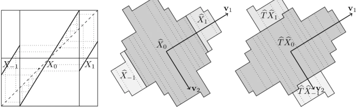
In Figure 3, we can see the transformation and the orbits of−α, αon the left, the natural extension domainXb and its decomposition intoXba,a∈A, as well as the setsJx− Dx,x∈ V, in the middle,
and the decomposition of TbXb on the right. Since Te5α = T5α = .(0001)ω 6∈ V, there is no
dotted line for this point in the natural extension domain. The point lies between the first and second dotted line, counted from the origin in the direction of v1 and is the point above which
the boundary between TbXb1 and TbXb0 makes the step. That this point is not in V implies that
Dx does not change here, but we can see that the shape of the sets TbXb1 and TbXb0 changes.
This means that the decomposition of Dx according to (14) changes here. The same happens at
e
T5(
−α) =T5(
−α) =.(000¯1)ω withTbXb
X−1 X0 X1
b
X−1 b
X0
b
X1 v1
v2 b
TXb−1 b
TXb0 b
TXb1
v1
v2
Figure 3. The transformation from Example 3.15 and its natural extension.
Example3.16. LetT be the symmetricβ-transformation for the golden ratioβ, i.e.,A={−1,0,1}, X−1=
−1 2,−
1 2β
, X0=
− 1 2β, 1 2β
X1=
1
2β, 1 2
, see Example 2.12. We have
T4 −1 2β
=T3 −1 2
=T2 1 2β2
=T 2β1= −21, Te4 1 2β
=Te3 1 2
=Te2 −1 2β2
=Te −2β1= 12, thusV =−1
2,− 1 2β,−
1
2β2,2β12,2β1 . The transformation and its natural extension are depicted in
Figure 4. Note that0is a repelling fixed point of the transformation. Here, this implies that, for allx∈[− 1
2β2,2β12), the only sequence w∈
ωAsuch that w
·b(x) isT-admissible is · · ·00. Hence, Dx={0} for allx∈[−2β12,2β12).
When we construct a multiple tiling forT, we want to disregard these sets and we achieve this by restrictingT to the support of its invariant measureµ, which is the set [−1
2,− 1
2β2)∪[2β12,12).
If we restrictT to this set,T is a right-continuousβ-transformation of which the domainX is not a half-open interval. The setX0 is split into two parts as well.
For other values ofβ, we refer to Section 4.5.
X−1 X0 X1
b
X−1 b X0 b X0 b X1 v1 v2 b
TXb−1 b
TXb0
b
TXb0 b
TXb1 v1
v2
Figure 4. The transformation from Example 3.16 and its natural extension.
Example 3.17. We will see in Section 4 thatλ2(Xb) = 1 in Examples 3.14–3.16. For a
transforma-tion withλ2(Xb)>1, letβbe again the golden ratio, nowA=
{−1,1},X−1= [−1,0),X1= [0,1).
ThenTe3(0) =Te2(1) =Te(1/β) = 0,T3(0) =T2(
−1) =T(−1/β) = 0, thusV ={−1,−1/β,1/β}, see Figure 5.
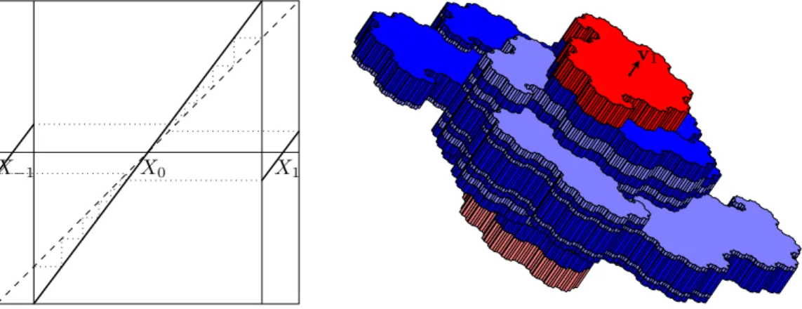
Example 3.18. Consider now a minimal weight transformation with the Tribonacci number β, which is the real solution of the equation x3
−x2
−x−1 = 0. Choose α = 1
β+1, i.e., let
A={−1,0,1},X−1=
−β β+1,β+1−1
,X0=
−1
β+1,β+11
, X1=
1
β+1, β β+1
. Then ˜b(−α) = ¯1(010)ω,
b(−α) = (0¯10)ω, ˜b(α) = (010)ω, b(α) = 1(0¯10)ω, thus
X−1 X1
b
X−1 b
X1 v1
v2 TbXb
−1 b
TXb1 v1
v2
Figure 5. The transformation from Example 3.17 and its natural extension.
X−1 X0 X1
v1
Figure 6. The transformation from Example 3.18 and its natural extension domain.
Example3.19. Ifβis the smallest Pisot number, i.e., the real solution of the equationx3
−x−1 = 0, then α= ββ8−61 provides a minimal weight transformation as in Example 3.18. We have ˜b(α) =
(0106)ω, b(α) = 1(06¯10)ω, thus
V =β±8β−k1 : 0 ≤k ≤ 7} \
β7
β8−1} since ˜b(−α) and b(−α) are
obtained by symmetry fromb(α) and ˜b(α). See Figure 7.
X−1 X0 X1
v1
4. Tilings
In this section, we consider two types of (multiple) tilings which are closely related. The first one is an aperiodic (multiple) tiling of the hyperplane H by setsDx defined in (9). The second
one is a periodic (multiple) tiling ofRd by the closureYb of the natural extension domainXb. As for the natural extensions,T is a right-continuousβ-transformation andβ a Pisot unit. We furthermore assume that A ⊂Z[β], i.e., that q= 1 in Lemma 3.5, and that the set V, which is defined in (10), is finite.
4.1. Tiling of the contracting hyperplane. We define tiles in the hyperplaneH by Tx= Φ(x) +Dx for all x∈Z[β]∩X,
with Φ as in (7) andDx as in (9).
Remark 4.1. The tiles are often defined inRr×Cs, whereris the number of real conjugates and
2sis the number of complex conjugates ofβ. We clearly haveRr×Cs≃H. We choose to work inH because many statements are easier to formulate inH than in Rr×Cs.
The familyT ={Tx}x∈Z[β]∩Xis amultiple tiling of the spaceH if the following properties hold.
(mt1) There are only finitely many different setsDx, and these sets are compact.
(mt2) The familyT islocally finite, i.e., for everyy∈H, there is a positiversuch that the set {x∈Z[β]∩X : Tx∩B(y, r)6=∅}is finite.
(mt3) T gives a covering ofH: for everyy∈H, there is a tileTx, such thaty∈ Tx.
(mt4) Every setDx, x∈Z[β]∩X, is the closure of its interior.
(mt5) There is an integerm≥1 such that almost all points ofH are in exactlymdifferent tiles. The numbermis called thecovering degree of the multiple tiling.
Atiling is a multiple tiling with covering degree 1.
The tilesTx, x∈Z[β]∩X, are translates of a finite collection of compact sets by Lemma 3.8,
Proposition 3.9 and the finiteness ofV. This proves (mt1). An important tool for showing (mt2)– (mt5) will be that the set of translation vectors, Φ(Z[β]∩X), is aDelone set in H, i.e., that it is uniformly discrete and relatively dense inH. Precisely,
• A set Z is relatively dense in H if there is an R > 0, such that, for every y ∈ H, B(y, R)∩Z6=∅.
• A set Z is uniformly discrete if there is an r > 0 such that, for every y ∈ Z, the set B(y, r)∩Z contains only one element.
In [Moo97], Moody studied, among other things, Delone sets. He gave a detailed exposition of Meyer’s theory, which was developed in [Mey72]. According to Meyer, model sets for cut and project schemes are Delone. We will use this to prove Lemma 4.3. We also need the following lemma.
Lemma 4.2. The map Φ : Q(β)→H is injective.
Proof. Recall that Φ(x) = Ψ(x)−xv1, and that Ψ : Q(β)→Qdis bijective by Lemma 3.4. Since
the coefficients ofv1 are linearly independent overQ, Φ is injective.
Lemma 4.3. Every set Φ(Z[β]∩E), where E ⊂ R is bounded and has non-empty interior, is uniformly discrete and relatively dense. In particular, this holds forΦ(Z[β]∩X).
Proof. By Proposition 2.6 from [Moo97], it suffices to show that Φ(Z[β]∩E) is a model set. Define the projectionπH : Rd →H byπH(x) =x−π1(x)v1, with π1 as in Section 3.1, and
set ι(x) = (πH(x), π1(x)). Then the pair (H×R, ι(Zd)) is a cut and project scheme, sinceι(Zd)
is a lattice,πH is injective onZd,π1(Zd) =Z[β] is dense in RandH ≃Rd−1. The injectivity of
πH onZd follows again from the linear independence of the coefficients ofv1 overQ.
is a model set, and therefore a Delone set by Proposition 2.6 from [Moo97].
Corollary 4.4. The family {Tx}x∈Z[β]∩X is locally finite.
Proof. This follows immediately from the uniform discreteness of Φ(Z[β]∩X), the injectivity of Φ
and the fact thatkϕ(w)k,w∈ωA, is bounded.
Hence we have (mt2). The next lemma gives (mt3).
Lemma 4.5. We have H=Sx∈Z[β]∩XTx. Proof. Let H′ = S
x∈Z[β]∩XTx. Every point y ∈ H′ is of the form y = Φ(x) +ϕ(w), with
x∈Z[β]∩X, w∈ωA,w·b(x)∈ S. We have Mβy =ϕ(wb1(x)) + Φ(T x), withT x∈Z[β]∩X
sinceb1(x)∈Z[β], and thusMβy∈H′. Hence,MβH′ ⊆H′. SinceT is surjective, every tile Tx,
x ∈ Z[β]∩X, is non-empty. By Lemma 4.3 and since ϕ(w) is bounded, H′ is relatively dense in H. Since MβH′ ⊆H′ and Mβ is contracting on H, H′ is dense inH. By the compactness of
the tiles and the local finiteness ofT, we obtainH′=H.
Now, we can prove that the boundary of every tile has zero measure. This generalizes Theorem 3 in [Aki99].
Proposition 4.6. We have λd−1(∂
Dx) = 0 for everyx∈X. Proof. If λd−1(D
x) = 0, then λd−1(∂Dx) = 0 since Dx is compact. Therefore, we can assume
λd−1(D
x)>0. We first show thatλd−1(∂Dy) = 0 for somey ∈X withλd−1(Dy)>0, and then
extend this property to arbitraryx∈X.
SinceH=Sz∈Z[β]∩XTz, there exists, by Baire’s theorem, somez∈Z[β]∩X such thatTz, and
thusDz, has an inner point (with respect toH). By iterating (14), we obtain for all k≥1 that
Dz is the (up to sets of measure zero) disjoint union ofMβkDy+ϕ(b1(y)· · ·bk(y)), y ∈T−k{z}.
SinceMβ−1 is expanding onH, there must be somey ∈T−k
{z} for sufficiently largeksuch that Mk
βDy+ϕ(b1(y)· · ·bk(y)) is contained in the interior ofDz, andλd−1(Dy)>0. Then every point
in ∂(Mk
βDy+ϕ(b1(y)· · ·bk(y))) lies also in MβkDy′ +ϕ(b1(y′)· · ·bk(y′)) for some y′ ∈ T−k{x},
y′6=y. Since the intersection of these sets has zero measure, we obtainλd−1(∂D y) = 0.
Now, consider a setMβDz+ϕ(b1(z)),z∈T−1{y}, in the subdivision ofDy. Every point on the
boundary of this set is either also on the boundary of another set from the subdivision, or not. If not, then the point is in∂Dy. Therefore, we haveλd−1(∂Dz) = 0 for everyz∈T−1{y}. It remains
to show that, when iterating this argument, everyDxwithλd−1(Dx)>0 occurs eventually in one
of these subdivisions. By Proposition 3.9, it is sufficient to considerx∈ V.
Similarly to the graph of the GIFS, let G be the weighted directed graph with set of vertices V′ =
{x∈ V: λd−1(
Dx)>0} and an edge fromxtox′ if and only ifT−1Jx∩Jx′ 6=∅. Then we haveλd−1(∂D
x′) = 0 for every x′ ∈ V which can be reached from the vertex xsatisfyingy∈Jx.
Let the weight of an edge beλd(Tb−1(Jxv1− Dx)∩(Jx′v1− Dx′))>0. SinceTb is bijective off of a set of Lebesgue measure zero, the sum of the weights of the outgoing edges as well as the sum of the weights of the ingoing edges must equalλd(J
xv1− Dx) for everyx∈ V′. This implies that
every connected component ofG must be strongly connected, in the sense that if two vertices are in the same connected component, then there is a path from one vertex to the other and the other way around.
LetC be a (strongly) connected component ofG and X′ =S
x∈CJx. For everyz ∈Jx, x∈ C,
DT z containsMβDz+b1(z), thusλd−1(DT z)>0, henceT z∈X′. Therefore, the restriction ofT
toX′ is a right-continuousβ-transformation, and this restriction changes everyD
x,x∈X′, only
by a set of measure zero. The arguments of the preceding paragraph provide somey ∈X′ with
λd−1(∂
Dy) = 0, and we obtainλd−1(∂Dx) = 0 for allx∈X′, thus for allx∈X.
If we want that (mt4) holds, then we clearly have to exclude non-empty tiles of measure zero. This means thatX has to be the support of the invariant measureµ=λd
◦π−1, which is defined
in Section 3.1. Note that restrictingT to the support ofµchanges the tiles only by sets of measure zero.
Lemma 4.7. If the support of the invariant measureµisX, then Dx= int(Dx)for everyx∈X.
Proof. Since the tiles are compact, we have int(Dx) ⊆ Dx for every x ∈ X. For the other
inclusion, we show that Tx ⊆int(Tx) for every x∈ Z[β]∩X. If y∈ Tx, then y = Φ(x) +ϕ(w)
for some w = (wk)k≤0 ∈ ωA with w·b(x) ∈ S. Set xk = .w−k+1· · ·w0b(x) for k ≥ 0. Then
Mk
β(Φ(xk)+Dxk)⊆ Tx. We haveλd−1(Dxk)>0 since the support ofµisX. Also,λd−1(∂Dxk) = 0
by Proposition 4.6. Therefore, there exists a pointyk ∈Mβk(Φ(xk) + int(Dxk))⊆int(Tx). Since
limk→∞yk =y, we havey∈int(Tx).
The familyT isself-replicating, i.e., for each elementTx ofT, we can writeMβ−1Tx as the (up
to sets of measure zero) disjoint union of elements fromT. By Lemma 3.13, we have
(16) Mβ−1Tx=Mβ−1
Φ(x) + [
y∈T−1{x}
MβDy+ Φ b1(y)
= [
y∈T−1{x}
Ty.
Fory∈H andr >0, thelocal arrangement inB(y, r) is the set
P B(y, r)=Tx∈ T : Tx∩B(y, r)6=∅ .
As a next step in proving that the family T is a multiple tiling, we will show that T is quasi-periodic, i.e., for anyr >0, there is anR >0 such that, for anyy,y′
∈H, the local arrangement inB(y, r) appears up to translation in the ballB(y′, R).
Proposition 4.8. The family T is quasi-periodic.
Proof. Note first that, for eachr >0, there are only finitely many different local arrangements up to translation, since Φ(Z[β]∩X) is uniformly discrete and there are only finitely many different setsDx.
Letr >0. If two tilesTx andTx+y are in the same local arrangement, then
(17) kΦ(y)k<2(r+ max
w∈ωAkϕ(w)k
and y∈X−X.
By Lemma 4.3 and since Φ is injective, the set of elementsy ∈Z[β] satisfying (17) is finite. Call this setF, and note that 0∈F.
Now, take some local arrangementP(B(y, r)) and x∈ Z[β]∩X such that Tx ∈ P(B(y, r)).
For anyy ∈F, ifx+y∈X, then there is anεy >0 such thatJx+y = [x+y, x+y+εy), and if
x+y6∈X, then there is anεy>0 such that [x+y, x+y+εy)∩X =∅. Letε= miny∈Fεy and
consider somez∈Z[β]∩[0, ε). For anyy∈F, we have eitherx+y∈X andTx+y+z=Tx+y+ Φ(z)
sinceDx+y+z=Dx+y, orx+y6∈X andx+y+z6∈X. Therefore,P(B(y+ Φ(z), r)) is equal to
P(B(y, r)), up to translation by Φ(z).
By Lemma 4.3, Φ(Z[β]∩[0, ε)) is relatively dense in H. Thus, every local arrangement occurs relatively densely inH. Since the number of local arrangements is finite, the lemma is proved.
Lemma 4.5 implies that everyy∈H lies in at least one tile. By the local finiteness ofT, there exists anm≥1 such that every element ofH is contained in at leastmtiles inT and there exist elements ofH that are not contained inm+ 1 tiles. For thism, a pointy∈H lying in exactlym tiles is called an m-exclusive point. A point lying in exactly one tile is called an exclusive point. Similarly to [IR06], we obtain the following proposition, which gives (mt5).
Proposition 4.9. There exists anm≥1 such that almost everyy∈H is contained in exactlym
tiles.
Proof. We first show that the set of points that do not lie on the boundary of a tile is open and of full measure. LetC=Sx∈Z[β]∩X∂Txdenote the union of the boundaries of all the tiles inT.
This set is closed, since it is the countable union of closed sets that are locally finite. Hence,H\C is open. By Proposition 4.6, we also haveλd−1(C) = 0.
Letm be as in the paragraph preceding the proposition, andx∈H be anm-exclusive point, lying in the tilesTx1, . . . ,Txm. Since the tiles are closed, there is anε >0 such thatB(x, ε)∩Tx=∅