Do we follow others when we should? A simple test of
rational expectations
1Georg Weizsäcker
London School of Economics and Political Science
April 2008
Abstract: The paper presents a new meta data set covering 13 experiments on the social learning games by Bikhchandani, Hirshleifer, and Welch (1992). The large amount of data makes it possible to estimate the empirically optimal action for a large variety of decision situations and ask about the economic signi…cance of suboptimal play. For example, one can ask how much of the possible payo¤s the players earn in situations where it is empirically optimal that they follow others and contradict their own information. The answer is 53% on average across all experiments –only slightly more than what they would earn by choosing at random. The players’ own information carries much more weight in the choices than the information conveyed by other players’ choices: the average player contradicts her own signal only if the empirical odds ratio of the own signal being wrong, conditional on all available information, is larger than 2:1, rather than 1:1 as would be implied by rational expectations. A regression analysis formulates a straightforward test of 1
I am grateful for helpful comments by Mohit Bhargava, Stefano DellaVigna, Erik Eyster, Bernardo Guimaraes, Dorothea Kübler, Luke Miner, Charles Noussair, Matthew Rabin, Myung Seo and seminar audiences at Berkeley, Copenhagen and MPI Bonn. Mohit Bhargava and Luke Miner also provided excellent research assistance. The collection of the meta data set was made possible by Jonathan Alevy, Lisa Anderson, Antonio Guarino, Charles Holt, Angela Hung, John List, Markus Nöth, Clemens Oberhammer, Joerg Oechssler, Brian Rogers, Andreas Roider, Andreas Stiehler, Martin Weber and Anthony Ziegelmeyer who provided the individual data sets. Finally, I thank the ESRC (Award RES-000-22-1465) for funding.
rational expectations, which rejects, and con…rms that the reluctance to follow others generates a large part of the observed variance in payo¤s, adding to the variance that is due to situational di¤erences.
Keywords: Social learning, information cascades, failure of rational expectations, meta analysis
JEL Classi…cation: C72, C92, D82
Contact: [email protected]
1
Introduction
The paper re-visits the experimental literature on social learning and addresses a signi…cant gap in the existing data analyses: to what extent is it bene…cial for a decisionmaker to learn from others and contradict his or her own private information – and if it is bene…cial, do people do it? These questions lie at the heart of understanding social learning behavior but have been answered only very partially. The main di¢ culty in …nding appropriate answers is the identi…cation of conditions under which a decisionmaker should follow others. Most previous discussions in the literature measure a decisionmaker’s success under the assumption that other players obey a given model solution, e.g. Bayes Nash Equilibrium or Quantal Response Equilibrium. Any such theory implies an optimal response of the decisionmaker herself, which can be held against the data.2 But despite the undisputable usefulness of these solutions, it is important to note that they are often inaccurate and thus their implications are imperfect benchmarks. It has never been established to what degree the decisionmakers choose the empirically optimal action, i.e. the action that is ex-post optimal most of the time under identical conditions. This paper’s premise is that the empirically optimal action is what we should measure the success of social learning by, because it re‡ects all relevant situational factors, including those that are in‡uenced by the true behavior of other players. The paper combines the raw data from a large set of experiments (all of which follow Anderson and Holt, 1997) into a new meta data set and asks whether the average behavior can be viewed as approximately payo¤ maximizing, given the behavior of others. It …nds that the success of learning from others is very modest. Conditional on being in a situation where it is empirically optimal for the participants to contradict their own private information, they choose this action (among two
2
Anderson and Holt (1997), the in‡uential …rst study in this experimental literature, contains a data analysis using both Bayes Nash Equilibrium and Quantal Response Equilibrium. Most subsequent studies have summarized behavior on the equilibrium path of Bayes Nash Equilibrium, see e.g. the survey in Kübler and Weizsäcker (2005). Variants of Quantal Response Equilibirum are discussed in Oberhammer and Stiehler (2003), Kübler and Weizsäcker (2004), Choi, Gale, and Kariv (2004), Drehmann, Oechssler and Roider (2005), Krämer, Nöth and Weber (2006) and Goeree et al (2007).
alternatives) in less than half of the cases.3 On the other hand, in cases where their own signal happens to support the empirically optimal action, the participants more likely realize this and follow the signal nine out of ten times.
These and all other results in the paper are generated under a reduced-form approach, without imposing a behavioral model of the players’ decisionmaking process or a model of how they take other players’actions into account. (For example, the analysis does not assume that players apply Bayesian updating.) A disadavantage of not imposing a behavioral model is that we learn little about the nature of the suboptimality. Yet the results are supportive of the model estimates by Nöth and Weber (2003) and Goeree et al (2007), which suggest that people assign too much weight to their own private information, relative to the publically observable choices of others.4
But can the high error rate perhaps be attributed to the lack of strong incentives? Especially in situations where a player receives a signal that is di¤erent from other players’ signals, the expected gain from making correct inferences is reduced: with con‡icting pieces of information, the total value of the available information is small and all choice options are unsuccessful with relatively high likelihood. This makes it less important to choose the best option. At the same time, players may also …nd it more di¢ cult to identify the optimal action in situations with con‡icting information. One may thus expect a positive correlation between simplicity and lucrativity (value of the available information) of choice situations. The mere choices frequencies may therefore be misleading indicators of success if they do not consider the di¤erences in the importance of making the optimal choice –the players may do the right thing predominantly when it is important.5
3The frequency is about 0.44 and depends on the set of included cases – the identi…cation of the empirically optimal action relies on small sample sizes for many decision problems so that it is better not to include these cases (see Section 3). But for any of a large selection of possible sets, the frequency lies below one half.
4These and other reports of biases relative to a rational-expectations benchmark (Oberhammer and Stiehler, 2003, Kübler and Weizsäcker, 2004, Kraemer, Nöth and Weber, 2006) are essentially con…ned to establishing statistical signi…cance. The existing literature has largely sidestepped a detailed discussion of payo¤ outcomes – as opposed to behavioral outcomes – and most studies merely contain measures of overall earnings in the experiment. A notable exception is in Goeree et al’s (2007) discussion of higher average earnings of players who choose later in the game.
5
The complication is particularly severe in social learning games, where uncertainty about others’strategies prevails so that the value of the available information (here, the observation of others’actions) is unknown to the researcher.
But with enough data one can estimate the value of the available information and control for it in the analysis. Below, calculations will show that the success rate indeed increases with the importance of making the optimal choice, but still social learning is unsuccessful in payo¤ terms. In situations where participants should contradict their own signal, they only receive 53% of the higher of the two possible prizes on average (normalizing the low prize to zero). They could have earned 64% of the high prize on average, had they always realized that it is better to contradict their own information. In contrast, in the complementary set of situations, where it is empirically optimal for participants to follow their own information, they are much more successful and earn 73% of the high prize on average, out of 75% that they could earn from always behaving optimally. Indeed, the numbers show that the latter set of situations is more lucrative for the players, but also that the di¤erence in success rates generates a large payo¤ gap.
Estimating the value of the players’information is particularly straightforward in games like the present ones, where there are only two payo¤ outcomes and two available actions for each player. One can simply count how often each of the two actions would have yielded the higher of the two possible prizes, across all instances where the available information is identical.6 The relative frequency of the two counts then yields the desired estimate. This exercise is applied to the new data set consisting of data from 13 di¤erent experimental studies on the game by Bikhchandani, Hirshleifer, and Welch (1992), which is widely viewed to capture the essence of social learning. All of these experiments follow the same format, with only minor modi…cations and di¤erences in the experimental procedures, such as di¤erent precisions of signals. The data set contains a large variety of di¤erent decision situations –there are more than 10000 distinct decision problems if one counts decisions in di¤erent experiments separately, and almost 30000 decisions in total –but all of them are generated within the same basic game, with two possible states of the world and two actions per player, and they can therefore be summarized in meaningful ways. Section 3 describes the statistical connection between the participants’ frequency of following their own information and the estimated value of this action. This description demonstrates a strongly in‡ated tendency of
6
As will be made clear in Section 2, this estimation only views situations as identical if their informational conditions are the same and if they appear in the same treatment of the same experiment.
participants’to follow their private information, and indeed gives a negative answer to the question in the paper’s title, as described above: when participants should optimally contradict their own signal, this action is observed in less than half of the cases. As the value of this action increases, its frequency increases, but at a slow rate. To observe a frequency of one half or more, the action’s value needs to exceed 2/3 of the higher prize. That is, to induce the average participant to act against her signal, the evidence conveyed by the other players’decisions needs to be so strong that even after accounting for the countervailing signi…cance of the signal, the empirical likelihood ratio against the signal is larger than 2:1.
The reader may note that the above classi…cation of situations –whether or not the own signal supports the empirical optimal action – makes for an unusual explanatory variable because it is unobservable to the decisionmaker. But of course, it is correlated with other, more transparent classi…cations. Section 4 considers an natural one, whether or not a player’s signal is in contradiction to a strict majority of previous players’choices. This variable and the success rates under each of its categories are highly correlated with the above-described results,7 indicating again that people underestimate how much information is contained in other people’s choices. There is also a positive e¤ect of unanimity of previous choices: participants are much more successful in learning from others if the others all agree.
Section 4 presents these results in a regression analysis that projects the observed behavior on explanatory variables that describe the nature of the situation. Importantly, one of the control variables is the value of the empirically optimal choice. If this value is held constant, and under the assumption of rational expectations, there is no reason for a systematic behavioral change in response to the nature of the situation. The signi…cance test for the other explanatory variables therefore makes for a straightforward consistent test of the hypothesis that players respond to rational expectations. The test rejects strongly: the behavioral change depending on whether the own signal contradicts the majority of previous choices is highly signi…cant and accounts for about
7
The average earnings are 55% of the high prize in situations where the own signal contradicts the majority; were the participants to choose the empirically optimal action in each case, they would earn 65% in these situations. In the remaining situations, where the signal coincides with the majority of previous choices – so that the bias in favor of the own signal may help the participants – they earn 72% out of the maximum feasible payo¤ of 75%.
half of the total payo¤ di¤erences between the two classes of situations.
Section 5 concludes with a discussion of how the methodology may be applied in other data contexts. It argues that the identi…cation of empirically optimal actions can be used generally in tests of rational expectations models, if enough data is available.
2
A meta data set of cascade game experiments
Anderson and Holt’s (1997) experiment was replicated and modi…ed by numerous researchers, and the new meta data set is restricted to this class of experiments because the structure of the game is thereby held constant in all subsets of data.8 The following describes the game with Anderson and Holt’s speci…c parameter values. At staget= 0, Nature draws one of two states of the world, ! 2 fA; Bg, withPr(A) = 0:5. The states are represented by two urns labelled A and B. Of the balls in urnA, a fractionqA= 2=3 is labelledaand 1 qA is labelledb. Urn B, analogously,
has fractions of qB = 2=3 labelled b and 1 qB labelleda. Nature’s draw is not revealed, so that
it is unknown in the remainder of the game whether balls are chosen from AorB. A set ofT = 6 players makes predictions about this event. At staget= 1, the …rst player receives a private signal, in the form of a ball drawn from the true urn. The player then predicts the state of the world, i.e. chooses an action d2 . At t= 2, the next player receives a signal from the same urn, makes a prediction, and so on until the game ends after stageT. If a player’s prediction coincides with the true urn, she gets a …xed amount U, here normalized to1. Otherwise, the player gets 0.9 Social learning is possible because att 2the players observe the predictions made by all previous players 1; :::; t 1 (but not their signals). Hence, players can make their choices dependent on the choices
8
Other social learning experiments are those on learning in networks (e.g. Choi, Gale, and Kariv, 2004), on cascade games that do not follow the Anderson/Holt format (Allsopp and Hey, 2000, Celen and Kariv, 2004, Guarino, Harmgart and Huck, 2007) and games where agents are replaced by groups (Fahr and Irlenbusch, 2008). Several papers also address how experimental participants play social learning games against automated opponents with exogenously …xed behavior (Huck and Oechssler, 1999, Grebe, Schmidt and Stiehler, 2006, Kraemer, Nöth and Weber 2004).
9
Note that since there are only two possible payo¤s for each player, risk considerations would be absent under any expected-utility model.
of other players. Information cascades can arise in Bayes Nash Equilibrium: e.g., if the …rst two players make an identical prediction, say,A, then in sequential equilibrium the third player chooses Aeven if she has signalb. The fourth player, too, follows the prediction of the initial three players, and so on for later players. Quantal Response Equilibrium and its variants also prescribe that the decision makers learn from the predecessors’choices, and tend to follow them.
Anderson and Holt played the game with 18 participants, each of whom took part in 15 repeti-tions of the game, with randomly changing player posirepeti-tions between the repetirepeti-tions. In a separate asymmetric treatment, 36 subjects played a modi…ed version (again with 15 repetitions), where the proportion ofaballs in urnAisqA= 6=7, and the proportion ofbballs in urnB isqB= 2=7. Both
treatments are used in the analysis, yielding a total number of N = 810 decisions. The following lists the other data sources:
Willinger and Ziegelmeyer (1998, N = 324). Basic (symmetric) Anderson/Holt experiment, withq qA=qB= 0:6, 36 participants, and 9 repetitions.
Anderson (2001,N = 270). Symmetric Anderson/Holt experiment, with q 2=3, 18 partici-pants, and 15 repetitions.
Hung and Plott (2001,N = 890). Replication of Anderson/Holt withT = 10and q= 2=3, in three treatments with minor di¤erences in the experimental implementation. 40 participants and 22:25repetitions on average.
Ziegelmeyer et al (2002, N = 810). 54 participants and 15 repetitions with T = 9, Pr(A) = 0:55and q= 2=3. Subjects in one of the two treatments also reported beliefs about the state of the world.
Nöth and Weber (2003, N = 9834). Variant of the game with T = 6, where q is drawn for each player from f0:6;0:8g, in independent draws with equal probabilities, and the realized signal precision is known to the player herself but unknown to other players. 126participants and about 78repetitions on average.
Oberhammer and Stiehler (2003, N = 876). Variant where subjects also announce their
willingness to pay for playing the game, with T = 6, q = 0:6,36 participants, and about 24 repetitions on average.
Kübler and Weizsäcker (2004, N = 482). Variant where subjects also decide whether or not to receive a private signal, this decision not being revealed to other players. 36 participants and 15 repetitions, withT = 6 and q = 2=3. 68 observations are dropped from the original data, in cases where the corresponding participants requested no signal.10
Dominitz and Hung (2004, N = 2270). 90 participants, games with T = 10 and q = 2=3. 30 participants played 20 regular repetitions, and the other 60 participants reported belief statements during the last10 out of 20 repetitions.
Cipriani and Guarino (2005, N = 161). Variant where players have an outside option, mod-elled after the possibility not to trade in …nancial markets. 48participants and10repetitions, with T = 12 and q = 0:7. 319 observations are dropped from the original data because the participant or one of her predecessor chose the outside option.11
Drehmann, Oechssler and Roider (2005, N = 2789) 1840 participants played in 8 di¤erent Internet-based treatments with di¤erent signal precisions and di¤erent values forPr(A). 267 participants were management consultants who played among each other, with T = 7. In addition,1573participants of di¤erent backgrounds (mostly students or graduates of univer-sities) played in games withT = 20(mostly). Participants played up to three repetitions.
Alevy, Haigh and List (2006, N = 1647). Replication of both Anderson/Holt treatments, withT = 5 orT = 6,15 repetitions, and with subjects of di¤erent backgrounds: 55 …nancial market professionals, and 54 undergraduate students. Treatments also di¤ered with respect to gains/losses framing. Eight treatments in total.
1 0Receiving a signal is weakly dominant in this game.
1 1For risk-neutral expected-utility maximizers, the outside option is strictly suboptimal for almost all subjective beliefs that a player may have about the state of the world. This game is the only game with three possible payo¤s, so that risk considerations may become important. For the sake of completeness, I decided to include the (few) data despite these di¤erences.
Goeree et al (2007, N = 8760). 380 participants play in four long-game treatments, with T = 20and T = 40,q = 5=9 and q= 2=3, and an average of 22:7repetitions.
In total, the meta data set contains 29923individual decisions fsig29923i=1 , made by 2813 partici-pants in13 separate studies. All of them follow the observation of a private signal and a (possibly empty) string of previous choices made in analogous situations. In all of them there are two actions and two possible payo¤s,12 but the data set nevertheless contains decisions with a large variety in environments, instructions, and histories of other players’choices.
Frome here on, let a "decision"si be a row in the data matrix –a vector of variable realizations
that describe a partipant’s choice problem in one particular repetition of a game. Each decisionsi
in the data set contains the description of the game (Pr(A)i; qA;i; qB;i; Ti), the participant’s player
position ti, her choicedi and the true state of the world!i.13 In addition, the following variables
are contained insi:
groupi: An identifying variable that denotes the group of participants with whom the
partici-pant played the current repetition of the game.14
treatmenti: A categorical variable that de…nes two decisions (si; sj) to be in the same
treat-ment if (i) the participants received the same instructions for the current game, and (ii) the par-ticipants (and their opponents) are drawn from the same pool.15
Ii (information): A set of variables describing the history of play in the current repetition of
the game, including all previous choices as well as the participant’s signal. E.g. if the participant 1 2
But with the quali…er about Cipriani and Guarino (2005) – see the previous footnote. 1 3Information on!
iis available for each decision –which is crucial for estimating the empirical value of each action
–thanks to the "no-lying-to-subjects" policy in experimental economics: all urn and signal draws in the experiments were actually made according the described process, and not made up by the experimenters.
1 4
With the exception of the Internet-based experiment by Drehmann, Oechssler and Roider (2005), the matching of participants into groups remained constant throughout all experiments, so that no participant was part of several groups.
1 5
This does not require identical conditions for other parts of the experiment, e.g. for the belief elicitation in some studies or for the number of repetitions of the game. In all cases except one, this treatment de…nition coincides with that of the original studies’treatment de…nitions (the exception is Dominitz and Hung, 2004, who had two treatments with di¤erent belief elicitation procedures). But most studies included additional treatments.
in decision si acts as the …rst player in the game, she may have Ii =a, or if she acts as the third
player she may have Ii =ABa. In the case of the Nöth/Weber dataset where the signal strength
di¤ers between the participants, the information about the own signal strength is also part ofIi.16
contradicti: An indicator of whether or not the participant in decision si contradicts her own
signal –e.g. choosesd=Awith own signal b.17
sitcounti: A counting variable that contains the number of times that a decision with the same
information Ii occured within the same treatment. In treatments with A=B symmetry (Pr(A) =
0:5; qA =qB), this includes situations with the symmetric information set. (E.g. AABa is viewed
as identical toBBAb.)
Let Se(si) be the set of all decisions that are identical to si, in the sense that the (treatmenti,
Ii)-description is the same. By de…nition, sitcounti = jSe(si)j. Further, let Se fSekgk be the
resulting set of all distinct sets of identical situations: each element of Se is a set of identical decisions and eachsi appears in one and only one element ofSe. Notice that these de…nitions ignore
information about history of play in previous repetitions of the game, i.e. they pool situations as identical across di¤erent histories. The subsequent analysis relies on this pooling and thereby makes the simplifying assumption that pre-current-game history does not enter into a participant’s decisionmaking process.18 Under this assumption it holds that the decisionmaking process in decision si – whatever it may be – uses only information that is identical across Se(si) because
all that the participants learn about the random draws or about the possible characteristics of other players is re‡ected in (treatmenti, Ii).19 The following variable estimates the value of this
1 6
In e¤ect, there are four di¤erent signals in this data set: a weak; a strong; b weakandb strong. 1 7
For this de…nition to apply also in the case of the Nöth/Weber experiment where there are four signals, the phrase "contradicts her own signal" is to be understood e.g. as a choice ofB after observing a signal a weak or
a strong.
1 8The assumption is restrictive but still relatively mild: it is di¢ cult to learn about other player’s strategies in social learning games because their signals remain unknown and player positions change after each repetition of the game. Several studies (e.g. Kübler and Weizsäcker, 2004) looked for behavioral changes over the course of the experiments and found at most weak changes. The meta data set allows for further checks, which support the assumption. For example, the frequency of following the own signal changes by 0.6 percentage points between the …rst and the second half of the experiments (0.767 versus 0.761).
1 9
information, using the ex-post knowledge about !i, the true underlying state of the world. It is
the key ingredient of the analysis –the empirical value of contradicting one’s signal.
mean_payjcontradicti: Averaging across situations sj 2Se(si), the payo¤ that the
partici-pant earns if she chooses contradicti=1. Due to the payo¤ normalization, this variable is identical
to the frequency acrosssj 2Se(si)of the participant’s signal being wrong, i.e. the state of the world
!j not being indicated by the signal.
The variable mean_payjcontradicti is an average of a …nite sample. As sitcounti increases, this
average approaches the mean of the corresponding random variable, i.e., it approaches the expected payo¤ from contradicting one’s signal, conditional on all available information. This conditional expected payo¤ is what that the player should care about: she should contradict her signal if the expected payo¤ from doing so exceeds0:5.
For small sitcounti, however, mean_payjcontradicti may be far away from its expected value. I
will therefore restrict attention to cases where there are strictly more than 10 occurances of identical situations in the data set, i.e. where sitcounti = jSe(si)j > 10. Almost half of the decisions are
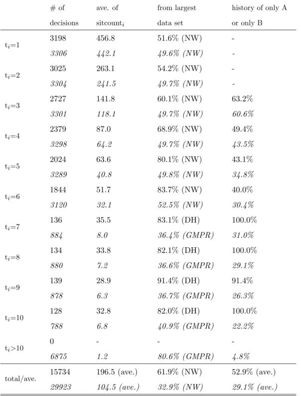
therefore not considered in the statistical analysis: out of the 29923 situations, 15734 remain in the restricted data set. To give the reader an impression of the resulting selection of the subsample as well as a general overview of the data, the following two tables present some features of the restricted data set (…rst entry in each cell) and the full data set (second entry, in italics). Table 1 organizes the data by decisionsfsigi, and Table 2 by distinct decisionsfSekgk(so that each distinct
decision counts only once for the reported values in Table 2).
anonymity between the participants during the experiment. If participants can observe each other’s person-speci…c characteristics, there are informational di¤erences even withinSe(si)– but these should be minor. Another caveat is
that unobservable di¤erences between experimental sessions within the same treatment cannot be taken into account.
# of decisions ave. of sitcounti from largest data set
history of only A or only B ti=1
3198 3306 456.8 442.1 51.6% (NW) 49.6% (NW) -ti=2
3025 3304 263.1 241.5 54.2% (NW) 49.7% (NW) -ti=3
2727 3301 141.8 118.1 60.1% (NW) 49.7% (NW) 63.2% 60.6% ti=4
2379 3298 87.0 64.2 68.9% (NW) 49.7% (NW) 49.4% 43.5% ti=5
2024 3289 63.6 40.8 80.1% (NW) 49.8% (NW) 43.1% 34.8% ti=6
1844 3120 51.7 32.1 83.7% (NW) 52.5% (NW) 40.0% 30.4% ti=7
136 884 35.5 8.0 83.1% (DH) 36.4% (GMPR) 100.0% 31.0% ti=8
134 880 33.8 7.2 82.1% (DH) 36.6% (GMPR) 100.0% 29.1% ti=9
139 878 28.9 6.3 91.4% (DH) 36.7% (GMPR) 91.4% 26.3% ti=10
128 788 32.8 6.8 82.0% (DH) 40.9% (GMPR) 100.0% 22.2% ti>10
0 6875 -1.2 -80.6% (GMPR) -4.8% total/ave. 15734 29923 196.5 (ave.) 104.5 (ave.) 61.9% (NW) 32.9% (NW) 52.9% (ave.) 29.1% (ave.)
Table 1: Decisions infsigi, split up according to player positiont. Note: The …rst entry in each cell
described the restricted data set where sitcounti >10, the second, italicized entry describes the full data
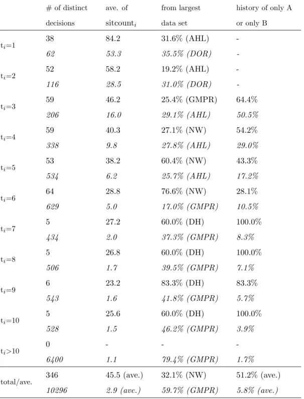
# of distinct decisions ave. of sitcounti from largest data set
history of only A or only B ti=1
38 62 84.2 53.3 31.6% (AHL) 35.5% (DOR) -ti=2
52 116 58.2 28.5 19.2% (AHL) 31.0% (DOR) -ti=3
59 206 46.2 16.0 25.4% (GMPR) 29.1% (AHL) 64.4% 50.5% ti=4
59 338 40.3 9.8 27.1% (NW) 27.8% (AHL) 54.2% 29.0% ti=5
53 534 38.2 6.2 60.4% (NW) 25.7% (AHL) 43.3% 17.2% ti=6
64 629 28.8 5.0 76.6% (NW) 17.0% (GMPR) 28.1% 10.5% ti=7
5 434 27.2 2.0 60.0% (DH) 37.3% (GMPR) 100.0% 8.3% ti=8
5 506 26.8 1.7 60.0% (DH) 39.5% (GMPR) 100.0% 7.1% ti=9
6 543 23.2 1.6 83.3% (DH) 41.8% (GMPR) 83.3% 5.7% ti=10
5 528 25.6 1.5 60.0% (DH) 46.2% (GMPR) 100.0% 3.9% ti>10
0 6400 -1.1 -79.4% (GMPR) -1.7% total/ave. 346 10296 45.5 (ave.) 2.9 (ave.) 32.1% (NW) 59.7% (GMPR) 51.2% (ave.) 5.8% (ave.)
Table 2: Distinct decisions inSe, split up according to player positiont. Note: The …rst entry in each cell describes the restricted data set where sitcounti>10, the second, italicized entry describes the full
data set. Abbreviations: AHL-Alevy/Haigh/List 2006, DOR-Drehmann/Oechssler/Roider 2005, NW-Nöth/Weber 2003, DH-Dominitz/Hung 2004, GMPR-Goeree et al 2007.12
The tables show the large variety of decision situations in the meta data set. For example, the …rst entries in the cells of the second column of Table 2 show that for each of the player position up to t= 6, there are between 38 and 64 distinct decisions among those with sitcounti >10. The
second column of Table 1 shows that these sets of distinct situations comprise several thousand individual decisions at each player position. For player positions 7; :::;10, which appear in only six experiments, there are much fewer suitable decisions available, and not a single decision with t >10 satis…es the requirement that sitcounti >10.
The third columns of the two tables show the strong decrease of sitcounti for increasing player
positions: due to the fact that later positions can have many more di¤erent histories, their average number of identical decisions is much lower. Nevertheless, there are large numbers of identical decisions even in later positions. E.g. for t= 6, each of the 1844 decisions that are included in the restricted data set appears 51.7 times on average. Averaging across all decisions in the restricted data set, decisions appear identically in 196.5 cases each. Table 2 shows that averaging across distinct decisions, each decision appears 45.5 times –this is necessarily lower because the decisions with many identical occurances do no get larger weight in this average.
The fourth columns show the respective largest proportions of observations from an individual data set. Table 1 reveals that in the restricted data set, the experiment by Nöth and Weber (2003), which had many identical games, is rather dominant particularly for player positions t = 5 and t= 6. This is the main reason for not increasing the cuto¤ value for sitcountito a higher value than
10: requiring an even higher number of identical decisions would have increased the precision of mean_payjcontradicti, but it would also have restricted the meta data set even more to its largest
homogeneous subset of decisions. While it is not clear that this or any other kind of selection would introduce problematic biases –because all included experiments are selected situations anyway, and all of them are carefully designed and are equally suitable to detect social learning patterns – it would certainly run counter to the idea of a meta analysis and would reduce the variablility of explanatory variables that are included in the regressions of Section 4.20
2 0
In parallel to the contents of the next sections, robustness checks were run where the cuto¤ was increased to sitcounti >30as well as a separate analysis where the data by Nöth and Weber (2003) were excluded. All linear
The …fth columns of the tables show the proportions of decisions that follow a history where all predecessors agree in their choices. These are potential decisions where social learning should be most prevalent, and they are also relatively simple decisions. The tables show that the selection e¤ect on this variable due to the restriction sitcounti >10is not very strong for player positions up
tot= 6, which make up most of the restricted data set. For player positionst= 1 and t= 2, the variable is not de…ned because there can be no disagreement yet, and for postions 3; :::;6, about half of the decisions follow a history where all previous players agreed.
3
Reluctance to contradict one’s own information
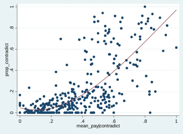
This section shows the main result concerning the question in the title of the paper. Figure 1 plots mean_payjcontradicti against the proportion of contradicting one’s signal among all identical
situations. That is, for each decisions si with sitfreqi > 10, the …gure contains a marker with
x-value mean_payjcontradicti and y-value given by the following variable.
prop_contradicti: Frequency of contradictj = 1across all sj 2Se(si).
Every marker in the scatterplot re‡ects one of the 364 distinct decisions. The regression uses all 15734 individual decisions and not just each distinct situation once, thereby weighting according to sitfreqi. It includes an intercept plus linear, squared and cubed terms of the regressor variable.
The …gure shows a large discrepancy between decisions where mean_payjcontradicti is small
versus large: for the decisions in the left half of the …gure, where the own signal is correct in more than half of the cases, the participants mostly make the correct choice and follow their signal. In contrast, in the decisions depicted in the right half of the …gure the frequency of the signal being correct is smaller than one half but the participants often fail to contradict their signal. Had they made the payo¤-maximizing choice in each case, or even approximately so, the regression line would be an S-shaped line through (0:5;0:5), which is a possible shape of the …tted line with squared and cubed regressors, and it would lie close to 1 in the right half of the …gure. But the proportions in the right half are mostly far away from this optimum. Averaging over all decisions with mean_payjcontradicti 0:5, the frequency of the optimal choice is0:44. In contrast, for the
decisions in left half of the …gure, they make the optimal choice with a frequency of0:91.
0
.2
.4
.6
.8
1
pr
op_cont
radi
ct
0 .2 .4 .6 .8 1
mean_pay|contradict
Figure 1: Proportion of contradicting own signal across all decisions in the restricted data set with sitcounti >10. Note: 346 distinct decisions, 15734 individual decisions in total. Regression
The correspondence at least has the right slope as the proportion of contradicting the signal in-creases in mean_payjcontradicti. A natural question to ask is how large does mean_payjcontradicti
have to be for the average participant to optimally contradict their own signal with more than prob-ability0:5. The answer is most easily seen by observing that the regression line reaches the level of 0:5at mean_payjcontradicti = 0:68. (Considering a series of subsamples of the data, conditioning
on prop_contradicti, would yield the same result.) The empirical likelihood of the own signal being
correct therefore has to be very low before the typical participant discards the signal. On average, only in decisions where the signal is wrong more than twice as often as it is correct (i.e., at an empirical odds ration of 2:1 against the signal) do the participants contradict this signal with a frequency of more than one half.
Without making any assumptions on the process of decisionmaking, one can conclude from these observations that choices cannot be best responses to rational expectations about the underlying distributions. Whatever the true structure of the data generating process, it cannot be that the participants optimally respond to it because otherwise the proportions in the right half of the …gure would lie closer to 1. One can even reject that participants only imperfectly respond to rational expectations but in a way that is unbiased between following and contradicting the own signal. Under such a model, rational expectations would still imply that the unsystematic disturbances would only attenuate the S-shape in the estimated correspondence: for large samples the regression consistently estimates the frequency of contradicting the own signal as a function of this action’s value (consistent for sitcounti! 1). Under rational expectations the turnover point therefore lies
at mean_payjcontradicti= 0:5. But the vertical distance between the regression line and(0:5;0:5)
is highly signi…cant.21 22 Section 4 will provide further tests and a more precise formulation of the 2 1Thet-value for the vertical distance between the regression line and(0:5;0:5)ist= 24:15in a regression where the errors are clustered by groupi.
2 2
A straightforward argument rules out the possibility that the failure of the regression line to go through(0:5;0:5) is driven entirely by random deviations of mean_payjcontradicti from its true expected value. One can estimate
the standard deviation of mean_payjcontradicti for each decisionsi, using the fact that mean_payjcontradicti is a
counting variable with a known sample size. The mean of these estimated standard deviations is 0:05, far smaller than the horizontal distance of the regression line from (0:5;0:5). Another possible check of the potential impact of limited sample sizes is to consider only cases where sitcounti exceeds more stringent thresholds, so that more
rational expectation hypothesis.
But recall the discussion in the introduction, where it was argued that the frequency of making the optimal choice is only a partial indicator of success because the particpants earn more from making the optimal choice in some situations than in others. To calculate the payo¤ of a participant in decision si, let p(contradicti) be her probability of choosing contradicti = 1. Her expected
earnings are
E[ i] =p(contradicti) E[ ijcontradicti = 1] + (1 p(contradicti)) E[ ijcontradicti = 0].
Here, E[ ijcontradicti = 1] is the expected payo¤ from contradicting the signal – which varies
between decisionssi; sj if they are not identical, and cannot be in‡uenced by the particpant’s action.
Due to the fact that one action yields1i¤ the other action yields0, it holds thatE[ ijcontradicti=
0] = 1 E[ ijcontradicti = 1], so the expression can be rewritten as
E[ i] =p(contradicti) (2E[ ijcontradicti= 1] 1) + 1 E[ ijcontradicti = 1]. (1)
Substituting the sample means into this expression – prop_contradicti for p(contradicti) and
mean_payjcontradicti for E[ ijcontradicti = 1] – yields the actual average earnings in decisions
that are identical tosi. Applying this calculation to all decisions where mean_payjcontradicti 0:5
shows that in these situations the participants earn 0:53 of the normalized pie size. In contrast, had they chosenp(contradicti) = 1in all of these decisions, they would have earned0:64, and they
would have earned0:36from doing the opposite, p(contradicti) = 0. Had they simply randomized
between A and B, they would have predicted the correct urn in half of the cases and therefore would have earned 0:5. Hence, their actual earnings are much closer to the payo¤ from simple randomization than they are to the payo¤-maximizing strategy. In contrast, the same calculation for the decisions with mean_payjcontradicti <0:5shows that in these situations the success of the
participants is much higher: when following the own signal is optimal, the participants earn 0:73 out of the 0:75that they could have earned if they had always made the optimal choice.
reliable values of mean_payjcontradicti are used. The pattern is unchanged when such additional restrictions are
But from this analysis one cannot tell whether there is a bias in one class of situations, or the other class, or in both –one can only establish a discrepancy between the two. Evidently, the data pattern suggests that relative to rational expectations, the participants have a general tendency to follow their signal. To the extent that such a bias exists also in the left half of Figure 1, this bias would help the participants to make the optimal choice. In the right half of the …gure, such a bias would be harmful and particpants could earn more if they were to overcome it. But little can be said about where the anomaly occurs.
In the absence of a structural model of behavior, the analysis therefore does not reveal much about the nature of the deviations from rational expectations. The next section will yield some insights on this issue, by looking for additional systematic patterns across di¤erent subsets of the data. It will demonstrate that the participants’ ability to learn from others depends on whether the other players’actions are in contradiction to the own signal and whether the other participants show an unambiguous string of actions.
I also wish to point out clearly that other contributions to the literature have formulated models and other arguments that speak to the evidence presented above. Willinger and Ziegelmeyer (1998) were the …rst to raise the tendency to follow the own signal, which was later discussed most explicitly in Nöth and Weber (2003) and Goeree et al (2007). In the model estimates of Goeree et al (2007), the weight on the own signals is estimated to be signi…cantly higher than the weight of a player’s belief before observing the signal. In the error-rate analyses of Nöth and Weber (2003), Oberhammer and Stiehler (2003), Kübler and Weizsäcker (2004) and Kraemer, Nöth and Weber (2006), related arguments are given in the observations that the participants appear to attribute too low precision to other players. But all of these earlier results rely on much more restrictive assumptions about the decisionmaking process, and none has assessed the economic signi…cance of the deviations from optimal play in much detail. This is further pursued in Section 4.
4
Accounting for losses: Behavioral versus situational
determi-nants of payo¤s
This section investigates co-variates of behavior, with the initial goal of identifying conditions under which social learning is more or less successful, measured by the frequency with which the participants choose the empirically optimal action. The section will then demonstrate that a substantial proportion of the payo¤ variation between these di¤erent conditions can be attributed to behavioral deviations from a rational-expectations benchmark. For this demonstration, the value of the available information will be held constant across di¤erent situations, so that the remaining payo¤ di¤erences can be attributed to changes in the participants’behavior.
The …rst explanatory variable of interest is a proxy for the amount of available information. It describes whether the participants observe more or fewer other participants in the current repetition of the game:
latei: An indicator variable that takes on the value of 1 if the participant has player position
t 5.
One may expect that social learning is more successful in cases where latei = 1 because people
may be more easily pursuaded to pay attention to others if the amount of observable actions is large. On the other hand, they may also …nd it harder to interpret a large set of actions relative to a small set.
The second variable of interest indicates whether or not the actions of other players tend to contradict the player’s own signal.
counter_majorityi: An indicator of whether or not the player’s own signal is in contradiction
to a strict majority of the predecessors’actions. (For example, if predecessors’s actions are AAB and the participant’s signal isb.)
Given that the previous section has already demonstrated a systematic tendendcy towards fol-lowing the own signal, it is natural to suspect that the participants are more successful in situations where other players’actions indicate that they received the same signal (counter_majorityi = 0),
because in these situations the signal tends to be correct.23 2 3
The third co-variate is whether the previous players in the current game unanimously chose the same action.
full_agreementi: An indicator that is 1 if all predecessors chose A or all predecessors chose
B, in the current repetition of the game.
Perfect agreement among predecessors can potentially make learning more successful because the string of observations is easier to interpret. On the other hand, if a player makes the mis-take to follow the own signal too often, then this mismis-take may be more costly in cases with full_agreementi = 1 because in these cases it is more likely that the other players are correct.
Another possibility – which will be con…rmed below – is that full agreement among other players has a especially strong e¤ect on the success of learning when it is interacted with the length of the observed string of actions (latei). Such an interaction e¤ect may arise e.g. due to the di¢ culty of
interpreting long strings of observations that are not unanimous.
The following is the dependent variable of all regressions in this section. It measures whether the participant chooses the action that is empirically optimal.
optimali: An indicator of whether or not the participant chooses the action with higher
em-pirical value. If mean_payjcontradicti >0:5, then optimali is 1 i¤ the participant contradicts her
signal. If mean_payjcontradicti 0:5, optimali is 1 i¤ the participant follows her signal.
The following variable is the empirical value of the optimal action (paralleling the calculation of mean_payjcontradicti):
mean_payjoptimali: The frequency acrosssj 2Seiof receiveing the high payo¤ from choosing
optimali= 1.
The variable mean_payjoptimali is included as a control in some of the subsequent regressions.
Controlling for the value of the actions is relevant because the participants may exhibit a payo¤-sensitive precision of play. For decisions where the empirical value of making the correct choice is low (close to 0:5) the participants may have a relatively low success rate, by either of three mean_payjcontradicti <> 0:5. In the restricted dataset with sitcounti > 10, there are 5146 decision with
counter_majorityi= 1, of which 4012 also have mean_payjcontradicti >0:5. The conceptual di¤erences are that
the value of counter_majorityi is observable to the participants and that it does not rely on estimates of underlying
values, which makes the interpretation of results simpler.
mechanisms: (i) a larger di¢ culty of …nding the optimal action, (ii) a consciously higher likelihood to deviate in situations where less is at stake, (iii) the fact that mean_payjoptimali measures
the "true" underlying expected value with measurement error, so that the optimal action may be misclassi…ed for cases where mean_payjoptimali is close to 0:5. In either case, given that the
dummy variables are correlated with mean_payjoptimali, the latter should be included.
With such a control, the dummy coe¢ cients in the regressions have a distinct interpretation: they describe the size of behavioral changes that are associated with the nature of the situation (as captured by the dummies), but not with the importance of making the respective choices. Under the assumption that the participants have rational expectations about the underlying distributions and best respond to these expectations with equal precision across the dummy categories, all of the dummy coe¢ cients are predicted to approach zero as mean_payjcontradicti approaches the true
expected payo¤. The regressions with controls therefore represent a simple test of the hypothesis that people respond to rational expectations.
The following gives a precise de…nition of the rational-expectations hypothesis that is tested here. Let xi (treatmenti, Ii) be the vector of variables that is observable to the decisionmaker
in situationsi, including the explanatory dummies that are de…ned above. The hypothesis is that
the player uses the relevant payo¤ information that is contained inxi, but disregardsxi otherwise:
a player exhibits (probabilistic) best responses to rational expectations if actionA is chosen i¤
E[ ijA;xi] E[ ijB;xi] + i 0
where i is i.i.d. acrossi, with a distributionF that is symmetric around zero, and independent of
xi. The choice probability is therefore
pi(A) = 1 F(E[ ijA;xi] E[ ijB;xi])
= 1 F(2E[ ijA;xi] 1).
Since the labelling choice of actions A and B is arbitrary in this formulation, one can write the probability of making the empirically optimal choice as1 F(2E[ ijoptimali;xi] 1), which depends
on E[ ijoptimali;xi] alone. Therefore, if a regression controls for E[ ijoptimali;xi] but includes
zero. Since mean_payjoptimali approaches E[ ijoptimali;xi] for large sample sizes (sitcounti !
1), the t-tests for the dummies in a regression with controls for mean_payjoptimali are consistent
tests of rational expectations.
In addition, the following tables will also contain regressions where mean_payjoptimali is not
included. These regressions only contain dummy variables, thus allowing to read o¤ the average success rates for each category from the estimated coe¢ cients.
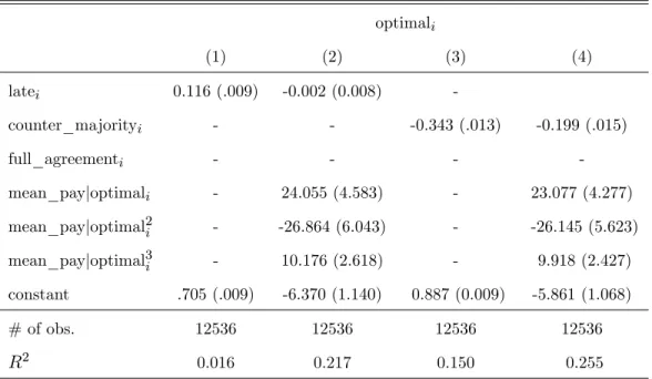
Table 3 considers in columns (1) to (8) the main e¤ects of the above explanatory variables. In all of the subsequent analysis, attention is restricted to player positions t 2, i.e. to those players who observe at least one predecessor in the current repetition of the game.
optimali
(1) (2) (3) (4)
latei 0.116 (.009) -0.002 (0.008)
-counter_majorityi - - -0.343 (.013) -0.199 (.015)
full_agreementi - - -
-mean_payjoptimali - 24.055 (4.583) - 23.077 (4.277)
mean_payjoptimal2i - -26.864 (6.043) - -26.145 (5.623)
mean_payjoptimal3i - 10.176 (2.618) - 9.918 (2.427)
constant .705 (.009) -6.370 (1.140) 0.887 (0.009) -5.861 (1.068)
# of obs. 12536 12536 12536 12536
R2 0.016 0.217 0.150 0.255
Table 3: Frequencies of making the empirically optimal choice. Note: Data includes cases with sitcounti>10 andt 2. Robust standard errors
in parentheses, clustered by groupi.
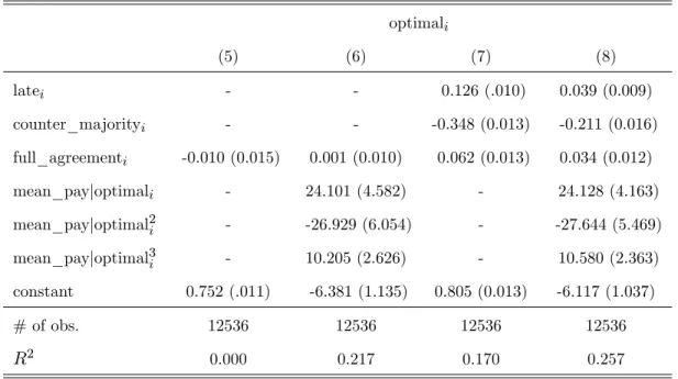
optimali
(5) (6) (7) (8)
latei - - 0.126 (.010) 0.039 (0.009)
counter_majorityi - - -0.348 (0.013) -0.211 (0.016)
full_agreementi -0.010 (0.015) 0.001 (0.010) 0.062 (0.013) 0.034 (0.012)
mean_payjoptimali - 24.101 (4.582) - 24.128 (4.163)
mean_payjoptimal2i - -26.929 (6.054) - -27.644 (5.469)
mean_payjoptimal3i - 10.205 (2.626) - 10.580 (2.363)
constant 0.752 (.011) -6.381 (1.135) 0.805 (0.013) -6.117 (1.037)
# of obs. 12536 12536 12536 12536
R2 0.000 0.217 0.170 0.257
Table 3 (ctd.): Frequencies of making the empirically optimal choice.
optimali
latei=0 latei=1
(9) (10) (11) (12)
full_agreementi -0.048 (0.021) -0.024 (0.013) 0.119 (0.014) 0.080 (0.013)
mean_payjoptimali - 26.689 (6.444) 1.345 (5.398)
mean_payjoptimal2i - -28.364 (8.485) -1.372 (7.054)
mean_payjoptimal3i - 10.039 (3.671) 0.839 (3.024)
constant 0.740 (0.017) -7.382 (1.602) 0.764 (0.010) 0.157 (1.352)
# of obs. 8131 8131 4405 4405
R2 0.002 0.285 0.024 0.084
optimali
latei=0 latei=1
(13) (14) (15) (16)
counter_majorityi -0.246 (0.032) -0.052 (0.032) -0.176 (0.021) -0.158 (.023)
full_agreementi 0.109 (0.020) 0.067 (0.016) 0.146 (0.011) 0.102 (0.011)
(counter_majorityi
full_agreementi)
-0.221 (0.034) -0.178 (0.030) -0.075 (0.032) -0.035 (0.030)
mean_payjoptimali - 27.603 (5.700) 5.423 (5.269)
mean_payjoptimal2i - -31.046 (7.480) -5.943 (6.878)
mean_payjoptimal3i - 11.614 (3.232) 2.325 (2.937)
constant 0.804 (0.018) -7.244 (1.426) 0.835 (0.012) -0.867 (1.315)
# of obs. 8131 8131 4405 4405
R2 0.208 0.315 0.010 0.126
Table 3 (ctd.): Frequencies of making the empirically optimal choice.
The overriding feature of the regressions is the strongly negative e¤ect of counter_majorityi.
In situations where most previous players choose a di¤erent action than is indicated by a partic-ipant’s signal, her frequency of making the empirically optimal choice is much lower. The dif-ference in frequencies is 0:343, relative to an average success rate of 0:887 in the situations with counter_majorityi = 0, see column (3). The result corresponds to the tendency described in Section
3: people far too often follow their own signals, and this is harmful in situations where the majority of previous choices indicates that the signal is likely wrong. In part, the result can be explained by the di¤erent incentives that the participants face depending on the value counter_majorityi. As
column (4) shows, controlling for the incentives by including mean_payjoptimali reduces the size
of the coe¢ cient on counter_majorityi. This re‡ects the fact that mean_payjoptimali is lower in
situations where counter_majorityi= 1, and that participants make the empirically optimal choice
more often when it is important. But even when mean_payjoptimali is controlled for, the partial
e¤ect of counter_majorityi is 0:199, a large and highly signi…cant deviation from the hypothesis
of best responding to rational expectations.
The variable latei has a positive coe¢ cient in column (1), indicating that participants in
posi-tionst 5 have a higher success rate on average, by 11.6 percentage points. However, controlling for mean_payjopti in column (2) shows that the higher success is entirely associated with the
higher incentive to make the optimal choice. Holding mean_payjopti constant, the success rates
are virtually identical between earlier and later positions in the game. Higher earnings for later players are therefore associated with the higher lucrativity of situations. The rate of optimal play improves for later players in the game, but only in correspondence with the higher incentives.
The variable full_agreementi is not correlated with success rates, unless the other dummy
variables are introduced as well (columns (5) to (8)).24 This is surprising because one would have expected learning to be easier when full_agreementi = 1. But the di¤erence between the results
in columns (5) and (6) versus (7) and (8) points at a potential interaction between the dummy variables, which is examined next. Columns (9) to (16) interact the three variables of interest, by separating the data according to lateiand, in columns (13) to (16), by including an interaction term
for (counter_majorityi full_agreementi). The regressions show that a full agreement among the
previous players can indeed strongly increase the success rate, but especially for late positions in the game. This is most directly seen in columns (9) to (12), where full_agreementi has a signi…cant
and positive e¤ect only in the subsample with latei= 1.
The interaction e¤ect of latei and full_agreement is further clari…ed if it is also interacted with
2 4The results on full_agreement are not all robust to excluding subsamples. When restricting the sample tot 3 instead of t 2, there is a small but signi…cant e¤ect of full_agreementi: the dummy coe¢ cient in regression (5)
changes to 0.050 (std. err. 0.014). But in column (7), the analogous coe¢ cient is 0.001 (0.010). When excluding the largest individual data set, Nöth and Weber (2003), full_agreementiis signi…cantly and strongly positively correlated
with optimali, with dummy coe¢ cients of 0.160 (0.038) and 0.20 (0.038) in the regressions corresponding to columns
(5) and (7), and 0.120 (0.039) and 0.176 (0.085) in columns (9) and (11). However, when mean_payjoptimali is
controlled for, parallel to the regressions in columns (6), (8), (10) and (12), the coe¢ cients are reduced to 0.053 (0.032), 0.111 (0.035), 0.050 (0.033) and -0.006 (0.076), respectively. All other results of Tables 3 are qualitatively unchanged when the data are restricted to subsets that excludet= 2situations or the data from Nöth and Weber (2003), or to observations with sitcounti > 30. All conclusions from Table 3 are also supported by repeating the
counter_majorityi, in columns (13) to (16). First consider the case that counter_majorityi = 0.
For these cases, the coe¢ cients of full_agreementi show that observing an unanimous set of actions
increases the success rate by0:109for latei = 0and by0:146for latei= 1. This con…rms the results
of columns (9) to (12) to a somewhat weaker degree, for those situations where the majority of previous actions and the participants’s own signal are in agreement. But for counter_majorityi = 1
and latei = 0, the participants in situations with full_agreementi = 1 have a lower success rate
than with full_agreementi = 0, by a di¤erence of 0:109 0:221 = 0:112.25 For latei = 1, on
the other hand, the participants in situations with full_agreementi= 1 have a success rate that is
higher by 0:146 0:075 = 0:071, as one would expect.
In sum, the discussion shows that for later players, the positive e¤ect of having previous players who all agree is larger than for early players. The e¤ect counteracts to a substantial degree the negative e¤ect of counter_majorityi: in situations where all three dummy variables are 1 (e.g.
histories with informationAAAAborAAAAAb), the average success rate is0:730, which is higher than in any other constellation with counter_majorityi = 1. In other words, the participants are
fairly successful in learning from others only when the evidence conveyed by the others’choices is strong (latei= 1) and unambiguous (full_ageementi = 1).
Controlling for the empirical value of the optimal action (in regression in even-numbered columns) does not qualitatively change these conclusions but only reduces the size of the e¤ects somewhat. This shows again that the hypothesis of best responding to rational expectations is violated –the participants exhibit systematically lower success rates in those situations where the actions of others are not unambiguous.
As an illustration, Figure 2 contains the same variables as Figure 1, plotting the empirical value of contradicting one’s signal against the corresponding frequency, but highlights with solid markers
2 5
In part, this is driven by the observation that players at positionst= 2andt= 3have a very low success rate if counter_majority= 1 (0:404and 0:453, respectively) and that by de…nition of the variables, in these cases it is always true that full_agreementi= 1holds because there cannot be a strict but ambiguous majority with only one
or two predecessors. But it also re‡cets that there is no positive e¤ect of full_agreementieven for players att= 4:
conditional on counter_majorityi = 1 andti = 4, the frequency of optimali is 0:558for full_agreementi = 0 and
0:564for full_agreementi= 1.
0
.2
.4
.6
.8
1
pr
op_cont
radi
ct
0 .2 .4 .6 .8 1
mean_pay|contradict
Figure 2: Proportion of contradicting own signal. Note: See Figure 1. Highlighted situations are those with latei = 1 and fullagreehisi = 1:
the set of situations with latei = 1and full_agreementi = 1. The solid line is the regression line of
this subsample, whereas the dashed line is for the remaining subsample. As the …gure shows, the rate of contradicting the own signal when it is optimal are much higher if the history of previous choices is long and unanimous. These situations are the typical cascade situations, where Bayes Nash Equilibrium predicts that players disregard their signals. The fact that the success rates are much lower in the remainder of the situations was never emphasized in the previous literature, to my knowledge. Instead, the high success rates along paths where cascades would theoretically arise was often pointed out (see e.g. Anderson and Holt, 1997, Kübler and Weizsäcker, 2005).
The remainder of the section describes the payo¤s of participants in the di¤erent classes of situations that are captured by the dummy variables, and discusses the relative e¤ect of behavioral
versus situational in‡uences on the payo¤ variance. I will restrict attention to the two identi…ed signi…cant e¤ects of counter_majorityi (columns (3), (4) of Table 3) and of full_agreementi for
later player positions (columns (11), (12)). The relevant distinction between the two former classes of situations will be adressed in Table 4, and the latter in Table 5.
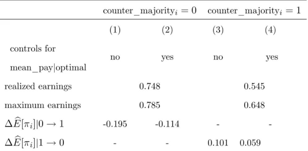
The …rst step is to calculate the obtained payo¤s for the di¤erent classes of situations. Parallel to expression (1) one can calculate the average realized payo¤ in all situations that are identical to si as
mean( i) =mean(optimali) (2 mean_payjoptimali 1) + 1 mean_payjoptimali. (2)
The row labelled "realized earnings" in Table 4 shows the corresponding values (averages of mean( i)across all situations) for each of the categories of counter_majority. Across all situations
with counter_majorityi = 0, the participants receive an average payo¤ of0:748, and they receive
an average payo¤ of0:545if counter_majorityi = 1.
Had they always chosen the empirically optimal action, how much would they have earned? This can be calculated by replacing optimali by 1 in expression (2). The row labelled
"maxi-mum earnings" shows the corresponding calcualtion results. Comparing realized with maxi"maxi-mum earnings, it shows that for counter_majorityi = 1, the realized earnings are much further from
their maximum than for counter_majorityi = 0. But the entries also show that situations with
counter_majorityi = 1 are much more lucrative: choosing the optimal action yields 0:785 on
average, compared to 0:648 in situations with counter_majorityi = 1. Overall, the calculations
illustrate that the di¤erence in the realized earnings is driven by both the di¤erence in behavior and the di¤erence in incentives. Both components have a substantial impact.
To explore this further, one can ask the following counterfactual question: by how much would the di¤erence in the earnings decrease if the di¤erence in behavior was absent? For example, how much would earnings under counter_majorityi = 1 increase if the participants were equally
suc-cessful in making optimal choices as under counter_majorityi = 0? The answer can be generated
by replacing mean(optimali) in expression (2) by(mean(optimali) dummy coef f icient), where
the dummy coe¢ cient is taken from the regressions of column (3) or (4) of Table 3. This coef-…cient measures the di¤erence in the success rates, so that subtracting it generates the desired
counterfactual behavioral change. The di¤erence to the realized payo¤s is then given by
b
E[ i]j1!0 = dummy coef f icient (2 mean_payjoptimali 1),
which is reported in the last row of Table 4. Similarly, the term Eb[ i]j0 ! 1 in the
preced-ing row measures the counterfactual change in payo¤s under counter_majorityi = 0 that would
arise if behavior was equally (un)successful as in situations with counter_majorityi = 1. For each
of the two rows, the …rst entry measures the counterfactual payo¤ increase when using only the simple dummy regression of column (3) of Table 3 – hence uses the simple di¤erence in the data average as the dummy coe¢ cient – whereas the second entry uses the regression that controls for mean_payjoptimali when describing the behavioral di¤erence (column (4)). Recall that
un-der the hypothesis that participants best respond to rational expectations, the inclusion of such controls should capture any impact of the nature of the situation, including the dummy values. Hence, the counterfactual payo¤ changes in Table 4’s columns (2) and (4) are estimates of the payo¤ changes that are associated with the observed deviations from rational expectations. For example, the entries in column (4) of Table (4) show that if behavior was equally successful under counter_majorityi = 1 as it is under counter_majorityi= 0, payo¤s under counter_majorityi = 1
would increase by almost 6 percentage points, to about 0:61. The observed payo¤ di¤erences between the two classes of situations would be substantially reduced if behavior was identical.
Table 5 repeats the above exercises for the distinction between situations where full_agreementi =
1 versus full_agreementi = 0, both conditional on latei = 1. Here, too, it shows that the sizable
di¤erences in realized payo¤s between the two classes of situations (0:759versus 0:663) would be substantially reduced –to at most half of the actual di¤erence –if behavior was equally successful in both categories. This con…rms that also for this second "irrational" reaction to the nature of situations, the payo¤ was strongly a¤ected.
counter_majorityi = 0 counter_majorityi = 1
(1) (2) (3) (4)
controls for
mean_payjoptimal
no yes no yes
realized earnings 0.748 0.545
maximum earnings 0.785 0.648
b
E[ i]j0!1 -0.195 -0.114 -
-b
E[ i]j1!0 - - 0.101 0.059
Table 4: Payo¤ results in response to behavioral variations depending on counter_majorityi
full_agreementi= 0
latei= 1
full_agreementi = 1
latei = 1
(1) (2) (3) (4)
controls for
mean_payjoptimal
no yes no yes
realized earnings 0.663 0.759
maximum earnings 0.758 0.813
b
E[ i]j0!1 0.061 0.041 -
-b
E[ i]j1!0 - - -0.074 -0.050
Table 5: Payo¤ results in response to behavioral variations depending on full_agreementi
5
Conclusions
The paper presents a large meta dataset from thirteen cascade game experiments, and applies a simple counting technique to infer that the success rate is low in decisions where it would be optimal to follow the choices of others. This demonstrates a violation of rational expectations about the conditional likelihoods of the states of the world. This conclusion can be drawn without imposing any structural model of what players might believe about the behavior of the players that acted before her.
The paper also discusses the payo¤ impact that the deviations from rational expectations have. In situations where the own signal runs counter to a strict majority of previous choices, the partic-ipants earn much less than in the remaining situations, and it is estimated that the "behavioral" deviations from rational expectations account for a large share of the payo¤ di¤erence. If the par-ticipants were as successful in identifying the optimal choice in these decisions as they are in the remaining decisions, the payo¤ di¤erence would be reduced by a proportion between one quarter and one half. A similar result occurs for cases where the previous players were not in full agreement, which causes players to mis-read the available information and forgo substantial payo¤s.
The methodology of the test for rational expectations in Section 4 is simple but novel in experi-mental economics, so the question arises whether it can be applied to other experiexperi-mental (or other) data sets. It surely can, and in fact aspects of it are already applied in numerous studies: it is often calculated –though not often enough –how much the participants in an experiment give up due to their failure to choose a best response against the empirical distribution of payo¤-relevant random variables. The innovative component of the methodology here is to not only estimate the empirical value of the available actions, but to also use it as an explanatory variable in regressions that describe behavior. This yields a test of rational expectations that does not rely on a structural behavioral model.26 The key requirement is to have su¢ cient data so that the empirical value of an action is a useful estimate of the underlying "true" expectation. With a meta data set, which typically has lots of data, one can apply this approach to a large variety of decisions. As in other 2 6See Weizsäcker (2003) and Goeree and Holt (2004) for Quantal–Response-Equilibrium-based tests of rational expectations in normal form games.
meta analyses, the wealth of data thus allows multiple di¤erent perspectives on the data –includ-ing some that are unanticipated by the original studies’ authors – without giv–includ-ing up statistical reliability. This general advantage of meta analyses is probably underrated, too, in the literature.27
References
Alevy, Jonathan E., Michael S. Haigh and John A. List (2007). "Information cascades: Evidence from a …eld experiment with …nancial market professionals." Journal of Fi-nance 62, 151-180.
Anderson, Lisa R. (2001). "Payo¤ E¤ects in Information Cascade Experiments." Eco-nomic Inquiry 39, 609-614.
Anderson, Lisa R., and Charles A. Holt (1997). "Information Cascades in the Labora-tory." American Economic Review 87, 847-862.
Bikhchandani, Sushil, David Hirshleifer, and Ivo Welch (1992). "A Theory of Fads, Fashion, Custom, and Cultural Change as Informational Cascades." Journal of Political Economy 100, 992-1026.
Celen, Bogachan, and Shachar Kariv, Distinguishing Informational Cascades From Herd Behavior in the Laboratory." American Economic Review 94, 484-497.
Choi, Syngjoo, Douglas Gale, and Shachar Kariv (2004). "Learning in Networks: An Experimental Study." Working Paper, New York University.
Cipriani, Marco, and Antonio Guarino (2005). "Herd Behavior in a Laboratory Finan-cial Market." American Economic Review 95, 1427-1443.
Dominitz, Je¤, and Angela A. Hung (2004). "Homogeneous Actions and Heterogeneous 2 7Harless and Camerer (1994), Zelmer (2003), Oosterbeek, Sloof and van de Kuilen (2004), Huck, Normann and Oechssler (2004) and Engel (2007) are earlier examples of meta analyses in experimental economics that tackle novel questions.