On the Compilation of Programs into their Equivalent Constraint
Representation
Franz Wotawa and Mihai Nica
Technische Universität Graz, Institute for Software Technology, Inffeldgasse 16b/2, 8010 Graz, Austria E-mail: {wotawa,mihai.nica}@ist.tugraz.at
Keywords:constraint satisfaction problems, hyper-graph decomposition, debugging
Received:March 15, 2008
In this paper we introduce the basic methodology for analyzing and debugging programs. We first convert programs into their loop-free equivalents and from this into the static single assignment form. From the static single assignment form we derive a corresponding constraint satisfaction problem. The constraint representation can be directly used for debugging. From the corresponding hyper-tree representation of the constraint satisfaction problem we compute the hyper-tree width which characterizes the complexity of finding a solution for the constraint satisfaction problem. Since constraint satisfaction can be effectively used for diagnosis the conversion can be used for debugging and the obtained hyper-tree width is an indi-cator of the debugging complexity.
Povzetek: ˇClanek opisuje analiziranje programov in iskanje napak v njih.
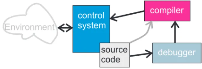
Figure 1: Interaction between the control and the debug-ging system
1 Introduction
Ideally intelligent systems should provide self-reasoning and reflection capabilities in order to react on internal faults as well as on unexpected interaction with their environ-ment. Reflection capabilities are highly recommended for systems with strong robustness constraints, like space ex-ploration probes or even mobile robots. A scenario, for example, is a robot that although having a broken engine, should reach a certain position. Without self-reasoning or reflection such a robot would simple fail to reach its goal. Another example would be a robot where the software fails because of a bug. In this situation a robot should recover and ideally repair itself. Note that even exhaustive testing does not prevent a program from containing bugs which might cause an unexpected behavior in certain situations.
In this paper we do not focus on whole systems which comprise hardware and software. Instead we are discussing how to represent programs to allow for reflection which can be used for enhancing the system with debugging func-tionality. In the context of this paper debugging is defined as fault localization given a certain test-case. We do not
take care of verification and test-case generation which is used for fault detection and repair. In order to compute the fault location we follow the model-based diagnosis ap-proach (22) but do not rely on logical models but use con-straints instead for representing programs. The obtained constraint representation can be directly used for comput-ing diagnosis, e.g., by uscomput-ing specialized diagnosis algo-rithms like the one described in (12; 25; 26).
Although, reflection and debugging capabilities are a desired functionality of a system they provoke additional computational complexity which can hardly be handled by the system directly because of lack of computational power. Note that model-based diagnosis is NP complete. Hence, a distributed architecture would be required which separates the running control program from the debugging capabili-ties. In Figure 1 we depict the proposed architecture. The debugging module takes the source code of the original sys-tem which is in this case a control syssys-tem and a test-case to localize and repair the fault. The changed source code is compiled and transferred back to the original system.
In the proposed architecture there are several open is-sues which have to be solved. The first is regarding the test case. In particular one is interest in the origin of the test case. One way would be to have a monitoring system which checks the internal state of the control system. In case of a faulty behavior, the given inputs coming from the sensors, the internal state and the computed output together with the information regarding the expected output is used as a test case. The second issue is related to fault localization and repair. There is literature explaining fault localization and repair which can be used, e.g., (13; 24; 17; 23).
mis-behavior. This does not necessarily directly lead to good repair suggestions. Repair definitely requires knowledge about further specification details and incorporating differ-ent test-cases should help a lot. A detailed discussion of repair is outside the scope of this paper and still an impor-tant topic of research. The third and last issue is a more technical one. After recompiling the new program has to replace the old one on the fly which might cause additional problems because of ensuring integrity and consistency of the system’s behavior.
Making systems self-aware and giving those self-healing capabilities increases their autonomy, which is important in missions like space exploration where the system can-not be directly controlled for whatever reason. The paper contributes to this research in providing a methodology for fault localization in programs. The methodology requires the availability of the source code and test cases. It com-piles the program into their equivalent constraint represen-tation and uses a failure-revealing test case to compute di-agnosis candidates.
The paper is organized as follows. We first introduce the basic ideas behind our approach by means of an ex-ample. Afterwards, we go through all necessary steps of the conversion process, which finally leads to the constraint representation of programs. This section is followed by a presentation of experimental results we obtained from our implementation. The experiments focus on structural prop-erties of the programs’ constraint representation because the structural properties have an impact on the complex-ity of debugging. Finally, we discuss related research and conclude the paper.
2 Diagnosis/debugging
In this section we motivate the idea behind our approach by means of an example program that is expected to com-pute the area and circumference of a circle from a given diameter.
1. r = d/2;
2. c = r*pi;
3. a = r*r*pi;
Obviously the statement in line 2 is faulty. A possible repair would be c = 2*r*pi; or c = d*pi;. We know this because of our knowledge in mathematics. How-ever, in the more general case where large programs are involved, we have to rely on a process in order to detect, localize, and correct a fault. Such a process deals with the question: ‘How can we find out what’s wrong in the program’ and is a standard in today’s software engineering processes. In software engineering we first have to detect the fault. This is done in practice using test-cases or proper-ties together with formal verification methods. In our case we rely on test cases. One test case which allow to detect the faulty behavior would be settingdto 2 and requiringc
to be2πandato beπ. The program computes the valueπ for both variablescandawhich contradicts the test case.
This contradiction can be used to locate the fault. One way would be to have a look at the first definition of vari-able cwhich has assigned a wrong value and trace back using the dependencies between variables. In this caseris defined in line 1 and used in line 2. Hence, line 1 and 2 are possible fault candidates. This approach uses only struc-tural information coded in the program and might overes-timate the number of diagnosis candidates. Another ap-proach would be to assume some line of the program to be faulty. In this case the statement corresponding to the line does not provide any known functionality. For example, when assuming line 2 to be faulty, we do not know how to compute a value for c. Therefore, we do not get any contradicting information and the assumption is consistent with the given test-case. Unfortunately, this is also the case when assuming line 1 to be faulty and only considering the computation of values like specified in the semantics of the programming language, i.e., from the begin of the program to its end.
The situation changes when considering the statement as equations where no direction of information flow is given. An equation liker = d/2is a constraint which specifies a relationship betweenrandd. When we now assume the constraint corresponding to line 1 to be faulty we can com-pute a value forrusing the given test-case. From the con-straint corresponding to line 3 a = r2π anda = π we
derive r = 1and finally usingc = rπ leads toc = π which contradicts the given expected value forcwhich is 2π. Hence, the assumption in this case contradicts the ob-servations and cannot be a single-fault candidate. Only line 2 remains as single fault. The reason for this improvement is that when using constraints we have the capabilities for reasoning backwards.
Summarizing the above discussion, a solution to the de-bugging problem would be to convert programs into their constraint representation and use it for debugging. We choose a constraint representation because equations as well as logical sentences can be represented and integrated, and because of the availability of tools. However, there are still some challenges we have to solve.
First, variables might be defined more than once in a program. Every definition has to be considered separately. Programs comprise conditional and loop statements. How to handle them? For the first problem and the conditionals we propose the use of the static single assignment (SSA) form of programs which is used in compiler construction.
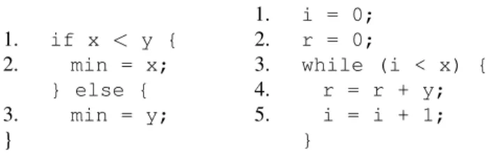
con-1. if x < y {
2. min = x; } else {
3. min = y;
}
Figure 2: A program com-puting the minimum of two numbers
1. i = 0;
2. r = 0;
3. while (i < x) {
4. r = r + y;
5. i = i + 1; }
Figure 3: A program for computing the product of two natural numbers
ditionals. A similar technique can be applied to solve the recursive procedure calls challenge.
Finally, we have to handle arrays and other programming language constructs like pointers or objects. In this paper, we present an approach for handling arrays. The other as-pects of programming languages are ignored. This is due to the fact that our main application area is the embedded-systems domain. Programs used in embedded-embedded-systems usu-ally are restricted and do not use of features like dynamic memory allocation because such features are error prone and likely lead to problems during operation.
3 Conversion
In this section, we describe the conversion process of pro-grams into their equivalent CSP representation in detail. For more information regarding CSPs we refer the reader to Dechter (11). We start with converting programs into their loop-free equivalents which are used as basis for the conversion into the SSA form. Finally, we show how to extract the CSP from the SSA form. The complexity of the proposed compilation approach is composed of the com-plexity of each conversion step. While SSA construction and CSP extraction can be both handled in polynomial time computing a loop-free equivalent depends on the number of necessary iterations. This number depends on the pro-gram’s complexity. In this section we use the programs given in Figure 2 and 3 as running examples. We further assume without restricting generality of the approach that the programs to be converted have a Java like syntax (ig-noring object-oriented elements).
3.1 Loop-free programs
When executing while-statements they behave like a con-ditional statement in one step. If the condition is fulfilled the statements in the block are executed and the while-statement is executed again afterwards. Otherwise, the while-statement is not executed. Hence, it is semantically correct to represent while-statements using an infinite num-ber of nested if-statements, i.e.,while ( C ) { B }
is equivalent to
if ( C ) {
B if ( C ) {
B if ( C ) {
B if ... } } }
Crepresents the condition, andB the statements in the sub-block of the while statement.
Of course it is not possible in practice to compile while-statements into an infinite number of conditionals. In-stead we assume that the number of iterations of the while-statement never exceeds a certain limit sayn. We argue that faults can be detected using test-cases which cause a small number of iteration and that it is therefore – for the pur-pose of debugging – not necessary to consider larger val-ues ofn. Moreover, we might introduce a procedure which is called whenever the limit is reached. This information would give us back additional information which we might use for increasingnin a further step. To set a small bound for the number of iterations is also used in a different con-text. Jackson (18) uses a similar idea which he calledsmall scope hypothesisin his Alloy system for verification.
We formalize the bounded conversion from while-statements into nested if-while-statements by introducing the function Γ : P L×N 7→ P L whereP L represents the programming language.
Γ(while ( C ) { B}, n) =
=
if (C) {BΓ(while (C) {B}, n−1)} ifn >0
if (C) { too_many_iterations; } otherwise
Considering the above discussion it is obvious that the following theorem which states the equivalence of the pro-gram and its loop-free variant with respect to their behavior has to hold.
Theorem 3.1. Given a programΠ∈P Lwritten in a pro-gramming languageP Land a numbern∈N. Πbehaves equivalent to Γ(Π, n) for an input I iff the execution of
Γ(Π, n)onIdoes not reachtoo_many_iterations.
We now use the program from Figure 3 and n = 2to show the application ofΓwhich leads to the following pro-gram:
1. i = 0;
2. r = 0;
3. if (i < x) {
4. r = r + y;
5. i = i + 1;
6. if (i < x) {
7. r = r + y;
8. i = i + 1;
9. if (i < x) {
10. too_many_iterations; } } }
complexity of a program which is corresponds to the num-ber of iterations depending on the size of the inputs is now represented by the size of the converted program. Hence, we easily can give an estimate for the size of the converted programs (and also the number of iterations) when limiting the size of the input.
3.2 Static single assignment form
The SSA form is an intermediate representation of a pro-gram, which has the property that no two left-side vari-ables share the same name, i.e., each left-side variable has a unique name. Because of this reason the SSA form is of great importance when building the CSP. Since all variables are only defined once the SSA form allows for a clear repre-sentation of the dependencies that are established between different variables inside the corresponding program. The SSA representation of a program is sometime also an in-termediate step in the compiling process; basically before compiling a java file, first a transformation is undertaken and the SSA form is obtained. The obtained form will be the form used as input for the compiler.
In order to compile loop-free programs into SSA we have to analyze the program and rename all variables such that each variable is only defined once without changing the behavior of the program. Basically, this compilation is done by adding an unique index to every variable, which is defined in a statement. Every use of this variable in the succeeding statement is indexed using the same value. This is done until a new definition of the same variable occur.
For example, the following program fragment on the up-per side can be converted into its SSA representation bel-low.
1. x = a + b;
2. x = x - c;
The SSA representation:
1. x_1 = a_0 + b_0;
2. x_2 = x_1 - c_0;
Although, converting programs comprising only assign-ment stateassign-ments is easy, it is more difficult for programs with loop or conditional statements. In our case we only need to consider conditional statements. The idea behind the conversion of conditional statement is as follows: The value of the condition is stored in a new unique variable. The if- and the else-block are converted separately. In both cases the conversion starts using the indices of the variables already computed. Both conversions deliver back new in-dices of variables. In order to get a value for a variable we have to select the last definition of a variable from the if-and else-part depending on the condition. This selection is done using a functionΦ. Hence, for every variable which is defined in the if- or the else-branch we have to introduce a selecting assignment statement which calls theΦfunction. For example, corresponding SSA form of the program fragment
if (C) { .. x = .. } else {
.. x = .. }
is given as follows:
var_C = C; .. x_i = .. .. x_j = ..
x_k = Φ(x_i,x_j,var_C);
The function Φ is defined as follows: Φ(x, y, b) =
½
x ifb y otherwise
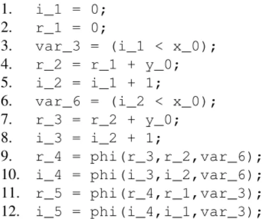
For algorithms for computing the SSA form and more information regarding theΦfunction we refer the reader to (9; 7; 27). The SSA representation for the programs from Figure 2 and 3 are depicted in Figure 4 and 5 respec-tively. Note that we represent theΦfunction as a function callphiin the program. It is possible to write a function body forphithat exactly represents the behavior of theΦ function. Hence, the program and its SSA representation can be executed on the same input even at the level of the programming language.
It is easy to see that the SSA form of a program always behaves equivalent to the original program, which we state in the following theorem.
Theorem 3.2. Given a programΠ ∈ P L. The SSA rep-resentationΠ0 ∈ P LofΠis equivalent toΠwith respect to the semantics ofP L, i.e., for all inputsIboth programs return the same output.
For debugging purposes the input output equivalence, which is similar to the input output conformance (IOCO) used in testing, is sufficient. The SSA representation allows us to map, with little effort, the diagnosis set of programΠ0
to the original equivalent programΠ.
In the following subsection we describe how arrays and function calls can be handled. Afterwards we discuss the compilation of programs into constraint systems.
3.3 Extensions
In the previously described conversion process we still face two important challenges as they are the conversion of ar-rays and procedure calls. In this section, we tackle both challenges and present conversion rules that have to be ap-plied before converting the resulting source code in a SSA form.
1. var_1 = ( x_0 < y_0 );
2. min_1 = x_0;
3. min_2 = y_0;
4. min_3 = phi(min_1,min_2,var_1);
Figure 4: The SSA form of the program from Fig. 2
1. i_1 = 0;
2. r_1 = 0;
3. var_3 = (i_1 < x_0);
4. r_2 = r_1 + y_0;
5. i_2 = i_1 + 1;
6. var_6 = (i_2 < x_0);
7. r_3 = r_2 + y_0;
8. i_3 = i_2 + 1;
9. r_4 = phi(r_3,r_2,var_6);
10. i_4 = phi(i_3,i_2,var_6);
11. r_5 = phi(r_4,r_1,var_3);
12. i_5 = phi(i_4,i_1,var_3);
Figure 5: The SSA form of the loop-free variant of the pro-gram from Fig. 3
Given an array A of length n > 0 with elements ha1...ai...ani. The access to elements is assumed to be
done using the [] operator, which maps from A and a given indexito the array elementai. For example,z = A[1]gives you back the first element of arrayA. So far, arrays seem not to be very difficult to handle in our conver-sion process. If reaching a statement z = A[1]during SSA conversionAhas only be represented asA_k where kis the currently given unique indexkforA. But how to handle statements likeA[m] = A[n] + 3? In this case, obviously Ahas to be assigned a new index, but how to handle the following program fragment?
. . .
A[1] = 2; A[2] = 4;
. . .
A SSA translation into
. . .
A_1[1] = 2; A_2[2] = 4;
. . .
would be wrong because this transformation does not respect previously done array changes in the appropriate manner. In order to respect the underlying semantics, we have a closer look at it. Assume a program fragmentA[i] = f(~x)where thei-th element ofAis set to the outcome of function f given parameters ~x. This statement only changes thei-th element but not the others. Formally, we define the semantics as follows:
{A}// A before the statement A[i] = f(~x)
{A’}// A after the statement
with A’[i] = f(~x) and ∀j ∈ {1, . . . , n}, i 6= j: A’[j] = A[j]. As a consequence, we introduce a func-tionΨthat implements this semantics and replace the orig-inal statement with A = Ψ(A,i,f(~x)). The function
Ψ is similar toΦand can be implemented such that the converted program is equivalent to the original one with respect to its semantics.
For example, consider the following program fragment: 1. A[1] = 5;
2. A[2] = A[1] + 5;
Accordingly to our conversion rule we obtain the new fragment:
1. A = psi(A,1,5);
2. A = psi(A,2,A[1] + 5);
The SSA representation is not based on the new fragment and captures the semantic in the appropriate way.
1. A_1 = psi(A_0,1,5);
2. A_2 = psi(A_1,2,A_1[1] + 5);
Note thatΨorpsican be implemented as a function in order to ensure the equivalent behavior even in the context of program execution. Assume that psi has the formal argumentsA,i,eand that the length of an array can be ac-cessed via a functionlength, then the body of the function is given as follows:
j = 1;
while (j < length(A)) { if (j==i) {
B[j] = e; } else {
B[j] = A[j]; }
j = j + 1; }
return B;
written in the same programming language. A proce-dure callM(a1, . . . , an)with actual parametersa1, . . . , an causes the execution ofM’s body where the formal parame-ters are assigned to their corresponding actual parameparame-ters, i.e., xi = ai. Hence, a transformation is easy. We only have to assign values to the formal parameter, which can be done using assignments, and use the body of the proce-dure instead of the proceproce-dure call.
In cases where the procedure returns a value, we have to introduce a new variableM_return. We further replace
return ewithM_return = e, and finally, we intro-duce a new assignment, whereM_returnis used appro-priately. The described transformation of the return state-ment is only correct, whenever a procedure has only one of those statements. This is not a restriction because we al-ways can modify a program to fulfill this requirement. For simplicity, we also assume that the variables used in bod-ies of procedures and the one used in the main program are different except in cases of global variables.
We now explain the idea behind the conversion using an example program where a procedurefoois called
. . .
x = foo(2,y,z-1);
. . .
Now assume that foo has three formal parameters
x1,x2,x3and the following body:
v = x1 + x2; v = v - x3; return v;
When applying the described conversion rule, we obtain the following program fragment:
x1 = 2; x2 = y; x3 = z-1; v = x1 + x2; v = v - x3; foo_return = v; x = foo_return;
This program can be easily compiled into its SSA form:
x1_1 = 2; x2_1 = y_0; x3_1 = z_0-1; v_1 = x1_1 + x2_1; v_2 = v_1 - x3; foo_return_1 = v_2; x_1 = foo_return_1;
We now extend the above idea to the general case, where we might face recursive procedure calls. The idea behind the conversion is the same, but similar to the handling of iterations of a while statement, we have to set a bound on the maximum number of recursive replacements dur-ing conversion. For this purpose we assume that there is
such a boundM Cgiven for a procedureMin a calling con-text. Similar to while statements we introduce a function ˆ
Γ :P L×N7→ P Lthat defines the bounded compilation of a not necessarily recursive procedure call:
ˆ
Γ([x = ]M( a1,...,an ), i) =
=
x1 = a1;...xn = an; ˆ
Γ(δ0(M), i−1)
[x = M_return; ] ifi≤M C
too_many_recursions; otherwise
Note that δ0 denotes the body of method M, where
the return statement return e has been changed to
M_return = e. Moreover,Γˆ is assumed to be defined for all other statements where the statement itself is re-turned without any changes. Hence, when applying Γˆ to the body of a method, all statements are examined and left as they are with the exception of a new method call. With these additional assumptions the compilation function can be generally applied.
We illustrate the conversion using a program only com-prising the callx = foo(1,2);where the body offoo
is given as follows:
r = 0;
if (x1 > 0) { r= foo(x1-1,x2); r = r + x2;
}
return r;
The following program represents the recursion-free variant of the program callingfoowith 1 allowed iteration, which is sufficient for specific procedure callfoo(1,2)
in order to return the correct result.
x1 = 1; x2 = 2;
// 1. recursive call
r = 0;
if (x1 > 0) { x1 = x1 - 1; x2 = x2;
// 2. recursive call
r = 0;
if (x1 > 0) {
too_many_iterations; }
M_return = r;
// returning from 2. call
r = M_return; r = r + x2; M_return = r;
// returning from 1. call
x = M_return;
3.4 Constraint representation
Constraint satisfaction problems (CSPs) have been intro-duced and used in Artificial Intelligence as a general knowledge representation paradigm of knowledge. A CSP (V, D, CO)is characterized by a set of variablesV, each variable having a domainD, and a set of constraintsCO which define a relation between variables. The variables in a relationr∈COare called the scope of the relation. An assignment of values fromDto variables fromV is called an instantiation. An instantiation is a solution for a CSP, iff it violates no constraint. A constraint is said to be vi-olated by an instantiation, if the value assignment of the variables in the scope of the constraint are not represented in the relation of the constraint. There are many algorithms available for computing valid instantiations, i.e., solutions for a CSP. A straight-forward algorithm is backtrack search where variable values are assigned and consistency checks are performed until a valid solution is found. Moreover, it is well known that CSPs can be solved in polynomial time under some circumstances, i.e., the CSP must be acyclic, which we discuss later. Yannakakis (30) proposed such an algorithm. Based on this algorithm there are diagnosis al-gorithms (12; 25) available, which can be used for debug-ging directly providing there is a CSP representation for programs. For more information and details on CSPs we refer the reader to DechterŠs book (11).
The last step in the conversion process is to map pro-grams in SSA form to their CSP representation. This ex-traction of the constraints from the statements of the SSA representation can be easily done. The algorithm is pretty straight forward and only implies analyzing the SSA repre-sentation line by line. In this conversion step, each line of the SSA representation is mapped directly to a constraint. Hence, all variables of a statement map directly to the scope of the constraint. The constraint relation is given by the statement itself by interpreting the assignment operator as an equivalence operator. For example, the statementx_2 = x_1 + 2is mapped to a constraint having 2 variables
x_2andx_1and where the relation is stated as an equa-tion of the form x_2 =x_1+ 2. Note that the latter rep-resentations is a more flexible one because it can also be read, for example, as x_2−x_1= 2.
The CSP representation of the program from Figure 2 is given as follows:
Variables: V =
½
{var_1, x_0, y_0, min_1, min_2, min_3}
¾
Domains: D={D(x) =N|x∈V}
Constraints: CO=
var_1 = (x_0< y_0), min_1 =x_0, min_2 =y_0, min_3 =phi(min_1,
min_2, var_1)
When comparing the CSP representation of the program with its SSA form, which is depicted in Figure 4, we see that both representations are very close to each other. It is
easy to prove that the SSA form of a program is equivalent to its CSP representation with respect to the behavior.
Theorem 3.3. Given a programΠ, its SSA representation
Π0, the corresponding CSPC
Π. The value assignments of
the variables inΠ0, which are caused by executingΠ0 on an inputIare a solution to the corresponding CSPCΠand
vice versa.
From this theorem and the others we conclude that the transformation is behavior neutral and in this way the CSP representation captures the behavior of the program. As a consequence, the CSP representation can be directly used for debugging. As already mentioned there are circum-stances under which the algorithm is more effectively and there are situations where the computation of solutions is hard. This holds now directly for debugging and we are in-terested in classifying programs regarding their debugging complexity. We define debugging complexity as a measure that corresponds to the complexity of computing a solution using CSP algorithms. In the following, we discuss struc-tural properties of CSPs, which can be used for classifica-tion and which are based on the hyper-graph representaclassifica-tion of programs.
In the hyper-graph representation of a CSP the variables of the CSP represent vertices, and the constraint scopes the hyper-edges. Thus hyper-edges connect possible more than one vertex. Hyper-graphs can be used to classify CSPs re-garding their complexity of computing a solution. As al-ready mentioned, solutions for CSPs with corresponding acyclic hyper-graphs can be computed in polynomial time (see (30)). Such hyper-graphs can be directly represented as hyper-trees. Unfortunately, not all CSPs are acyclic. But the good story is that cyclic CSPs can be converted into an equivalent CSP that is acyclic. What is needed is to join the right constraints. Joining constraints, however, is a draw-back because it is time and space consuming. In the worst case all constraints have to be joined in order to finally re-ceive the acyclic equivalent CSP representation, which is of course intractable.
As a consequence, one only gains computational advan-tages from the conversion of hyper-graphs into hyper-trees if the number of constraints to be joined is as minimal as possible. This number is referred to as hyper-tree width. More information regarding hyper-graphs and hyper-tree composition which allows to convert hyper-graphs into hyper-trees can be found in (14; 15). The hyper-graph and its corresponding hyper-tree for the CSP introduced above is depicted in Figure 6. The hyper-tree width for this exam-ple is 2.
Figure 6: Hyper-graph (left) and corresponding hyper-tree (right) for the SSA form given in Fig. 4
therefore on the hyper-tree width of programs.
4 Experimental results on the
hyper-tree width
As explained in the previous section the hyper-tree width has an impact on the complexity of debugging when using constraints a means for intermediate representation formal-ism. Gaining knowledge about the hyper-tree width of pro-grams is therefore of importance. In this respect this sec-tion reports on the hyper-tree width of several programs. For this purpose, we implemented the conversion proce-dure in Java and used a constraint system that was imple-mented at out institute. For the hyper-tree decomposition we used an implementation provided by the TU Wien (see (16)). In particular, we made use of the Bucket Elimina-tion algorithm based decomposiElimina-tion which is explained in (29). All experiments were carried out on a PC (Pentium 4, 3 GHz, 1 GB Ram).
The experiments are based on small programs that vary from 40 to 400 lines of code. The lines of code of the cor-responding SSA forms and the size of constraint system in terms of number of constraints and variables are higher due to used while statement and their transformation to condi-tional statements. In particular, we wanted to give an em-pirical answer to the following research questions.
– Thorup (28) stated that there is limit of 6 for the hyper-tree width of structured programs. The theorem is based on using control dependence information and does not consider data dependences. Because the lat-ter is of importance for debugging and our compila-tion respects those dependences, we wanted to know whether given limit still applies.
– The compilation of while statements and recursive procedure calls leads to an increase of statements and to a nested if-then-else structure. The question is how the nesting depth, i.e., the number of iterations for unrolling the while statements or recursive proce-dure calls, influences the hyper-tree width? Moreover, one might be interested whether there is a maximum bound on the hyper-tree with in such cases.
The environment for carrying out the empirical study is not the optimal for answering the above research question but the best one can expect today. The reason ist that the
ID LOC #W #I It HW T
1 70 1 6 3 5 1 s
1 70 1 6 50 5 364 s
2 110 0 11 - 5 1 s
3 70 4 5 3 5 11 s
3 70 4 5 20 6 2040 s
4 80 0 0 - 4 1 s
5 70 0 0 - 4 1 s
6 70 0 0 - 2 1 s
7 400 0 0 - 9 7 s
8 400 2 0 3 50 1000 s
8b 400 2 0 3 12 122 s
9 400 1 0 5 16 120 s
9 400 1 0 10 27 621 s
9 400 1 0 20 54 3959 s
9 400 1 0 35 51 16450 s
9 400 1 0 50 55 19245 s
10 400 1 0 10 20 80 s
10 400 1 0 20 23 274 s
10 400 1 0 50 25 2400 s
10 400 1 0 60 29 4120 s
10 400 1 0 70 25 4770 s
11 400 0 0 - 10 8 s
12 400 1 0 3 15 120 s
12 400 1 0 6 27 2580 s
12 400 1 0 10 43 3415 s
13 400 1 0 15 53 4010 s
14 60 0 0 - 2 1 s
15 50 1 4 3 6 1 s
15 50 1 4 10 6 5 s
15 50 1 4 100 6 456 s
16 40 7 0 1 2 1 s
16 40 7 0 10 3 600 s
Figure 7: Evolution of the hyper-tree width for different complexity programs
Bucket Elimination based decomposition algorithm is only an approximation algorithm and thus the solutions needs not to be minimal once. However, because of the size of the corresponding constraint systems other algorithms are hardly of use because they would take too much time and space.
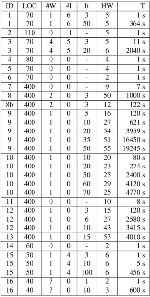
The finally obtained results for the programs are de-picted in Figure 7. There the programs are given a num-ber (ID). The lines of codes (LOC) of the original program, the number of while statements (#W), the number of if-statements (#I), the number of iterations used to unroll the while-statements (I), the hyper-tree width (HW) obtained, and the time (T) required to compute the hyper-tree width are given.
1. x = 10;
2. y = 20;
3. while (x<100){
4. x = x + y;
5. y = y + 2;
Figure 8: Small example programtest
the hyper-tree width ranges from 9 to 55. Even in the case where there is no unrolling of while statements (programs 7 and 11) the hyper-tree width ranges from 9 to 10. All of these programs represent digital circuits including some variants (like 8 and 8a) with a complex data flow.
Based on the obtained empirical results, we have to re-tract Thorup’s theorem (28) because there are many pro-grams that result in a constraint system of a larger hyper-tree width than 6. Note that it is not very likely to find a hyper-tree decomposition with a smaller width for the given programs. Moreover, the approximation algorithm seems to produce approximations, which are close to the optimum.
The second research question is harder to answer. In all experiments, we observed that after a certain number of it-erations the hyper-tree width remains almost the same. For example take a look at program 9 and 10. In both cases it seems that the hyper-tree width reaches an upper bound. Of course because of the used approximation algorithm there is a variance in the obtained width. But it seems to be al-ways around a certain value. More experiments have to be carried out in order to justify these findings.
For the purpose of motivating why the hyper-tree width stays constant after a certain number of considered iter-ations of the while statement, we use a small program
test, which is given in Figure 8. For test we know that the maximum hyper-tree width is 3. This upper bound is reached after 2 times unrolling of the while statement, i.e., replacements of the while statement with nested if-statements.
In our example, we now compute the SSA form and the corresponding constraint systems for programtestusing 3 nested if-statements. The resulting SSA form and the constraint system are depicted in Figure 9 and Figure 10 respectively.
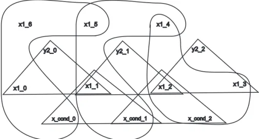
The hyper-graph corresponding to the constraint repre-sentation oftestis given in Figure 11. Note that for the sake of clarity the graphical representation only comprises the constraints from the while structure in which the vari-ablexis involved. From the hyper-graph it can be easily seen that the edges follow a certain pattern, which is re-peated in every unrolling of the while statements. Hence, there is a possibility that the hyper-graph decomposition can be applied to these subparts of the hyper-graph sepa-rately and combined afterwards, which might lead to a con-stant hyper-tree width after a certain amount of unrolling steps.
In summary, we obtained the following results from the
experimental study:
– The hyper-tree width of programs might become very large. Usually problems of hyper-tree width of 5 to 10 depending on the application domain are considered hard problems.
– In case of unrolling while-statements or recursive calls; it seems that the hyper-tree width reaches an upper bound. This would be an indication that debug-ging does not necessarily become more difficult, when the number of iterations increases. Note that the num-ber of unrolling steps of while statements does depend on the considered test case, which is an independent criteria.
– The time for computing the hyper-tree width can be very large, which might be unacceptable in some cir-cumstances. This can be for example the case when interactive debugging is a requirement. For automated debugging or off-line debugging the time for conver-sions is not a limiting factor. However, decreasing the overall analysis time is an open challenge.
What remains of interests is the question, why a certain program has a larger hyper-tree width than another simi-lar program? Obviously the data and control dependences influence the overall hyper-tree width. But in case of sim-ilar programs the differences regarding the dependencies might not be large enough to justify high differences of the obtained hyper-tree width. This holds especially in case where a program comprises while statements. In the next section, we focus on this aspect and discuss one cause that leads to such an observation.
5 Discussion
In the performed experiments we observe that programs, which have a high hyper-tree width and where the number of iterations necessary to reach the maximum hyper-tree width is large, have less data dependences in the sub-block of the while statement. We illustrate these findings by means of two example programssum1andsum2, which are depicted in Figure 12 and Figure 13 respectively. Both programs have about the same structure. In both programs a variableiis increased in every iteration until it reaches 100. Moreover, the hyper-tree width of both programs is about the same (2 and 1 forsum1andsum2respectively) when the number of considered unrolling steps is 1.
However, the situation changes, when considering more nested if-statements as a replacement for the while state-ment. For sum1 the maximum hyper-tree width of 4 is reached after 3 iterations. Forsum2the maximum hyper-tree width of 8 is reached after 12 unrolling steps. If con-sidering the difference between the minimum and the max-imum hyper-tree width, we obtain another different out-come. For sum1 the difference is only 1, whereas for
1. x1_0 = 10;
2. y2_0 = 20;
3. cond_0=x1_0<100;
4. x1_1=x1_0+y2_0;
5. y2_1=y2_0+2;
6. cond_1=cond_0&&x1_1<100;
7. x1_2=x1_1+y2_1;
8. y2_2=y2_1+2;
9. cond_2=cond_1&&x1_2<100;
10. x1_3=x1_2+y2_2;
11. y2_3=y2_2+2;
12. x1_4=phi(x1_2,x1_3,cond_2);
13. y2_4=phi(y2_2,y2_3,cond_2);
14. x1_5=phi(x1_1,x1_4,cond_1);
15. y2_5=phi(y2_1,y2_4,cond_1);
16. x1_6=phi(x1_0,x1_5,cond_0);
17. y2_6=phi(y2_0,y2_5,cond_0);
Figure 9: The SSA form of programtest(Fig. 8)
1. (x1_0 ),
2. (y2_0 ),
3. (X_cond_0 , x1_0 ),
4. (x1_1 , x1_0 , y2_0 ),
5. (y2_1 , y2_0 ),
6. (X_cond_1 , X_cond_0 , x1_1 ),
7. (x1_2 , x1_1 , y2_1 ),
8. (y2_2 , y2_1 ),
9. (X_cond_2 , X_cond_1 , x1_2 ),
10. (x1_3 , x1_2 , y2_2 ),
11. (y2_3 , y2_2 ),
12. (x1_4 , x1_2 , x1_3 , X_cond_2 ),
13. (y2_4 , y2_2 , y2_3 , X_cond_2 ),
14. (x1_5 , x1_1 , x1_4 , X_cond_1 ),
15. (y2_5 , y2_1 , y2_4 , X_cond_1 ),
16. (x1_6 , x1_0 , x1_5 , X_cond_0 ),
17. (y2_6 , y2_0 , y2_5 , X_cond_0 ).
Figure 10: The constraints fortest(Fig. 8)
x1_6 x1_5 x1_4
x1_0
y2_1
x1_1 x1_2 x1_3
x_cond_1
x_cond_0 x_cond_2
y2_2 y2_0
Figure 11: The hyper-graph of the constraint system from Fig. 10
1. a = f + i;
2. b = g + h;
3. while (i < 100) {
4. x = x + a + b;
5. i = x + i + 1;
6. }
Figure 12: Programsum1
1. a = f + i;
2. b = g + h;
3. while (i < 100) {
4. x = a + b;
5. i = i + 1;
6. y = c + d;
7. }
By having a closer look at the programs we detect a ma-jor difference in their structure, which might explain this high difference in the hyper-tree width. For the variable
xthat is used in the block of programsum1a new value is computed in each iteration of the while statement. The outcome of variablexdepends on the number of iterations and therefore on variablei(and the condition of the while statement). This is not the case for variablexand variable
yin programsum2. Both variables are assigned the same value in each iteration step. For performance reason such assignment statements should be always placed outside a loop. In case of programsum2the values of variables in an iteration not necessarily depends on the previous iteration but on a variables that have been computed before calling the while statement. It seems that this difference makes the structure of the hyper-graph more complex, which leads fi-nally to a higher hyper-tree width.
The given example shows that hyper-tree width may in-dicate an unwanted program structure. In programsum2
either there are variables missing at the right side of state-ments 4 and 6, or both statestate-ments should be given outside the while statement because of performance reasons. Obvi-ously, such problems can be detected using some rules like the following:
If a variablevis defined in the sub-block of a while state-ment, then there should be at least one not necessarily dif-ferent statement in the same block that usesv.
Hyper-tree width offers another way for detecting such problematic cases occurring in programs.
6 Related research
Collavizza and Ruehner (8) discussed the conversion of programs into constraint systems and their use in software verification. Their work is very close to ours. The conver-sion steps are about the same and they also use the SSA form as an intermediate representation from which con-straints can be obtained. However, there are some impor-tant differences. In their work the focus is on verification and not on debugging. They do not explain how to handle arrays and procedure calls as we did in the paper. More-over, the structural analysis of programs using the concept of tree-decomposition methods and in particular hyper-tree decomposition is new. This holds also for the findings de-rived from the empirical analysis, which are of importance for automated debugging.
The authors of (31) proposed to diagnose errors in pro-grams using constraint programming. Their approach re-quires that the programmer provides contracts, i.e., pre-and post-conditions, for every function. However, the au-thors do not investigate the complexity of solving the re-sulting problem and the scalability to larger programs. In particular, they do not consider structural decomposition or other methods which could make the approach feasible. Moreover, the practical applicability of their approach is also limited because it requires that contracts are specified
for every function, which is very often not the case in real-world programs. Furthermore, their work does not properly handle recursive function calls.
Various authors, e.g., (13; 24; 20; 21), have described models to be used for fault localization using model-based diagnosis. Almost all of the work makes assumptions re-garding the program’s structure, uses abstractions which lead to the computation of too many diagnosis candidates, or does not handle all possible behaviors at once. The latter models, for example, consider one execution trace which prevent the diagnosis engine of remove some diagnosis candidates. In our representation we consider all possible behaviors up to a given boundary. This should lead to a re-duction of the number of diagnosis candidates. In (19) Köb and Wotawa discussed the use of Hoare logic for model-based debugging which requires a Hoare logic calculus for computing diagnosis. Although, we share the same ideas on automated debugging, the described approach, which comprises the conversion to CSPs and their direct use, is new. From our point of view the described approach gen-eralizes previous research directions.
Other work on debugging include (4; 5; 6). All of them are mainly based on program slicing (10). (6) integrates slicing and algorithmic program debugging (2) and (5) does the same for slicing and delta debugging (1). Critical slic-ing (4) which is an extension of dynamic slicslic-ing that avoids some of the pitfalls, can also be used in debugging. Be-cause of the nature of slicing and the other techniques these approaches require more or less user interaction and cannot be used for really automated debugging. More information regarding other approaches to debugging and a good clas-sification of debugging system is provided in (3).
7 Conclusion
In this paper we introduced a methodology for compil-ing programs into their equivalent CSP representation. The methodology comprises the conversion of while state-ment into their equivalent nested if-statestate-ment representa-tion from which the SSA form is generated. From the SSA form itself we finally obtain the CSP representation. In the paper we argued that the CSP representation can be effec-tively used for debugging and allows for computing a com-plexity metrics for debugging, i.e., the hyper-tree width. This is due the fact that the complexity of debugging based on CSPs depends on the hyper-tree width. For the purpose of debugging we assume the existence of the source code and test cases, which reveal the fault. Another advantage of the CSP representation is that the available algorithms for constraint solving and in particular diagnosis can be di-rectly used.
shows that debugging itself is a complex task. From the empirical analysis we also obtain that previous work, which was mainly based on control dependences, on an upper bound of 6 for the hyper-tree width of programs cannot be justified in case of debugging in general. For a specific program there might be an upper bound even when compil-ing while statements in their equivalent nested if-statement representation.
Future research includes to solve the upper bound prob-lem in the general case and to apply the debugging ap-proach to smaller and medium size programs. The inte-gration of the CSP representation and given program asser-tions like pre- and post-condiasser-tions is also of interest.
Acknowledgement
This work has been supported by the FIT-IT research project Self Properties in Autonomous Systems project (SEPIAS) which is funded by the Austrian Federal Min-istry of Transport, Innovation and Technology and the FFG and by the Austrian Science Fund (FWF) within the project "Model-based Diagnosis and Reconfiguration in Mobile Autonomous Systems (MoDReMAS)" under grant P20199-N15. Moreover, we want to thank Nysret Musliu for providing us with an implementation of the hyper-graph decomposition.
References
[1] Andreas Zeller and Ralf Hildebrandt. Simplifying and isolating failure-inducing input. IEEE Transac-tions on Software Engineering, 28(2), feb 2002.
[2] Ehud Shapiro. Algorithmic Program Debugging. MIT Press, 1983.
[3] Nahid Shahmehri, Mariam Kamkar, and Peter Fritz-son. Usability criteria for automated debugging sys-tems.J. Systems Software, 31:55–70, 1995.
[4] Richard A. DeMillo, Hsin Pan, and Eugene H. Spaf-ford. Critical slicing for software fault localization. InInternational Symposium on Software Testing and Analysis (ISSTA), pages 121–134, 1996.
[5] Neelam Gupta, Haifeng He, Xiangyu Zhang, and Ra-jiv Gupta. Locating faulty code using failure-inducing chops. In Automated Software Engineering (ASE), pages 263–272, November 2005.
[6] Mariam Kamkar. Application of program slicing in algorithmic debugging. Information and Software Technology, 40:637–645, 1998.
[7] Marc M. Brandis and H. Mössenböck. Single-pass generation of static assignment form for structured languages.ACM TOPLAS, 16(6):1684–1698, 1994.
[8] H. Collavizza and M. Rueher. Exploration of the ca-pabilities of constraint programming for software ver-ification. InTools and Algorithms for the Construc-tion and Analysis of Systems (TACAS), pages 182– 196, Vienna, Austria, 2006.
[9] Ron Cytron, Jeanne Ferrante, Barry K. Rosen, Mark N. Wegman, and F. Kenneth Zadeck. Efficiently computing static single assignment form and the con-trol dependence graph. ACM TOPLAS, 13(4):451– 490, 1991.
[10] Mark Weiser. Programmers use slices when debug-ging. Communications of the ACM, 25(7):446–452, July 1982.
[11] Rina Dechter. Constraint Processing. Morgan Kauf-mann, 2003.
[12] Yousri El Fattah and Rina Dechter. Diagnosing tree-decomposable circuits. In Proceedings 14th
Inter-national Joint Conf. on Artificial Intelligence, pages 1742 – 1748, 1995.
[13] Gerhard Friedrich, Markus Stumptner, and Franz Wotawa. Model-based diagnosis of hardware designs. Artificial Intelligence, 111(2):3–39, July 1999.
[14] Georg Gottlob, Nicola Leone, and Francesco Scar-cello. On Tractable Queries and Constraints. In Proc. 12th International Conference on Database and Expert Systems Applications DEXA 2001, Florence, Italy, 1999.
[15] G. Gottlob, N. Leone, and F. Scarcello. A comparison of structural CSP decomposition methods. Artificial Intelligence, 124(2):243–282, 2000.
[16] http://www.dbai.tuwien.ac.at/proj/hypertree/ in-dex.html
[17] A. Griesmayer, R. Bloem, and B. Cook. Repair of boolean programs with an application to C. In Proc. 18th Conference on Computer Aided Verifica-tion (CAV’06), pages 358–371, Seattle, Washington, USA, August 2006.
[18] Daniel Jackson. Software abstractions: logic, lan-guage, and analysis. MIT Press, 2006.
[19] Daniel Köb and Franz Wotawa. Fundamentals of debugging using a resolution calculus. In Luciano Baresi and Reiko Heckel, editors,Fundamental Ap-proaches to Software Engineering (FASE’06), volume 3922 of Lecture Notes in Computer Science, pages 278–292, Vienna, Austria, March 2006. Springer.
[21] Wolfgang Mayer, Markus Stumptner, Dominik Wieland, and Franz Wotawa. Can ai help to improve debugging substantially? debugging experiences with value-based models. InProceedings of the European Conference on Artificial Intelligence, pages 417–421, Lyon, France, 2002.
[22] Raymond Reiter. A theory of diagnosis from first principles.Artificial Intelligence, 32(1):57–95, 1987.
[23] S. Staber, B. Jobstmann, and R. Bloem. Finding and fixing faults. InProc. 13th Conference on Correct Hardware Design and Verification Methods, pages 35–49. Springer-Verlag, 2005. LNCS 3725.
[24] Markus Stumptner and Franz Wotawa. Debugging Functional Programs. In Proceedings 16th
Inter-national Joint Conf. on Artificial Intelligence, pages 1074–1079, Stockholm, Sweden, August 1999.
[25] Markus Stumptner and Franz Wotawa. Diagnos-ing tree-structured systems. Artificial Intelligence, 127(1):1–29, 2001.
[26] M. Stumptner and F. Wotawa. Coupling CSP decom-position methods and diagnosis algorithms for tree-structured systems. InProc. 18thInternational Joint
Conf. on Artificial Intelligence, pages 388–393, Aca-pulco, Mexico, 2003.
[27] M.N. Wegman and F.K. Zadek. Constant propaga-tion with condipropaga-tional branches.ACM Transactions on Programming Languages and Systems, 13(2), April 1991.
[28] Mikkel Thorup.All Structured Programs have Small Tree-Width and Good Register Alloca-tion,Information and Computation Journal, Volume 142,Number 2,Pages 159-181,1998.
[29] Artan Dermaku, Tobias Ganzow, Georg Gottlob, Ben McMahan, Nysret Musliu, Marko Samer. Heuristic Methods for hypertree Decompositions, DBAI-TR-2005-53, Technische Universität Wien, 2005.
[30] M. Yannakakis. Algorithms for acyclic database schemes. In C. Zaniolo and C. Delobel, editors, Proceedings of the International Conference on Very Large Data Bases (VLDB-81), pages 82–94, Cannes, France, 1981.