*Correspondence to Author:
S.E. Fadugba
Department of Mathematics, Ekiti State University, Ado Ekiti, Nigeria
How to cite this article:
S.E. Fadugba and T. E. Olaose-bikan. Comparative Study of a
Class of One-Step Methods for the Numerical Solution of Some Initial Value Problems in Ordinary Differ-ential Equations. Research Journal of Mathematics and Computer
Sci-ence, 2018; 2:9 .
eSciPub LLC, Houston, TX USA. Website: http://escipub.com/
Research Journal of Mathematics and Computer Science
(ISSN:2576-3989)
Research Article RJMCS (2018) 2:9
Comparative Study of a Class of One-Step Methods for the
Numerical Solution of Some Initial Value Problems in Ordinary
Differential Equations
We emphasized explicitly on the derivation and implementation of a new one-step numerical method for the solution of initial value problems in ordinary differential equations. In this paper, we aimed at comparing the newly developed method with oth-er existing methods such as Euloth-er’s method, Trapezoidal rule and Simpson’s rule. Using these methods to solve some initial value problems of first order ordinary differential equations, we discovered that the results compared favorably, which led to the conclusion that the newly derived one-step numerical method is approximately correct and can be used for any related first order ordinary differential equations.
Keywords: Numerical solution, One-step method, Ordinary dif-ferential equation.
1 S.E. Fadugba and 2T. E. Olaosebikan
1,2 Department of Mathematics, Ekiti State University, Ado Ekiti, Nigeria
ABSTRACT
http://escipub.com/research-journal-of-mathematics-and-computer-science/ 2 1. INTRODUCTION
Various numerical methods have been developed for the solution of some initial value problems of ordinary differential equations. Some of the Numerical Analysts who have worked extensively on the development of numerical methods are: Fatunla, (1976), Lambert (1991), Ibijola, (1997 and 1998), Kama and Ibijola (2000), Butcher (2003), Zarina et al. (2005), Aboiyar et al. (2015), Fadugba and Falodun (2017), just to mention a few. The efficiency of all these contributed efforts from these Numerical Analysts in numerical analysis had been measured and tested for their stability, accuracy, convergence and consistency properties. The accuracy properties of different methods are usually compared by considering the order of convergence as well as the truncation error coefficients of the various methods. Research has shown that for a method to be suitable for solving any sets of initial value problems in ordinary differential equations, it must have all the mentioned characteristics. In this paper, we compare a new one-step numerical method with existing methods with the above mentioned characteristics in mind to solve some initial value problems in ordinary differential equations of the form:
𝑦′= 𝑓(𝑥, 𝑦); 𝑦(𝑎) = 𝜂, −∞ < 𝑦 < ∞, 𝑎 ≤ 𝑥 ≤ 𝑏 (1)
in the interval (𝑥𝑛, 𝑥𝑛+1) by interpolating function given by
𝐹(𝑥) = 𝑎0+ 𝑎1𝑒−𝛼𝑥
(2)
where 𝑎0 and 𝑎1 are real undetermined coefficients.
The rest of the paper is organized as follows. Section Two consists of some basic properties. Section Three is the development of the new scheme. Section Four consists of the numerical example, discussion of results and concluding remarks.
2. SOME BASIC PROPERTIES
We consider the following basic properties namely; stability, consistency and convergence.
(a) Stability: A numerical method is said to be stable if the difference between the numerical solution and the exact solution can be made as small as possible, that is if there exists two positive constant e0 and Ksuch that the following holds;
0
( )
n n
y y x K e
(3)
(b) Consistency: A numerical method with an increment function (x y hn, n, )is said to be consistent with the initial value problem under consideration if
(x y hn, n, ) f x y( n, n)
(4)
(c) Convergence: A numerical method is said to be convergent if for all initial value problem satisfying the hypothesis of Lipschitz condition given by
2 1 2 1
( , ) ( , )
f x y f x y L y y
(5)
where the Lipschitz constant is denoted by L.
Remark 1: The necessary and sufficient conditions for convergence are stability and consistency.
3. DEVELOPMENT OF A NEW ONE STEP NUMERICAL METHOD
Suppose we have the initial value problem of the form:
𝑦′ = 𝑓(𝑥, 𝑦); 𝑦(𝑥0) = 𝑦0
(6) Let us assume that the theoretical solution 𝑦(𝑥) to (6) can be locally represented in the interval (𝑥𝑛, 𝑥𝑛+1), 𝑛 ≥ 0 by the interpolating
polynomial function: 𝐹(𝑥) = 𝑎0+ 𝑎1𝑒−𝛼𝑥
(7)
where 𝑎0, and 𝑎1 are real undetermined coefficients.
We also assume that 𝑦𝑛 is a numerical estimate
http://escipub.com/research-journal-of-mathematics-and-computer-science/ 3 𝑓𝑛 = 𝑓(𝑥𝑛, 𝑦𝑛). We define mesh points as
follows:
𝑥𝑛 = 𝑎 + 𝑛ℎ, 𝑛 = 0, 1, 2, … or 𝑥𝑛+1 = 𝑎 + (𝑛 + 1)ℎ, 𝑛 = 1, 2, …
Therefore, from (7), we obtain the following derivatives
𝐹1(𝑥) = −𝛼𝑎
1𝑒−𝛼𝑥
(8)
𝐹2(𝑥) = 𝛼2𝑎
1𝑒−𝛼𝑥
(9)
From (7), we have that 𝑎0 = 𝐹(𝑥) − 𝑎1𝑒−𝛼𝑥
(10)
Also from (8), we obtain
𝑎1 = − 𝐹1(𝑥) 𝛼𝑒−𝛼𝑥
(12)
Putting (12) into (9), yields
𝐹2(𝑥) = −𝛼𝐹1(𝑥)
(13)
Similarly, from (12) and (10), we have:
𝑎0 = 𝐹(𝑥) − 𝐹1(𝑥)
𝛼
(14)
Now, imposing the following constraints on the interpolating function (7) in the following order:
a. The interpolating function (7) must coincide with the theoretical solution at 𝑥 = 𝑥𝑛 and 𝑥 = 𝑥𝑛+1 such that:
𝐹(𝑥𝑛) = 𝑎0+ 𝑎1𝑒−𝛼𝑥𝑛
𝐹(𝑥𝑛+1) = 𝑎0 + 𝑎1𝑒−𝛼𝑥𝑛+1
b. The derivative of 𝐹1(𝑥), 𝐹2(𝑥) and 𝐹𝑛(𝑥)
coincide with 𝑓(𝑥), 𝑓1(𝑥) and 𝑓𝑛−1(𝑥)
respectively. That is; 𝐹1(𝑥) = 𝑓𝑛
𝐹2(𝑥) = 𝑓𝑛1
From conditions (a) and (b) above, it follows that:
𝐹(𝑥𝑛+1) − 𝐹(𝑥𝑛) ≡ 𝑦𝑛+1− 𝑦𝑛 Therefore, we have:
𝑎0+ 𝑎1𝑒−𝛼𝑥𝑛+1− (𝑎0+ 𝑎1𝑒−𝛼𝑥𝑛) = 𝑦𝑛+1− 𝑦𝑛
Re-arranging terms yield:
𝑦𝑛+1 = 𝑦𝑛+ 𝑎1(𝑒−𝛼𝑥𝑛+1 − 𝑒−𝛼𝑥𝑛)
(15)
From the mesh points, we have 𝑥𝑛 = 𝑎 + 𝑛ℎ
or
𝑥𝑛+1 = 𝑎 + (𝑛 + 1)ℎ
From (15), the term (𝑒−𝛼𝑥𝑛+1 − 𝑒−𝛼𝑥𝑛) can be written as
𝑒−𝛼𝑥𝑛+1− 𝑒−𝛼𝑥𝑛 = 𝑒−𝛼(𝑎+(𝑛+1)ℎ) − 𝑒−𝛼(𝑎+𝑛ℎ) by factorization and setting 𝑎 = 0, we have:
𝑒−𝛼(𝑎+(𝑛+1)ℎ) − 𝑒−𝛼(𝑎+𝑛ℎ) = 𝑒−𝛼𝑛ℎ(𝑒−𝛼ℎ − 1)
(16)
Putting (12) and (16) in (15), we have the new scheme follow:
𝑦𝑛+1 = 𝑦𝑛−𝑓𝑛
𝛼 (𝑒
−𝛼ℎ − 1)
(17)
Using power series expansion to fourth term and by factorization, (17) becomes:
𝑦𝑛+1 = 𝑦𝑛− ℎ (−1 +𝛼ℎ
2! − 𝛼2ℎ2
3! ) 𝑓𝑛
(18)
Equation (18) is the proposed one-step method.
3.1 Properties of the Scheme
3.1.1 Convergence of the Scheme
We establish the numerical integration algorithm for which (18) can be expressed as one-step method in the form:
𝑦𝑛+1 = 𝑥𝑛+ ℎ∅(𝑥𝑛, 𝑦𝑛; ℎ)
(19)
where ∅(𝑥𝑛, 𝑦𝑛; ℎ) is the increment function. We proceed to derive the increment function for our scheme from:
𝐹(𝑥) = 𝑎0+ 𝑎1𝑒−∝𝑥
If we assume that the point 𝑥 = 𝑥𝑛 and 𝑥 = 𝑥𝑛+1
Then:
𝐹(𝑥𝑛) = 𝑎0+ 𝑎1𝑒−∝𝑥𝑛
(20)
http://escipub.com/research-journal-of-mathematics-and-computer-science/ 4 𝐹(𝑥𝑛+1) = 𝑎0+ 𝑎1𝑒−∝𝑥𝑛+1
(21)
If we also assume that 𝑓(𝑥𝑛) and 𝑓(𝑥𝑛+1) coincide with 𝑦𝑛 and 𝑦𝑛+1 respectively, then let 𝑓𝑘 denote the 𝑘𝑡ℎ total derivatives of 𝑓(𝑥, 𝑦) with respect to 𝑥𝑛, we have:
𝐹1(𝑥
𝑛) = −∝ 𝑎1𝑒−∝𝑥𝑛 = 𝑓𝑛
(22)
𝐹2(𝑥𝑛) = −∝2 𝑎1𝑒−∝𝑥𝑛 = 𝑓𝑛1
(23)
Solving for 𝑎1 in (22); 𝑎1 = − 𝑓𝑛
∝𝑒−∝𝑥𝑛 Similarly,
𝑎0 = 𝐹(𝑥𝑛) −𝑓𝑛
∝
(24)
Considering the assumption that 𝐹(𝑥𝑛) = 𝑦𝑛 and 𝐹(𝑥𝑛+1) = 𝑦𝑛+1, we have our numerical
integrator generated as:
𝑦𝑛+1− 𝑦𝑛 = 𝑎1(𝑒−∝𝑥𝑛+1 − 𝑒−∝𝑥𝑛)
(25)
𝑦𝑛+1 = 𝑦𝑛 − 𝑓𝑛
∝𝑒−∝𝑥𝑛(𝑒
−∝𝑥𝑛+1 − 𝑒−∝𝑥𝑛)
𝑦𝑛+1 = 𝑦𝑛 −𝑓𝑛
∝(𝑒
−∝ℎ− 1)
(26)
By expansion and substitution, (26) becomes: 𝑦𝑛+1 = 𝑦𝑛 + ℎ[𝑓𝑛− 𝐴𝑓𝑛]
(27)
where
𝐴 = 3∝ℎ+∝2ℎ2
6
Equation (27) converges since we can write it in the form:
𝑦𝑛+1= 𝑦𝑛 + ℎ∅(𝑥𝑛, 𝑦𝑛; ℎ) where
∅(𝑥𝑛, 𝑦𝑛; ℎ) = 𝑓𝑛− 𝐴𝑓𝑛
(28)
Equation (28) is therefore called the increment function.
Definition 1
We define any algorithm for solving a differential equation in which the approximate 𝑦𝑛+1 to the solution at 𝑥𝑛+1 can be calculated, if only 𝑥𝑛, 𝑦𝑛 and h are known is called one
step method. It is a common practice to write the functional dependence part , 𝑦𝑛+1 on the
quantities 𝑥𝑛, 𝑦𝑛 and ℎ as: 𝑦𝑛+1 = 𝑦𝑛+ ℎ∅(𝑥𝑛 , 𝑦𝑛 ; ℎ).
We observe that: ∅(𝑥𝑛, 𝑦𝑛; ℎ) = 𝑓𝑛 − 𝐴𝑓𝑛
(29)
Theorem 1
Let the increment function of the scheme defined by (29) be continuous as a function of its three arguments in the region defined by 𝑥 ∈ [𝑎, 𝑏], 𝑦 ∈ [𝑎, 𝑥], 0 ≤ ℎ ≤ ℎ0, where ℎ0 > 0, and let there exist a constant L such that |∅(𝑥𝑛, 𝑦𝑛∗; ℎ) − ∅(𝑥𝑛, 𝑦𝑛; ℎ)| ≤ 𝐿|𝑦𝑛∗− 𝑦𝑛| for all
(𝑥𝑛, 𝑦𝑛; ℎ) and (𝑥𝑛, 𝑦𝑛∗; ℎ) in the region just
defined. Then the relation ∅(𝑥, 𝑦; 0) = 𝑓(𝑥, 𝑦) is a necessary and sufficient condition for the convergence of the method defined by the equation (3.24)
Proof:
The increment function ∅(𝑥𝑛, 𝑦𝑛∗; ℎ) can be written in the form:
∅(𝑥𝑛, 𝑦𝑛∗; ℎ) = 𝑓(𝑥
𝑛, 𝑦𝑛) − 𝐴𝑓(𝑥𝑛, 𝑦𝑛)
(30)
Where A is a constant defined as:
𝐴 = 3∝ℎ+∝2ℎ2
6 , and 𝑥𝑛 = 𝑎ℎ at 𝑎 ≥ 0
Consider equation (30), we can also write
∅(𝑥𝑛, 𝑦∗𝑛; ℎ) = 𝑓(𝑥𝑛, 𝑦∗𝑛) + 𝐴𝑓(𝑥𝑛, 𝑦∗𝑛)
∅(𝑥𝑛, 𝑦∗𝑛; ℎ) − ∅(𝑥𝑛, 𝑦𝑛; ℎ) = 𝑓(𝑥𝑛, 𝑦∗𝑛) − 𝑓(𝑥𝑛, 𝑦𝑛) + 𝐴[𝑓(𝑥𝑛, 𝑦∗𝑛) −
𝑓(𝑥𝑛, 𝑦𝑛)] (31)
http://escipub.com/research-journal-of-mathematics-and-computer-science/ 5 𝑓(𝑥𝑛, 𝑦∗
𝑛) − 𝑓 (𝑥𝑛, 𝑦𝑛) =
𝜕𝑓(𝑥𝑛,𝑦̅)
𝜕𝑦𝑛 (𝑦
∗ 𝑛 −
𝑦𝑛)
(32)
We define
𝐿 = Sup
(𝑥𝑛,𝑦𝑛)∈𝐷𝑜𝑚
𝜕𝑓(𝑥𝑛,𝑦̅𝑛)
𝜕𝑦𝑛
(33)
therefore
∅(𝑥𝑛, 𝑦∗
𝑛; ℎ) − ∅(𝑥𝑛, 𝑦𝑛; ℎ) =
𝜕𝑓(𝑥𝑛,𝑦̅)
𝜕𝑦𝑛 (𝑦
∗ 𝑛−
𝑦𝑛) − 𝐴 [𝜕𝑓(𝑥𝑛,𝑦̅)
𝜕𝑦𝑛 (𝑦
∗
𝑛 − 𝑦𝑛)]
(34)
∅(𝑥𝑛, 𝑦∗𝑛; ℎ) − ∅(𝑥𝑛, 𝑦𝑛; ℎ) = 𝐿(𝑦∗𝑛− 𝑦𝑛) + 𝐴𝐿1(𝑦∗𝑛− 𝑦𝑛)
(35)
Taking the absolute value of both sides, we have:
|∅(𝑥𝑛, 𝑦∗
𝑛; ℎ) − ∅(𝑥𝑛, 𝑦𝑛; ℎ)| ≤
|𝐿 + 𝐴𝐿1||(𝑦∗𝑛− 𝑦𝑛)|
(36)
Let M = |𝐿 + 𝐴𝐿1|, then (36) becomes:
|∅(𝑥𝑛, 𝑦∗𝑛; ℎ) − ∅(𝑥𝑛, 𝑦𝑛; ℎ)| ≤
𝑀|𝑦∗
𝑛 − 𝑦𝑛|
(37)
Equation (37) is the necessary condition for convergence of the method.
3.2 CONSISTENCY OF THE SCHEME
Definition 2
A numerical scheme with an increment function ∅(𝑥𝑛, 𝑦𝑛; ℎ) = 𝑓𝑛− 𝐴𝑓𝑛 is said to be consistent with the initial value problem:
𝑦1 = 𝑓(𝑥, 𝑦); 𝑦(𝑥0) = 𝑦0
(38)
Since 𝑦𝑛+1 = 𝑦𝑛 + ℎ∅(𝑥𝑛, 𝑦𝑛; ℎ) and ∅(𝑥𝑛, 𝑦𝑛; ℎ) = 𝑓𝑛− 𝐴𝑓𝑛, if ℎ = 0, then 𝑦𝑛+1= 𝑦𝑛 thus
∅(𝑥𝑛, 𝑦𝑛; 0) = 𝑓(𝑥, 𝑦)
(39)
Therefore, we say the scheme is consistent.
3.3 STABILITY ANALYSIS OF THE SCHEME
Theorem 3
Let 𝑦𝑛 = 𝑦(𝑥𝑛) and 𝑝𝑛 = 𝑝(𝑥𝑛) denote two different numerical solutions of initial value problem of ordinary differential equation (6) with the conditions specified as 𝑦(𝑥0) = 𝜂 and
𝑝(𝑥0) = 𝜂∗ respectively, such that |𝜂 − 𝜂∗| <
𝜀, 𝜀 > 0. If the two numerical estimates are generated by the integration scheme (18), we have:
𝑦𝑛+1 = 𝑦𝑛+ ℎ∅(𝑥𝑛, 𝑦𝑛; ℎ)
(40) 𝑝𝑛+1 = 𝑝𝑛+ ℎ∅(𝑥𝑛, 𝑝𝑛; ℎ)
(41)
The condition that:
|𝑦𝑛+1− 𝑝𝑛+1| ≤ 𝑘|𝜂 − 𝜂∗|
(42)
is the necessary and sufficient condition that our new method (18) be stable and convergent.
Proof:
From (18), we have:
𝑦𝑛+1 = 𝑦𝑛+ ℎ[𝑓𝑛 − 𝐴𝑓𝑛]
Then let:
𝑦𝑛+1 = 𝑦𝑛+ ℎ[𝑓(𝑥𝑛, 𝑦𝑛) − 𝐴𝑓(𝑥𝑛, 𝑦𝑛)] 𝑝𝑛+1 = 𝑝𝑛+ ℎ[𝑓(𝑥𝑛, 𝑝𝑛) − 𝐴𝑓(𝑥𝑛, 𝑝𝑛)]
Therefore;
𝑦𝑛+1− 𝑝𝑛+1 = 𝑦𝑛 − 𝑝𝑛 + ℎ{𝑓(𝑥𝑛, 𝑦𝑛) − 𝑓(𝑥𝑛, 𝑝𝑛) − 𝐴[𝑓(𝑥𝑛, 𝑦𝑛) − 𝑓(𝑥𝑛, 𝑝𝑛)]}
Applying mean value theorem, we have:
𝑦𝑛+1− 𝑝𝑛+1 = 𝑦𝑛 − 𝑝𝑛 + ℎ {
𝜕𝑓(𝑥𝑛,𝑝𝑛 )
𝜕𝑝𝑛 (𝑥𝑛− 𝑝𝑛) − 𝐴 [𝜕𝑓(𝑥𝑛,𝑝𝑛)
𝜕𝑝𝑛 (𝑥𝑛− 𝑝𝑛)]} Define
𝐿 = Sup
(𝑥𝑛,𝑝𝑛)∈𝐷𝑜𝑚
𝜕𝑓(𝑥𝑛,𝑝𝑛)
𝜕𝑝𝑛 Then we have,
𝑦𝑛+1− 𝑝𝑛+1 = 𝑦𝑛 − 𝑝𝑛 + ℎ{𝐿(𝑥𝑛 − 𝑝𝑛) −
𝐴𝐿1(𝑥𝑛− 𝑝𝑛)}
http://escipub.com/research-journal-of-mathematics-and-computer-science/ 6 |𝑦𝑛+1− 𝑝𝑛+1| ≤ |𝑦𝑛− 𝑝𝑛| + ℎ|𝐿 − 𝐴𝐿1||𝑥𝑛−
𝑝𝑛|
Let 𝑁 = ℎ|𝐿 − 𝐴𝐿1| and 𝑦(𝑥0) = 𝜂, 𝑝(𝑥0) =
𝜂∗, 𝜀 > 0, then
|𝑦𝑛+1− 𝑝𝑛+1| ≤ 𝑁|𝑥𝑛− 𝑝𝑛| and |𝑦𝑛+1−
𝑝𝑛+1| ≤ 𝑁|𝜂 − 𝜂∗| < 𝜀, 𝜀 > 0
We conclude that our scheme is stable and hence convergent.
4 ILLUSTRATIVE EXAMPLES, DISCUSSION OF RESULTS AND CONCLUDING REMARKS
Here we present some illustrative examples, discussion of results and concluding remarks as follows:
4.1 ILLUSTRATIVE EXAMPLES
It is always necessary to demonstrate the applicability, suitability and accuracy of the newly developed one-step numerical method. To do this, the method was rewritten in an algorithm form, translated into computer codes using QBASIC programming language and implemented with sample problems on a digital computer. We consider the following illustrative examples.
Example 1
𝑦′ = 𝑥 + 𝑦 , 𝑦(0) = 1 with ℎ = 0.1
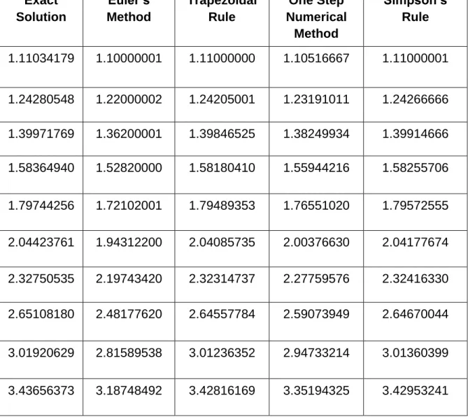
The exact solution is obtained as 𝑦(𝑥) = 2𝑒𝑥− 𝑥 − 1
The results and the errors incurred are shown in Tables 1 and 2 respectively.
Table 1: Results for Problem 1 at 𝒉 = 𝟎. 𝟏
Exact Solution
Euler’s Method
Trapezoidal Rule
One Step Numerical
Method
Simpson’s Rule
1.11034179 1.10000001 1.11000000 1.10516667 1.11000001
1.24280548 1.22000002 1.24205001 1.23191011 1.24266666
1.39971769 1.36200001 1.39846525 1.38249934 1.39914666
1.58364940 1.52820000 1.58180410 1.55944216 1.58255706
1.79744256 1.72102001 1.79489353 1.76551020 1.79572555
2.04423761 1.94312200 2.04085735 2.00376630 2.04177674
2.32750535 2.19743420 2.32314737 2.27759576 2.32416330
2.65108180 2.48177620 2.64557784 2.59073949 2.64670044
3.01920629 2.81589538 3.01236352 2.94733214 3.01360399
http://escipub.com/research-journal-of-mathematics-and-computer-science/ 7 Figure 1: Graphical interpretation of Table 1
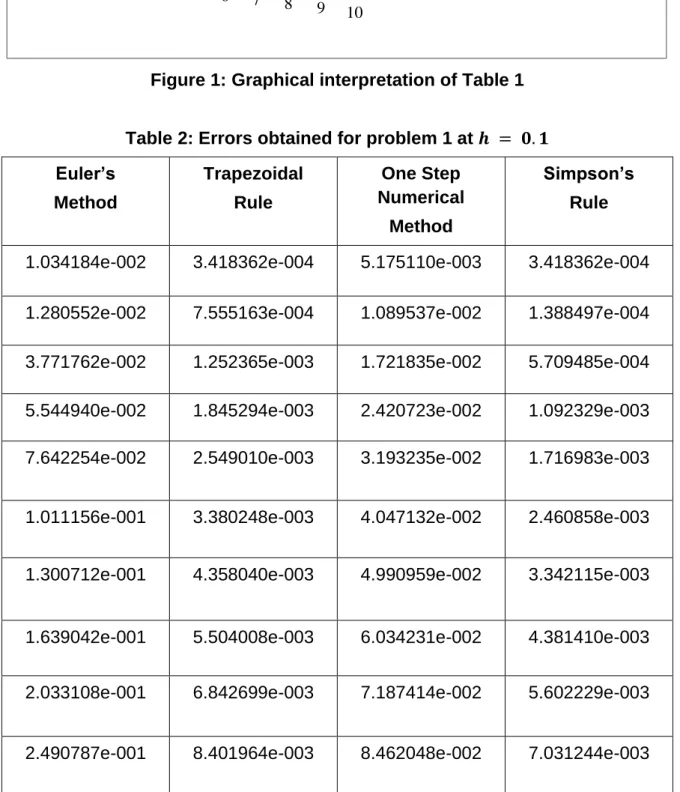
Table 2: Errors obtained for problem 1 at 𝒉 = 𝟎. 𝟏
Euler’s Method
Trapezoidal
Rule
One Step Numerical
Method
Simpson’s Rule
1.034184e-002 3.418362e-004 5.175110e-003 3.418362e-004
1.280552e-002 7.555163e-004 1.089537e-002 1.388497e-004
3.771762e-002 1.252365e-003 1.721835e-002 5.709485e-004
5.544940e-002 1.845294e-003 2.420723e-002 1.092329e-003
7.642254e-002 2.549010e-003 3.193235e-002 1.716983e-003
1.011156e-001 3.380248e-003 4.047132e-002 2.460858e-003
1.300712e-001 4.358040e-003 4.990959e-002 3.342115e-003
1.639042e-001 5.504008e-003 6.034231e-002 4.381410e-003
2.033108e-001 6.842699e-003 7.187414e-002 5.602229e-003
2.490787e-001 8.401964e-003 8.462048e-002 7.031244e-003 0
0.5 1 1.5 2 2.5 3 3.5
1 2 3
4 5 6
7 8 9
10
Exact solution Euler’s method Trapezoidal rule
http://escipub.com/research-journal-of-mathematics-and-computer-science/ 8 Figure 2: Graphical interpretation of Table 2
Example 2
𝑦′= −𝑦 , 𝑦(0) = 1 with ℎ = 0.1
The exact solution is obtained as 𝑦(𝑥) = 𝑒−𝑥
The results and the errors incurred are shown in Tables 3 and 4 respectively.
Table 3: Results for problem 2 at 𝒉 = 𝟎. 𝟏
Exact
Solution
Euler’s Method
Trapezoidal Rule
One Step Numerical
Method
Simpson’s Rule
0.90483743 0.90000000 0.90500000 0.89483333 0.90500000
0.81873077 0.81000001 0.81902500 0.80072665 0.81866666
0.74081820 0.72900001 0.74121762 0.71651691 0.74089333
0.67032003 0.65610000 0.67080195 0.64116323 0.67050846
0.60653067 0.59049000 0.60707576 0.57373422 0.60681016
0.54881161 0.53144100 0.54940356 0.51339650 0.54916319
0.49658531 0.47829690 0.49721022 0.45940429 0.49699269
0.44932896 0.43046721 0.44997525 0.41109028 0.44932896
0.40656966 0.38742048 0.40722760 0.36785728 0.40704944
0.36787945 0.34678440 0.36854098 0.32917094 0.36837974 0.00E+00
5.00E-02 1.00E-01 1.50E-01 2.00E-01 2.50E-01
1 2 3
4 5 6
7 8 9
10
Euler’s method
Trapezoidal rule
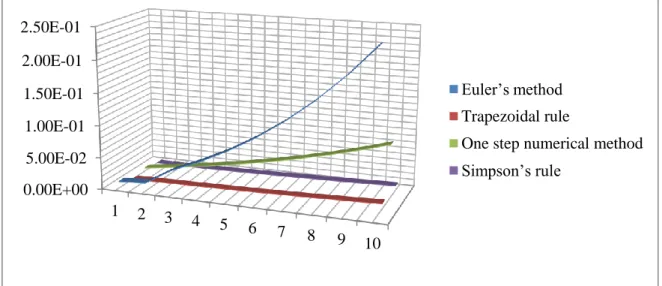
http://escipub.com/research-journal-of-mathematics-and-computer-science/ 9 Figure 3: Graphical interpretation of Table 3
Table 4: Errors obtained for problem 2 at 𝒉 = 𝟎. 𝟏
Euler’s Method
Trapezoidal
Rule
One Step Numerical
Method
Simpson’s Rule
4.837418e-003 1.625820e-004 1.000410e-002 1.625820e-004
8.730753e-003 2.942469e-004 1.800412e-002 6.408641e-005
1.181822e-002 3.994043e-004 2430129e-002 7.511265e-005
1.422005e-002 4.819046e-004 2.915680e-002 1.884206e-004
1.604066e-002 5.451056e-004 3.279644e-002 2.795026e-004
1.737064e-002 5.919315e-004 3.541511e-002 3.515608e-004
1.828840e-004 6.249249e-004 3.718102e-002 4.073894e-004
1.886175e-002 6.462928e-004 3.823867e-002 4.494232e-004
1.914917e-002 6.579478e-004 3871238e-002 4.797808e-004
1.920100e-002 6.615437e-004 3.870851e-002 5.00325e-004 0
0.2 0.4 0.6 0.8 1
1 2 3
4 5
6 7 8
9 10
Exact solution Euler’s method
Trapezoidal rule
http://escipub.com/research-journal-of-mathematics-and-computer-science/ 10 Figure 4: Graphical interpretation of Table 4
4.2 DISCUSSION OF RESULTS AND CONCLUDING REMARKS
In this paper, Euler’s method, Trapezoidal rule, Simpson’s rule and one-step numerical method was used to solve two sampled problems of first order ordinary differential equations in order to compare the results and determine if one-step numerical method is employable to solve such problems. Since the results and errors obtained via the newly developed method shown in Tables 1, 2 and Tables 3, 4 respectively, compared favorably with other existing methods, this shows that the new one step method performs better and is an alternative approach for solving initial value problems in ordinary differential equations. We recommend a further extension to this research in the area of applications. The scheme can still be implemented on other initial and boundary value problems of ordinary differential equations. Moreover, some of the problems arising from biological sciences, engineering and economics can be translated mathematically into an ordinary differential equation and we believe that the scheme could be of help to provide approximate solutions.
Biography
Fadugba Sunday Emmanuel is a Lecturer in the Department of Mathematics, Ekiti State University, Ado Ekiti, Nigeria. He is a registered Member of International Association of Engineers (IAENG). He is also a registered Professional Member of International Technology and Science Publications (ITS). He holds a Ph.D. Degree in Mathematics in the area of Financial Mathematics from the University of Ibadan, Nigeria. His research interests are in Numerical Analysis, Financial Mathematics and Stochastic Analysis with Applications.
Olaosebikan Tayo is a Ph.D. research student in the Department of Mathematics, Ekiti State University, Ado Ekiti, Nigeria. He holds a Master of Science in Mathematics from Ekiti State University, Ado Ekiti, Nigeria. His research interest is in Optimization and Numerical Analysis.
References
1 Aboiyar T., Luga T. and Ivorter B. V. (2015), Derivation of continuous linear multistep methods using Hermite polynomials as basis functions, American Journal of Applied Mathematics and Statistics, 3 (6), 220-225. 2 Butcher, J.C., Numerical Methods for Ordinary
Differential Equation, West Sussex: John Wiley & Sons Ltd, 2003.
0.00E+00 1.00E+04 2.00E+04 3.00E+04 4.00E+04
1 2 3
4 5 6
7 8 9
10
Euler’s method
Trapezoidal rule
http://escipub.com/research-journal-of-mathematics-and-computer-science/ 11 3 Fadugba, S.E. and Falodun, B. O., (2017),
Development of a new one-step scheme for the solution of initial value problem (IVP) in ordinary differential equations, International Journal of Theoretical and Applied Mathematics, 3:58-63. 4 Fatunla, S.O., (1976), A new algorithm for the
numerical solution of ODEs, Computers and Mathematics with Applications, 2: 247-253. 5 Ibijola, E.A. (1997), A new numerical scheme for
the solution of initial value problems (IVPs), Ph.D. Thesis, University of Benin, Nigeria. 6 Ibijola, E.A., (1998), On the convergence,
consistency and stability of a one-step method for Integration of ODEs, International Journal of Computer Mathematics, 73:261-277.
7 Kama, P. and Ibijola, E.A., (2000). On a new one – step Method for numerical integration of ordinary differential equations, International Journal of Computer Mathematics, 78, 21-29. 8 Lambert, J.D., Numerical methods for ordinary
differential systems: the initial value problem. John Wiley & Sons, Inc., New York, 1991. 9 Zarina, B.I., Mohammed, S., Kharil, I. and