Hybrid Feature Selection Approach Based on GRASP for Cancer Microarray Data

Arpita Nagpal and Deepti Gaur

Department of Computer Science and Engineering, School of Engineering and Technology, The NorthCap University, Gurugram, Haryana, India

Hybrid Feature Selection Approach

Based on GRASP for Cancer

Microarray Data

Microarray data usually contain a large number of genes, but a small number of samples. Feature sub-set selection for microarray data aims at reducing the number of genes so that useful information can be ex-tracted from the samples. Reducing the dimension of data sets further helps in improving the computational efficiency of the learning model. In this paper, we pro-pose a modified algorithm based on the tabu search as local search procedures to a Greedy Randomized Adaptive Search Procedure (GRASP) for high dimen-sional microarray data sets. The proposed Tabu based Greedy Randomized Adaptive Search Procedure al-gorithm is named as TGRASP. In TGRASP, a new parameter has been introduced named as Tabu Tenure and the existing parameters, NumIter and size have been modified. We observed that different parameter settings affect the quality of the optimum. The sec-ond proposed algorithm known as FFGRASP (Firefly Greedy Randomized Adaptive Search Procedure) uses a firefly optimization algorithm in the local search op-timization phase of the greedy randomized adaptive search procedure (GRASP). Firefly algorithm is one of the powerful algorithms for optimization of mul-timodal applications. Experimental results show that the proposed TGRASP and FFGRASP algorithms are much better than existing algorithm with respect to three performance parameters viz. accuracy, run time, number of a selected subset of features. We have also compared both the approaches with a unified metric (Extended Adjusted Ratio of Ratios) which has shown that TGRASP approach outperforms existing approach for six out of nine cancer microarray datasets and FF-GRASP performs better on seven out of nine datasets.

ACM CCS (2012) Classification: Theory of computa-tion → Design and analysis of algorithms → Mathe-matical optimization → Discrete optimization → Op-timization with randomized search heuristics

Keywords: feature selection, microarray, classifica-tion, GRASP, hill climbing, firefly algorithm, tabu search

1. Introduction

In recent years, there has been a lot of research in the medical community on microarray data. Many data analysis techniques have been ap-plied to the classification of cancer microar-ray data [1], [2]. The greatest challenge when dealing with microarray data is its very high dimensionality of genes, but small number of samples compared with the large number of genes awakens the curse of dimensionality [3]. When such large number of genes are given as input to machine learning tasks such as clus-tering, or classification, it leads to the problem of overfitting. Also, it increases the classifiers, complexity and the time needed for its training and execution. The presence of irrelevant and redundant genes also affects the performance of the classifier. Hence, the task of feature subset selection becomes important so that the irrele-vant and redundant features are removed. This will further lead to decrease in data acquisition cost and learning time to help in improving can-cer diagnosis.

selec-tion technique, some attributes whose informa-tion overlaps with other attributes called redun-dant attributes are removed from the dataset. It does not transform the features; instead, it helps in improving the accuracy of different classifi-cation tasks. From the dataset of a disease, one is interested in finding the specific features/ genes which are responsible for its occurrence. The high dimensionality of the data makes it difficult to find the specific genes. In case of cancer microarray data, obtaining a transformed set of features using feature extraction does not help and hence dimension reduction is usually carried out using feature/gene selection.

A subset of the features is derived using the val-ues of the features where the value of a feature can be calculated by some mathematical crite-ria. There are different evaluation criteria and according to those criteria, feature selection can be broadly classified into four categories which are filter, wrapper, embedded and hybrid ap-proaches [6], [7], [8].

In filter feature selection, feature subset is se-lected as a preprocessing step before applying any learning and classification process. They become independent of the learning algorithm to be applied. They are usually faster and com-putationally more efficient than wrapper [7]. In the wrapper method [9], like simulated an-nealing or a genetic algorithm, features are selected in accordance with the learning al-gorithm which we are going to apply next. It gives better feature subset than filter approach as it is tuned according to the algorithm, but it is much slower than filter feature selection and has to be rerun when the algorithm changes. When the number of features becomes very large, the filter model is usually chosen due to its computational efficiency and simplicity [8]. In literature, many feature subset selection algo-rithms based on filter and a wrapper approach for different applications have been proposed. All the algorithms aim to remove the irrelevant as well as redundant features from the original set of features and obtain a feature subset. Us-ing the filter feature selection approach, many algorithms were proposed such as Relief [11], Relief-F [12], FOCUS, FOCUS-2 [13], Cor-relation based feature selection (CFS) [14], Fast Correlation based feature selection FCBS [8], FAST [6]. Algorithm by Yang et al. [15]

re-moves irrelevant features based on gene rank-ing methods of GS1 and GS2.

Kohavi and John [9] proposed a wrapper method which removes features from the data-set with the help of the learning algorithm. Its performance is always better than that of fil-ter selection method, but it is computationally more expensive. For solving the gene selection and cancer classification problem, artificial bee colony (ABC) algorithm and minimum redun-dancy maximum relevance (mRMR) algorithm combined together have been proved to be an efficient approach [16]. This is a hybrid ap-proach which offers a balance between filter and wrapper methods. Another hybrid approach which was recently proposed, uses a firefly al-gorithm in its wrapper phase of the alal-gorithm for short term load forecasting application [17]. To take the advantage of the wrapper method, Bermejo, Gamez and Puerta [19] proposed a hybrid algorithm which can speed up the fea-ture selection process. Their method is based on Greedy Randomized Adaptive Search Pro-cedure (GRASP). GRASP is developed in two stages, filter evaluation method is used in the first stage and the solution found here is given as the starting point to a local search method in the next stage. To provide a good quality solu-tion, these two phases are run many times. It tries to move from local optima provided by lo-cal search to a global optimum.

In this paper, we use a multi-start two stage al-gorithm named GRASP (Greedy Randomized Adoptive Search Procedure) [10]. The initial phase of constructing a reduced set of features in TGRASP and FFGRASP algorithms is taken from a fast hybrid algorithm for feature selec-tion in the high dimensional dataset [19]. In the first phase, filter evaluation method of mutual information is used to take out irrelevant fea-tures. Then, a solution to the problem, i.e. a re-duced set of features is constructed using the construction steps used by GRASP algorithm. The solution found is given as input to the local search method for its further improvement. The local search methods used are the tabu search and firefly optimization algorithm. They are computationally less expensive wrapper meth-ods and provide better feature subsets in terms of accuracy as compared to other methods such as hill climbing and simulated annealing. Our aim of this study is to come up with an

opti-approaches. The first phase of this algorithm is taken from a standard hybrid algorithm: In-cremental Wrapper Subset Selection (IWSS) algorithm [25], [26]. The second phase, which is the improvement phase, has been modified so that it takes n wrapper evaluation for each step. In order to have reduced computation time for high dimensional data, it maintains a set of

non-dominated solutions (NDS) in the con -struction phase. Non-dominated set of solution is the set in which every solution in the set is different, in terms of number of features and accuracy. Suppose there are two solutions S1 and S2, S2 is non-dominated by S1 if |S1| ≤ |S2| and accuracy (S1) > accuracy (S2). According to their observations, they have recommended hill climbing as a local search procedure to be used in the improvement phase. We have named their algorithm as FCGRASP that uses a hill climb-ing in its improvement phase.

The FCGRASP algorithm is depicted in Fig-ure 1. The input given to the algorithm is Size: which gives the number of variables to be con-sidered at each iteration and NumIter which gives the number of iterations in both phases. The output of the algorithm is the final selected subset.

In the initialization phase of the algorithm,

NDS is initialized to be empty. The relevance

of each feature with its class label or target fea-ture is calculated and stored in the array named ''relevance''. It is calculated by any filter based approach. Then this relevance value is used to calculate the probability of each feature in the dataset. The probability of occurrence of each feature is stored in the ProbSel array.

Now the construction and improvement phases are performed till the number of iterations spec-ified by the user is over. The construction phase is depicted in lines 7 to 16. In each iteration, construction phase adds a new solution to the

NDS. Line 7 selects the subset of features from

X determined by the parameter Size and stores it in subset variable. A feature is selected based on its value in ''ProbSel'' array. The features in subset variable are sorted and stored in array R. The function evaluate (C,S,D) calculates the classification accuracy of the dataset D over classifier C with S variables using 5-cross val-idation. Then, using the loop from second fea-ture to last, it is checked whether a feafea-ture im-mization technique for microarray dataset that

decreases the number of wrapper evaluations without affecting the accuracy. Tabu search and firefly algorithms have proved to have bet-ter accuracy than hill climbing as local search methods.

The rest of the paper is organized as follows: Section 2 gives a detailed description of the GRASP algorithm along with an existing fast hybrid algorithm. Section 3 discusses the pro-posed algorithms TGRASP and FFGRASP. Section 4 gives the description of the cancer microarray datasets along with the experimen-tal results and comparisons found with the ex-isting algorithm. Finally, in Section 5 we draw conclusions based on the experimental results.

2. GRASP Algorithm for Feature

Selection

GRASP is a meta heuristic algorithm devel-oped in two stages. It was develdevel-oped by Feo and Resende [10], [20]. Further, GRASP has been used to develop many applications [21], [22]. The two stages of the GRASP algo-rithm are the construction phase and the improvement phase.

1. Construction phase: In this stage, a solu-tion with reduced features is constructed using some heuristic approaches. It starts from an empty set and keeps on adding el-ements till a solution is obtained.

2. Improvement Phase: The result obtained in the construction phase is modified using some local search algorithm.

Esseghir and Casado-Yusta have proposed a feature subset selection (FSS) algorithm based on the technique of GRASP [23], [24]. In their algorithm, for the construction phase, they have used filter algorithm such as Relief [11] and FCBF [8]. For the improvement phase, some wrapper techniques were applied. The draw-back of these two proposed algorithms is that they do not work well if the data is high dimen-sional.

tion technique, some attributes whose informa-tion overlaps with other attributes called redun-dant attributes are removed from the dataset. It does not transform the features; instead, it helps in improving the accuracy of different classifi-cation tasks. From the dataset of a disease, one is interested in finding the specific features/ genes which are responsible for its occurrence. The high dimensionality of the data makes it difficult to find the specific genes. In case of cancer microarray data, obtaining a transformed set of features using feature extraction does not help and hence dimension reduction is usually carried out using feature/gene selection.

A subset of the features is derived using the val-ues of the features where the value of a feature can be calculated by some mathematical crite-ria. There are different evaluation criteria and according to those criteria, feature selection can be broadly classified into four categories which are filter, wrapper, embedded and hybrid ap-proaches [6], [7], [8].

In filter feature selection, feature subset is se-lected as a preprocessing step before applying any learning and classification process. They become independent of the learning algorithm to be applied. They are usually faster and com-putationally more efficient than wrapper [7]. In the wrapper method [9], like simulated an-nealing or a genetic algorithm, features are selected in accordance with the learning al-gorithm which we are going to apply next. It gives better feature subset than filter approach as it is tuned according to the algorithm, but it is much slower than filter feature selection and has to be rerun when the algorithm changes. When the number of features becomes very large, the filter model is usually chosen due to its computational efficiency and simplicity [8]. In literature, many feature subset selection algo-rithms based on filter and a wrapper approach for different applications have been proposed. All the algorithms aim to remove the irrelevant as well as redundant features from the original set of features and obtain a feature subset. Us-ing the filter feature selection approach, many algorithms were proposed such as Relief [11], Relief-F [12], FOCUS, FOCUS-2 [13], Cor-relation based feature selection (CFS) [14], Fast Correlation based feature selection FCBS [8], FAST [6]. Algorithm by Yang et al. [15]

re-moves irrelevant features based on gene rank-ing methods of GS1 and GS2.

Kohavi and John [9] proposed a wrapper method which removes features from the data-set with the help of the learning algorithm. Its performance is always better than that of fil-ter selection method, but it is computationally more expensive. For solving the gene selection and cancer classification problem, artificial bee colony (ABC) algorithm and minimum redun-dancy maximum relevance (mRMR) algorithm combined together have been proved to be an efficient approach [16]. This is a hybrid ap-proach which offers a balance between filter and wrapper methods. Another hybrid approach which was recently proposed, uses a firefly al-gorithm in its wrapper phase of the alal-gorithm for short term load forecasting application [17]. To take the advantage of the wrapper method, Bermejo, Gamez and Puerta [19] proposed a hybrid algorithm which can speed up the fea-ture selection process. Their method is based on Greedy Randomized Adaptive Search Pro-cedure (GRASP). GRASP is developed in two stages, filter evaluation method is used in the first stage and the solution found here is given as the starting point to a local search method in the next stage. To provide a good quality solu-tion, these two phases are run many times. It tries to move from local optima provided by lo-cal search to a global optimum.

In this paper, we use a multi-start two stage al-gorithm named GRASP (Greedy Randomized Adoptive Search Procedure) [10]. The initial phase of constructing a reduced set of features in TGRASP and FFGRASP algorithms is taken from a fast hybrid algorithm for feature selec-tion in the high dimensional dataset [19]. In the first phase, filter evaluation method of mutual information is used to take out irrelevant fea-tures. Then, a solution to the problem, i.e. a re-duced set of features is constructed using the construction steps used by GRASP algorithm. The solution found is given as input to the local search method for its further improvement. The local search methods used are the tabu search and firefly optimization algorithm. They are computationally less expensive wrapper meth-ods and provide better feature subsets in terms of accuracy as compared to other methods such as hill climbing and simulated annealing. Our aim of this study is to come up with an

opti-approaches. The first phase of this algorithm is taken from a standard hybrid algorithm: In-cremental Wrapper Subset Selection (IWSS) algorithm [25], [26]. The second phase, which is the improvement phase, has been modified so that it takes n wrapper evaluation for each step. In order to have reduced computation time for high dimensional data, it maintains a set of

non-dominated solutions (NDS) in the con -struction phase. Non-dominated set of solution is the set in which every solution in the set is different, in terms of number of features and accuracy. Suppose there are two solutions S1 and S2, S2 is non-dominated by S1 if |S1| ≤ |S2| and accuracy (S1) > accuracy (S2). According to their observations, they have recommended hill climbing as a local search procedure to be used in the improvement phase. We have named their algorithm as FCGRASP that uses a hill climb-ing in its improvement phase.

The FCGRASP algorithm is depicted in Fig-ure 1. The input given to the algorithm is Size: which gives the number of variables to be con-sidered at each iteration and NumIter which gives the number of iterations in both phases. The output of the algorithm is the final selected subset.

In the initialization phase of the algorithm,

NDS is initialized to be empty. The relevance

of each feature with its class label or target fea-ture is calculated and stored in the array named ''relevance''. It is calculated by any filter based approach. Then this relevance value is used to calculate the probability of each feature in the dataset. The probability of occurrence of each feature is stored in the ProbSel array.

Now the construction and improvement phases are performed till the number of iterations spec-ified by the user is over. The construction phase is depicted in lines 7 to 16. In each iteration, construction phase adds a new solution to the

NDS. Line 7 selects the subset of features from

X determined by the parameter Size and stores it in subset variable. A feature is selected based on its value in ''ProbSel'' array. The features in subset variable are sorted and stored in array R. The function evaluate (C,S,D) calculates the classification accuracy of the dataset D over classifier C with S variables using 5-cross val-idation. Then, using the loop from second fea-ture to last, it is checked whether a feafea-ture im-mization technique for microarray dataset that

decreases the number of wrapper evaluations without affecting the accuracy. Tabu search and firefly algorithms have proved to have bet-ter accuracy than hill climbing as local search methods.

The rest of the paper is organized as follows: Section 2 gives a detailed description of the GRASP algorithm along with an existing fast hybrid algorithm. Section 3 discusses the pro-posed algorithms TGRASP and FFGRASP. Section 4 gives the description of the cancer microarray datasets along with the experimen-tal results and comparisons found with the ex-isting algorithm. Finally, in Section 5 we draw conclusions based on the experimental results.

2. GRASP Algorithm for Feature

Selection

GRASP is a meta heuristic algorithm devel-oped in two stages. It was develdevel-oped by Feo and Resende [10], [20]. Further, GRASP has been used to develop many applications [21], [22]. The two stages of the GRASP algo-rithm are the construction phase and the improvement phase.

1. Construction phase: In this stage, a solu-tion with reduced features is constructed using some heuristic approaches. It starts from an empty set and keeps on adding el-ements till a solution is obtained.

2. Improvement Phase: The result obtained in the construction phase is modified using some local search algorithm.

Esseghir and Casado-Yusta have proposed a feature subset selection (FSS) algorithm based on the technique of GRASP [23], [24]. In their algorithm, for the construction phase, they have used filter algorithm such as Relief [11] and FCBF [8]. For the improvement phase, some wrapper techniques were applied. The draw-back of these two proposed algorithms is that they do not work well if the data is high dimen-sional.

proves the classification accuracy or not. If it improves the accuracy, it is added to S.

Lines 17 to 20 perform the improving step.

Here the value of solution S returned by

con-struction step is added to NDS if and only if the

solution is not present in the non-dominated set.

Update function modifies NDS and improving

method is executed with S as starting point in line 19. This improving method is one of the lo-cal-search based FSS algorithm. There are dif-ferent choices for local-search based algorithms such as hill climbing [19], genetic algorithms and simulated annealing. We have found that hill climbing has some drawbacks.

● Possibility of being trapped at a local opti-mum as it performs only a single run of the iterative improvement.

● There is no chance of an escape from local minima.

● It may cycle over the same solutions again and again and thus become redundant The drawbacks found in case of using simu-lated annealing as a local search algorithm are:

● The result found using simulated anneal-ing can vary on each run of the algorithm, in other words, every run of simulated an-nealing gives a different solution.

● Only under certain circumstances, the op-timum solution is found. So, you may have to run the algorithm many times to obtain the optimum solution.

3. The Proposed Method

To overcome the drawbacks of hill climbing and simu-lated annealing used in the improve-ment phase of GRASP, we have adopted tabu search optimization and firefly optimization approaches in the improvement phase of the GRASP algorithm.

3.1. Tabu Search Based GRASP Approach (TGRASP)

The tabu search uses neighborhood search like simulated annealing and hill climbing, but also uses memory to record the history. So, the ma-jor advantage of using this technique is that the number of solutions to be tested keeps re-ducing. This is because it uses memory called tabu list, that records the recent history of the search and cycling back to previously visited solutions is avoided. In many practical prob-lems, it is seen that a reasonable size tabu list improves the performance of hill climbing. For high dimensional datasets like microarray data, the solution obtained by tabu search rivals and often surpasses the best solutions previously found by simulated annealing and hill climbing. Using tabu search we can avoid repeating the search. By using tabu list as used in tabu search approach, the problem of redundancy can be re-moved from the hill climbing approach. In gen-eral, tabu list has a fixed size to memorize, and it follows FIFO in maintaining the list.

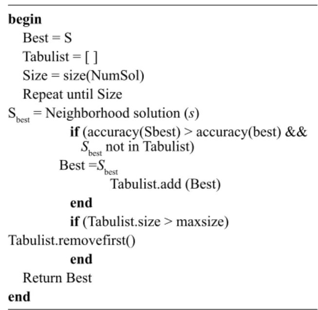
The pseudo code of the algorithm is demon-strated in Figure 2. Initially the first solution

found in the list of all possible solutions is taken as the best solution. Tabu list is initialized to be empty.

Tabu search stops when all the solutions found

in non-dominated set (NDS) have been evalu -ated. If the accuracy of the new solution Sbest, is better than the accuracy of the best solution last found, then the best solution is replaced with the new solution (Sbest). We also check that the new solution (Sbest) is not presented in the existing tabu list before making it a best solu-tion. This new solution is then added in the tabu list.

Here, we have used short term tabu list, which keeps record of last 20 solutions. The advan-tage of using tabu list is that the repeated solu-tions are not checked again. When the solution reaches the maximum size of the list, then the first added solution from the tabu list is de-leted. The algorithm returns the best solution out of the solutions found in the construction of GRASP.

3.2. Novel Firefly Algorithm

In this section, we present a discrete firefly algorithm (FFGRASP) for the improvement phase of the GRASP algorithm. Yang and He

[27] have surveyed and shown that firefly algo-rithm has been used in many applications and produces better performance in terms of time and optimality than other algorithms.

It obtains better global results than simulated annealing, PSO and artificial bee colony (ABC) algorithm. Firefly algorithm is a bio-inspired optimization algorithm proposed by Xin-She Yang at Cambridge University [28], [29]. It is based on the pattern of flashing light of fire-flies. This algorithm focuses on two important issues obtained from the behaviour of fireflies: the variation of light intensity and formulation of the attractiveness. The attractiveness of two fireflies is proportional to the brightness of the fireflies. The lesser bright fireflies move to-wards the brighter ones. If there is no brighter one than a particular firefly, it will move ran-domly. Further, brightness is determined by the light intensity of the fireflies which affects the objective function f. Brightness, li of a firefly i at location y is given by l(y) ∝ f(y). Attractive-ness β, is determined by the adjacent fireflies and it varies with distance rij between firefly i and firefly j.

Exploration is the acquisition of new informa-tion through searching. Explorainforma-tion is a main concern for all optimizers because it might lead to new search regions that might contain better solutions. Exploitation is defined as the applica-tion of known informaapplica-tion. The good sites are exploited via the application of a local search [30]. Variation in the light intensity controls the tradeoff between exploration and exploitation in the firefly algorithm. The firefly i is attracted to another brighter firefly j, its position at itera-tion t + 1 is determined by:

2

( )

( 1)t t rij ₍ t t₎ t

i i o j i t i

x + ₌x ₊β e−γ x ₋x _{+ ∈}α

(1) The second component of the equation 1 is the exploration and it is used for attraction between the two fireflies. The parameters used in this part are β and γ. β is the attractiveness which is proportional to the light intensity seen by other fireflies. βo is the attractiveness at r = 0. γ controls the average distance of a group of fire-flies that can be seen by adjacent groups. The distance between two fireflies is the Cartesian distance which is given as:

In D: Data set; F: filter measure; C:class label /target feature;

Size: number of variables to consider at each iteration;

numIt: number of iterations in algorithm Out S : The selected subset

// initialization

1. NDS = NULL 2. for each Xi∈X

3. Relevance [i] = F(Xi, C) + Ɛ

4. for each Xi∈X

5. ProbSel [i] = Relevance [i] / ∑n_j =1 Relevance [j]

// GRASP

6. for i = 1 to numIt

// constructive step

7. subset = some Size features selected using ProbSel [ ] from X without replacement 8. R [ ] = rank the features based on scores value 9. S = R [1]

10. BestValue = evaluate(C, S, D) 11. for i_r = 2 to R.size ()

12. Saux = S∪R_ir

13. NewValue = evaluate (C, Saux, D) 14. if (NewValue > BestValue) then

15. S = Saux

16. BestValue = NewValue

// improving step

17. if (update (NDS, S)) then

18. Xnds = ∪_si∈ NDS S_ir

19. S' = ExecuteImprovingMethod (Xnds, S, C, D) 20. update (NDS, S')

21. return all or best solution(s) in NDS

Figure 1. FCGRASP algorithm for FSS.

Input: S: Start State

NumSol: List of all possible solutions Output: Best: an improved solution

begin

Best = S Tabulist = [ ] Size = size(NumSol) Repeat until Size

S_best = Neighborhood solution (s)

if (accuracy(Sbest) > accuracy(best) && S_best not in Tabulist)

Best =Sbest

Tabulist.add (Best) end

if (Tabulist.size > maxsize) Tabulist.removefirst()

end

Return Best

end

proves the classification accuracy or not. If it improves the accuracy, it is added to S.

Lines 17 to 20 perform the improving step.

Here the value of solution S returned by

con-struction step is added to NDS if and only if the

solution is not present in the non-dominated set.

Update function modifies NDS and improving

method is executed with S as starting point in line 19. This improving method is one of the lo-cal-search based FSS algorithm. There are dif-ferent choices for local-search based algorithms such as hill climbing [19], genetic algorithms and simulated annealing. We have found that hill climbing has some drawbacks.

● Possibility of being trapped at a local opti-mum as it performs only a single run of the iterative improvement.

● There is no chance of an escape from local minima.

● It may cycle over the same solutions again and again and thus become redundant The drawbacks found in case of using simu-lated annealing as a local search algorithm are:

● The result found using simulated anneal-ing can vary on each run of the algorithm, in other words, every run of simulated an-nealing gives a different solution.

● Only under certain circumstances, the op-timum solution is found. So, you may have to run the algorithm many times to obtain the optimum solution.

3. The Proposed Method

To overcome the drawbacks of hill climbing and simu-lated annealing used in the improve-ment phase of GRASP, we have adopted tabu search optimization and firefly optimization approaches in the improvement phase of the GRASP algorithm.

3.1. Tabu Search Based GRASP Approach (TGRASP)

The tabu search uses neighborhood search like simulated annealing and hill climbing, but also uses memory to record the history. So, the ma-jor advantage of using this technique is that the number of solutions to be tested keeps re-ducing. This is because it uses memory called tabu list, that records the recent history of the search and cycling back to previously visited solutions is avoided. In many practical prob-lems, it is seen that a reasonable size tabu list improves the performance of hill climbing. For high dimensional datasets like microarray data, the solution obtained by tabu search rivals and often surpasses the best solutions previously found by simulated annealing and hill climbing. Using tabu search we can avoid repeating the search. By using tabu list as used in tabu search approach, the problem of redundancy can be re-moved from the hill climbing approach. In gen-eral, tabu list has a fixed size to memorize, and it follows FIFO in maintaining the list.

The pseudo code of the algorithm is demon-strated in Figure 2. Initially the first solution

found in the list of all possible solutions is taken as the best solution. Tabu list is initialized to be empty.

Tabu search stops when all the solutions found

in non-dominated set (NDS) have been evalu -ated. If the accuracy of the new solution Sbest, is better than the accuracy of the best solution last found, then the best solution is replaced with the new solution (Sbest). We also check that the new solution (Sbest) is not presented in the existing tabu list before making it a best solu-tion. This new solution is then added in the tabu list.

Here, we have used short term tabu list, which keeps record of last 20 solutions. The advan-tage of using tabu list is that the repeated solu-tions are not checked again. When the solution reaches the maximum size of the list, then the first added solution from the tabu list is de-leted. The algorithm returns the best solution out of the solutions found in the construction of GRASP.

3.2. Novel Firefly Algorithm

In this section, we present a discrete firefly algorithm (FFGRASP) for the improvement phase of the GRASP algorithm. Yang and He

[27] have surveyed and shown that firefly algo-rithm has been used in many applications and produces better performance in terms of time and optimality than other algorithms.

It obtains better global results than simulated annealing, PSO and artificial bee colony (ABC) algorithm. Firefly algorithm is a bio-inspired optimization algorithm proposed by Xin-She Yang at Cambridge University [28], [29]. It is based on the pattern of flashing light of fire-flies. This algorithm focuses on two important issues obtained from the behaviour of fireflies: the variation of light intensity and formulation of the attractiveness. The attractiveness of two fireflies is proportional to the brightness of the fireflies. The lesser bright fireflies move to-wards the brighter ones. If there is no brighter one than a particular firefly, it will move ran-domly. Further, brightness is determined by the light intensity of the fireflies which affects the objective function f. Brightness, li of a firefly i at location y is given by l(y) ∝ f(y). Attractive-ness β, is determined by the adjacent fireflies and it varies with distance rij between firefly i and firefly j.

Exploration is the acquisition of new informa-tion through searching. Explorainforma-tion is a main concern for all optimizers because it might lead to new search regions that might contain better solutions. Exploitation is defined as the applica-tion of known informaapplica-tion. The good sites are exploited via the application of a local search [30]. Variation in the light intensity controls the tradeoff between exploration and exploitation in the firefly algorithm. The firefly i is attracted to another brighter firefly j, its position at itera-tion t + 1 is determined by:

2

( )

( 1)t t rij ₍ t t₎ t

i i o j i t i

x + ₌x ₊β e−γ x ₋x _{+ ∈}α

(1) The second component of the equation 1 is the exploration and it is used for attraction between the two fireflies. The parameters used in this part are β and γ. β is the attractiveness which is proportional to the light intensity seen by other fireflies. βo is the attractiveness at r = 0. γ controls the average distance of a group of fire-flies that can be seen by adjacent groups. The distance between two fireflies is the Cartesian distance which is given as:

In D: Data set; F: filter measure; C:class label /target feature;

Size: number of variables to consider at each iteration;

numIt: number of iterations in algorithm Out S : The selected subset

// initialization

1. NDS = NULL 2. for each Xi∈X

3. Relevance [i] = F(Xi, C) + Ɛ

4. for each Xi∈X

5. ProbSel [i] = Relevance [i] / ∑n_j =1 Relevance [j]

// GRASP

6. for i = 1 to numIt

// constructive step

7. subset = some Size features selected using ProbSel [ ] from X without replacement 8. R [ ] = rank the features based on scores value 9. S = R [1]

10. BestValue = evaluate(C, S, D) 11. for i_r = 2 to R.size ()

12. Saux = S∪R_ir

13. NewValue = evaluate (C, Saux, D) 14. if (NewValue > BestValue) then

15. S = Saux

16. BestValue = NewValue

// improving step

17. if (update (NDS, S)) then

18. Xnds = ∪_si∈ NDS S_ir

19. S' = ExecuteImprovingMethod (Xnds, S, C, D) 20. update (NDS, S')

21. return all or best solution(s) in NDS

Figure 1. FCGRASP algorithm for FSS.

Input: S: Start State

NumSol: List of all possible solutions Output: Best: an improved solution

begin

Best = S Tabulist = [ ] Size = size(NumSol) Repeat until Size

S_best = Neighborhood solution (s)

if (accuracy(Sbest) > accuracy(best) && S_best not in Tabulist)

Best =Sbest

Tabulist.add (Best) end

if (Tabulist.size > maxsize) Tabulist.removefirst()

end

Return Best

end

2

, ,

1( )

d

i k j k

k

∑

= x −x (2) The third component of the equation 1 is the ex-ploitation. Exploitation is controlled by the ran-domization parameter αt, which is tuned during each iteration so that it can vary with iteration counter t.

In our implementation, the objective function is the average accuracy obtained through the clas-sifier, naïve Bayes and SVM. We have taken

βo = 1 as used by most of the applications. The parameters γ and α have been used in the algo-rithm such that they are dependent on the num-ber of features selected at each iteration.

Parameters γ and α are updated at each iteration as follows:

1. Gamma parameter (γ) is given by, 1/ z

γ = where Z = (|D| – |di|)/|D| where |D| is the total number of features. |di| is the number of features selected at each itera-tion. Iteration (i) varies from 1 to Numiter, Numiter is the number of iterations.

2. Alpha parameter (∝) is given by, ∝ =

(1 – ∆)Z, ∆ is the cooling factor for ran

-domness. We have used ∆ = 0.98 in the ex -periments performed here.

Formally, the modified discrete firefly algo-rithm as used in the improvement phase of the GRASP is given in Figure 3.

4. Empirical Study

An existing hybrid algorithm, which uses hill climbing as a local search procedure in the im-provement phase of GRASP named FCGRASP has been used to com-pare the proposed algo-rithms. In this section, we have compared our proposed algorithms named TGRASP and FF-GRASP with FCFF-GRASP on different publically available cancer datasets.

4.1. Experimental Setup and Dataset

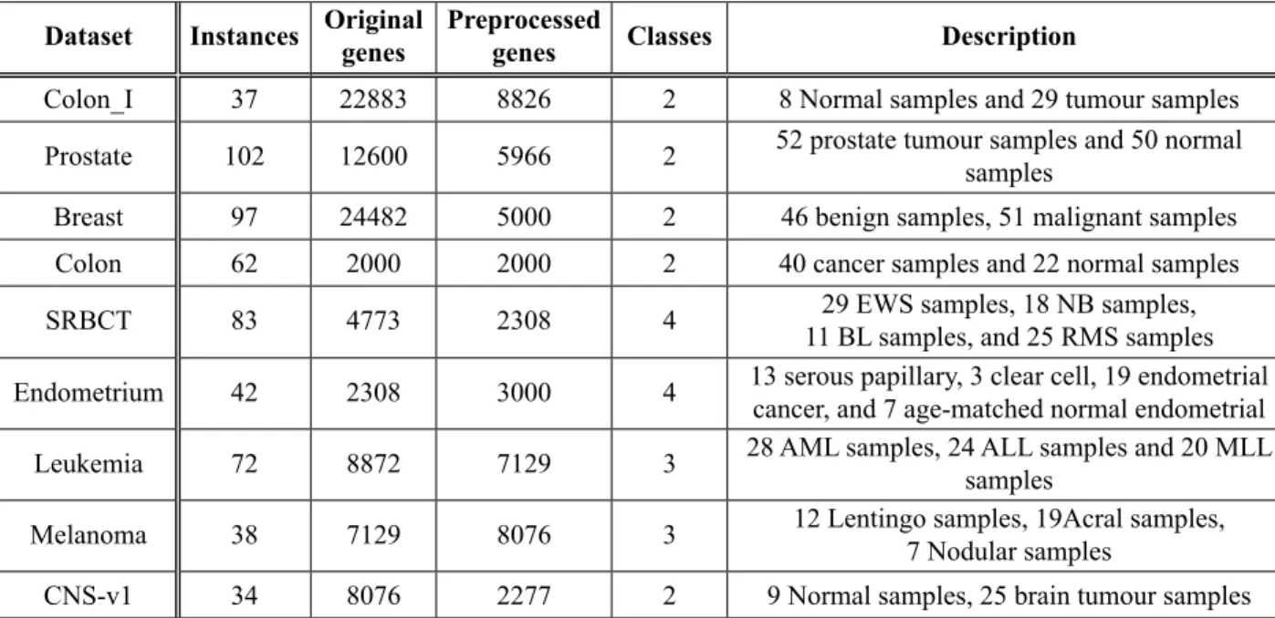
The experiments have been performed on nine cancer microarray datasets of high dimensions. The data set is described in Table 1. Some

datasets have two classes, while some have

more than two classes. Datasets are obtained

from different sources. Breast, colon, leukemia and prostate datasets were obtained from Kent

Ridge Biomedical Dataset data repository [31].

For SRBCT, Khan dataset has been used [2]. Table 1 gives the further details about these datasets.

Before actually using the data in the exper-iments, a preprocessing procedure has been

applied to them. Datasets of breast and en -dometrium contained null values. The attributes containing more than 30% missing values have been left out. Other null values were replaced with the class wise mean of their respective attributes. Thus, 3000 attributes were left for endometrium and 5000 for breast cancer data

[32]. Data for colon, SRBCT, leukemia and

melanoma were used as they were. For other datasets, we adopted the technique suggested by Yang et al. [15] and Ramaswamy et al. [33].

For prostate dataset, floor value of 100 and a ceiling value of 16000 with a variation of the Max /Min ratio as 5 and Max-Min difference of 50 were used to filter the values. CNS-v1, Colon-I used the intensity threshold value as floor and ceiling between 20 – 16000 with Max/Min ratio as 5, 3 and Max-Min difference of 500, 100 respectively. All datasets were nor-malized using z-score normalization before us-ing them in ex-periments.

The algorithms FCGRASP and TGRASP are implemented in matlab on the same PC. Classi-fication algorithms embedded in wrapper eval-uation are created as functions in matlab and are called wherever needed.

The parameters used to compare both algo-rithms are the number of features, runtime and classification accuracy. Runtime is machine dependent, so we have implemented and com-pared both algorithms on the same machine. The classification accuracy is calculated using 10 fold cross validation strategy for the train-ing and testtrain-ing sets. The traintrain-ing set consists of 90% of the values and the test set consist of 10% of values. For each classification al-gorithm, we obtain the average classification accuracy, number of selected features, runtime found under each algorithm and each dataset. One parameter named EARR (Extended Ad-justed Ratio of Ratios) proposed by Wang [34] has also been used to compare both algorithms.

It is a multicriteria metric, where the classifica-tion accuracy, runtime and number of features selected are integrated. EARR evaluates the performance by taking the ratio of the metric

values. Let D = {D1,D2,….,Dn} be a set of n datasets, and A ={A1, A2, …., An) be a set of M FSS algorithms. Then, the EARR of Ai to Aj over Dk can be defined as:

,

/

, 1 .log( / ) .log( / )

(1 , 1 )

Dk

i j

k k i j

A A k k k k i j i j

acc acc EARR

t t n n

i j M k N

β =

+ ∝ +

≤ ≠ ≤ ≤ <

(3)

∝ and β are user defined parameters which tell us how much the runtime and number of fea-tures selected should respectively dominate ac-curacy. accik is the accuracy of ith _{algorithm of} kth _{dataset. t}

ik and nik are the runtime and number of selected features of dataset k on ith _algorithm respectively. The greater the value of EARR, the better the corresponding algorithm on a given dataset D [34].

As discussed in the algorithm, we have used Symmetric Uncertainty (SU) for the filter eval-uation [6], [8]. For the wrapper phase, Naïve Bayes and Support Vector Machine (SVM) classifiers are used. Support vector machine performs very well on most of the problems in high dimensional space. It is difficult to find a linear classifier to separate different classes

Input:

• Initial Values to parameters: α the randomness parameter, β the attraction coefficient, γ the parameter to control randomness, ∆ = 0.98 • Objective function f (y), y_i= (y₁, y₂, ..., y_d)T

• All solutions in NDS, S_i = (S₁, S₂, ..., S_n) Output: Best solution set S_best

begin

Calculate light intensityli at y_i by f(y_i) S_best = NULL

While (t < numiter)

for i = 1:n // all n solutions at this step for j = 1:i

Determine the position of i using equation

if ( l_i > I_j)

Move firefly i towards j in all d dimensions Sbest = Si

Else

Change position of i randomly

endif

Determine new solutions from NDS and revise light intensity

endj

endi

Return Sbest

Calculate new α and γ values

end while

Figure 3. Discrete firefly algorithm in the improvement phase.

Table 1. Dataset description.

Dataset Instances Original _genes Preprocessed _genes Classes Description

Colon_I 37 22883 8826 2 8 Normal samples and 29 tumour samples

Prostate 102 12600 5966 2 52 prostate tumour samples and 50 normal _samples

Breast 97 24482 5000 2 46 benign samples, 51 malignant samples

Colon 62 2000 2000 2 40 cancer samples and 22 normal samples

SRBCT 83 4773 2308 4 _{11 BL samples, and 25 RMS samples}29 EWS samples, 18 NB samples,

Endometrium 42 2308 3000 4 13 serous papillary, 3 clear cell, 19 endometrial _{cancer, and 7 age-matched normal endometrial}

Leukemia 72 8872 7129 3 28 AML samples, 24 ALL samples and 20 MLL _samples

Melanoma 38 7129 8076 3 12 Lentingo samples, 19Acral samples,_{7 Nodular samples}

2

, ,

1( )

d

i k j k

k

∑

= x −x (2) The third component of the equation 1 is the ex-ploitation. Exploitation is controlled by the ran-domization parameter αt, which is tuned during each iteration so that it can vary with iteration counter t.

In our implementation, the objective function is the average accuracy obtained through the clas-sifier, naïve Bayes and SVM. We have taken

βo = 1 as used by most of the applications. The parameters γ and α have been used in the algo-rithm such that they are dependent on the num-ber of features selected at each iteration.

Parameters γ and α are updated at each iteration as follows:

1. Gamma parameter (γ) is given by, 1/ z

γ = where Z = (|D| – |di|)/|D| where |D| is the total number of features. |di| is the number of features selected at each itera-tion. Iteration (i) varies from 1 to Numiter, Numiter is the number of iterations.

2. Alpha parameter (∝) is given by, ∝ =

(1 – ∆)Z, ∆ is the cooling factor for ran

-domness. We have used ∆ = 0.98 in the ex -periments performed here.

Formally, the modified discrete firefly algo-rithm as used in the improvement phase of the GRASP is given in Figure 3.

4. Empirical Study

An existing hybrid algorithm, which uses hill climbing as a local search procedure in the im-provement phase of GRASP named FCGRASP has been used to com-pare the proposed algo-rithms. In this section, we have compared our proposed algorithms named TGRASP and FF-GRASP with FCFF-GRASP on different publically available cancer datasets.

4.1. Experimental Setup and Dataset

The experiments have been performed on nine cancer microarray datasets of high dimensions. The data set is described in Table 1. Some

datasets have two classes, while some have

more than two classes. Datasets are obtained

from different sources. Breast, colon, leukemia and prostate datasets were obtained from Kent

Ridge Biomedical Dataset data repository [31].

For SRBCT, Khan dataset has been used [2]. Table 1 gives the further details about these datasets.

Before actually using the data in the exper-iments, a preprocessing procedure has been

applied to them. Datasets of breast and en -dometrium contained null values. The attributes containing more than 30% missing values have been left out. Other null values were replaced with the class wise mean of their respective attributes. Thus, 3000 attributes were left for endometrium and 5000 for breast cancer data

[32]. Data for colon, SRBCT, leukemia and

melanoma were used as they were. For other datasets, we adopted the technique suggested by Yang et al. [15] and Ramaswamy et al. [33].

For prostate dataset, floor value of 100 and a ceiling value of 16000 with a variation of the Max /Min ratio as 5 and Max-Min difference of 50 were used to filter the values. CNS-v1, Colon-I used the intensity threshold value as floor and ceiling between 20 – 16000 with Max/Min ratio as 5, 3 and Max-Min difference of 500, 100 respectively. All datasets were nor-malized using z-score normalization before us-ing them in ex-periments.

The algorithms FCGRASP and TGRASP are implemented in matlab on the same PC. Classi-fication algorithms embedded in wrapper eval-uation are created as functions in matlab and are called wherever needed.

The parameters used to compare both algo-rithms are the number of features, runtime and classification accuracy. Runtime is machine dependent, so we have implemented and com-pared both algorithms on the same machine. The classification accuracy is calculated using 10 fold cross validation strategy for the train-ing and testtrain-ing sets. The traintrain-ing set consists of 90% of the values and the test set consist of 10% of values. For each classification al-gorithm, we obtain the average classification accuracy, number of selected features, runtime found under each algorithm and each dataset. One parameter named EARR (Extended Ad-justed Ratio of Ratios) proposed by Wang [34] has also been used to compare both algorithms.

It is a multicriteria metric, where the classifica-tion accuracy, runtime and number of features selected are integrated. EARR evaluates the performance by taking the ratio of the metric

values. Let D = {D1,D2,….,Dn} be a set of n datasets, and A ={A1, A2, …., An) be a set of M FSS algorithms. Then, the EARR of Ai to Aj over Dk can be defined as:

,

/

, 1 .log( / ) .log( / )

(1 , 1 )

Dk

i j

k k i j

A A k k k k i j i j

acc acc EARR

t t n n

i j M k N

β =

+ ∝ +

≤ ≠ ≤ ≤ <

(3)

∝ and β are user defined parameters which tell us how much the runtime and number of fea-tures selected should respectively dominate ac-curacy. accik is the accuracy of ith _{algorithm of} kth _{dataset. t}

ik and nik are the runtime and number of selected features of dataset k on ith _algorithm respectively. The greater the value of EARR, the better the corresponding algorithm on a given dataset D [34].

As discussed in the algorithm, we have used Symmetric Uncertainty (SU) for the filter eval-uation [6], [8]. For the wrapper phase, Naïve Bayes and Support Vector Machine (SVM) classifiers are used. Support vector machine performs very well on most of the problems in high dimensional space. It is difficult to find a linear classifier to separate different classes

Input:

• Initial Values to parameters: α the randomness parameter, β the attraction coefficient, γ the parameter to control randomness, ∆ = 0.98 • Objective function f (y), y_i= (y₁, y₂, ..., y_d)T

• All solutions in NDS, S_i = (S₁, S₂, ..., S_n) Output: Best solution set S_best

begin

Calculate light intensityli at y_i by f(y_i) S_best = NULL

While (t < numiter)

for i = 1:n // all n solutions at this step for j = 1:i

Determine the position of i using equation

if ( l_i > I_j)

Move firefly i towards j in all d dimensions Sbest = Si

Else

Change position of i randomly

endif

Determine new solutions from NDS and revise light intensity

endj

endi

Return Sbest

Calculate new α and γ values

end while

Figure 3. Discrete firefly algorithm in the improvement phase.

Table 1. Dataset description.

Dataset Instances Original _genes Preprocessed _genes Classes Description

Colon_I 37 22883 8826 2 8 Normal samples and 29 tumour samples

Prostate 102 12600 5966 2 52 prostate tumour samples and 50 normal _samples

Breast 97 24482 5000 2 46 benign samples, 51 malignant samples

Colon 62 2000 2000 2 40 cancer samples and 22 normal samples

SRBCT 83 4773 2308 4 _{11 BL samples, and 25 RMS samples}29 EWS samples, 18 NB samples,

Endometrium 42 2308 3000 4 13 serous papillary, 3 clear cell, 19 endometrial _{cancer, and 7 age-matched normal endometrial}

Leukemia 72 8872 7129 3 28 AML samples, 24 ALL samples and 20 MLL _samples

Melanoma 38 7129 8076 3 12 Lentingo samples, 19Acral samples,_{7 Nodular samples}

in the dataset. This problem can be solved us-ing SVM. It is proved to be relatively new and promising classifier over other classifiers [18]. Naïve Bayes is quite sensitive to the presence of redundant and irrelevant predicted attributes [19].

4.2. Experimental Results

The proposed algorithms TGRASP and FF-GRASP have been compared with an existing algorithm FCGRASP. They have been com-pared in terms of three performance measures, i.e., classification accuracy, runtime and num-ber of features. The classifiers used are Naïve Bayes classifier and SVM.

In all of the three algorithms, Size and NumIter are the parameters used to carry out multiple wrapper evaluations. Tabu tenure is a param-eter that is used only for TGRASP algorithm. Tabu tenure is the length of the tabu list kept at the time of performing the experiments. This parameter is a static tabu list with short term memory for storing a maximum of 20 values. In our experiments, we have varied the size of the tabu tenure from 5 to 15. For most of the datasets, we observed that after the size of Tabu tenure reaches 10, the solutions repeat them-selves. So, to compare all datasets on a com-mon value of Tabu tenure, we have shown the results when its value was 8.

Table 2 and Table 3 give the comparison of TGRASP, FFGRASP and FCGRASP by keep-ing the value of tabu tenure as 8. NumIter parameter is fixed to 50 and then 100 for all datasets and for both classifiers. The value of parameter ''Size'' varies based on the total num-ber of features in each dataset.

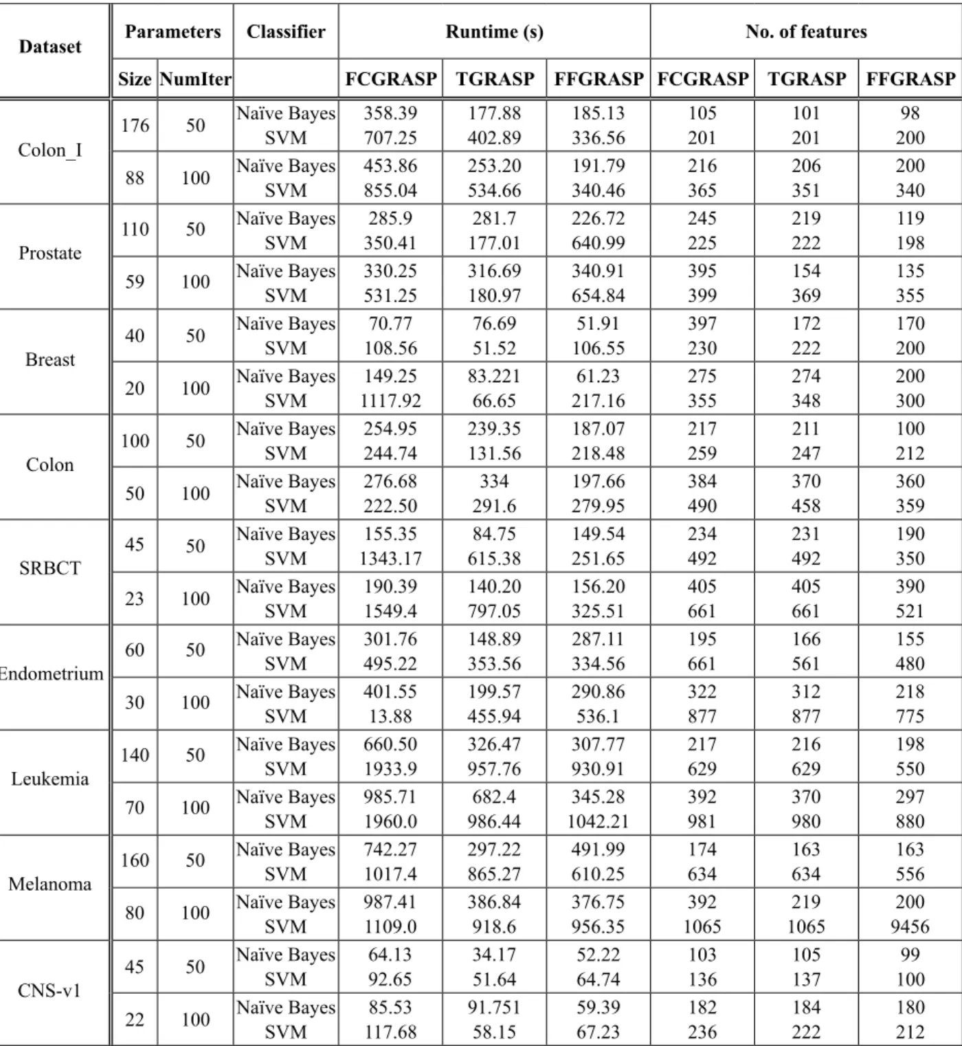
Table 2 gives the average number of features and average runtime in seconds obtained using 10 fold cross validation. From the results we observe that

● As the number of iterations (NumIter) in-creased from 50 to 100, it showed a sig-nificant change in the number of wrapper evaluation and hence we could observe that there was approximately 25 – 30% in-crease in runtime in most of the datasets.

● In case of two class dataset, when Nu-mIter = 50, and Naïve classifier was con-sidered, the average runtime of FFGRASP

decreased by 13.2, 27.7 percent over TGRASP and FCGRASP respectively. The runtime of TGRASP in case of SVM Clas-sifier has been decreased by 84.5, 67.8 per-cent of that of FCGRASP and FFGRASP respectively.

● For four class dataset, when Naïve Bayes classifier was used, TGRASP ranks 1. Its average runtime over both the datasets decreased by 95.6, 86.9 percent of that of FCGRASP and FFGRASP respectively. When SVM classifier was considered, FF-GRASP has a decreased average runtime by 65.2, 21.38 percent by TGRASP and FCGRASP respectively.

● In all the datasets, FFGRASP algorithm selects less number of features in the range of 2 to 227 numbers of features, as com-pared to FCGRASP.

● In the majority of the datasets, on average, approximately 80 percent of the features selected by FFGRASP and TGRASP are common with the features selected by FC-GRASP.

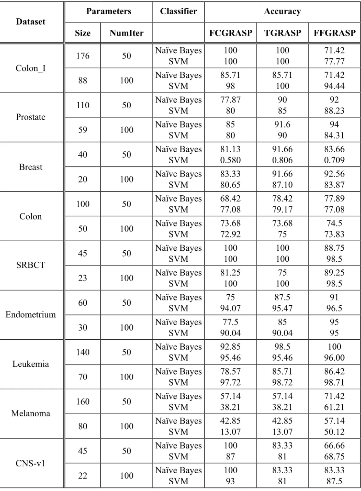
Table 3 shows the average accuracy of the three algorithms found using 10 fold cross validation of two classifiers on nine cancer datasets. The results observed using Naïve Bayes classifier are as follows:

● For two class datasets, when NumIter = 50, as compared to FCGRASP, the classi-fication accuracy of Naïve Bayes has been improved by TGRASP algorithm by 12, 15, 14 percent in case of colon, prostate and breast datasets respectively. TGRASP shows an improvement over FFGRASP in classification accuracy by 40, 9.4 and 1 percent for colon_I, colon and breast datasets respectively. FFGRASP has in-creased the classification accuracy in case of prostate dataset by 18 and 2 percent from FCGRASP and TGRASP respectively. However, CNS-v1 is the only two class dataset which has decreased the classifica-tion accuracy of TGRASP and FFGRASP by 20 and 50.01 percent respectively from FCGRASP.

● For two class datasets, when NumIter = 100, the classification accuracy of Naïve Bayes has been improved by TGRASP algorithm by 7 and 9 percent in case of

prostate and colon datasets respectively. FFGRASP shows an improvement over FCGRASP in the range of 1 to 11 percent. Unfortunately, in case of dataset CNS-v1 the accuracy of TGRASP and FFGRASP has been decreased by 20 percent from FC-GRASP.

● In case of endometrium dataset, FFGRASP classification accuracy has been improved

by 21.3 and 4 percent from FCGRASP and TGRASP respectively when NumIter = 50. The accuracy was improved by 22.5 and 5.5 percent from FCGRASP and TGRASP respectively when NumIter = 100.

● For SRBCT dataset, when NumIter = 50, maximum classification accuracy of 100% was achieved by FCGRASP and TGRASP algo-rithms, and the accuracy Table 2. Comparison of FCGRASP, TGRASP and FFGRASP in terms of runtime and number of features

selected when NumIter = 50 and 100.

Dataset Parameters Classifier Runtime (s) No. of features

Size NumIter FCGRASP TGRASP FFGRASP FCGRASP TGRASP FFGRASP

Colon_I 176 50

Naïve Bayes

SVM 358.39 707.25 177.88 402.89 185.13 336.56 105 201 101 201 20098 88 100 Naïve Bayes _SVM 453.86 _855.04 253.20 _534.66 191.79 _340.46 216 ₃₆₅ 206 ₃₅₁ 200 ₃₄₀

Prostate 110 50

Naïve Bayes

SVM 350.41285.9 177.01281.7 226.72 640.99 245 225 219 222 119 198 59 100 Naïve Bayes _SVM 330.25 _531.25 316.69 _180.97 340.91 _654.84 395 ₃₉₉ 154 ₃₆₉ 135 ₃₅₅

Breast 40 50

Naïve Bayes

SVM 108.5670.77 76.69 51.52 106.5551.91 397 230 172 222 170 200 20 100 Naïve Bayes _{SVM 1117.92}149.25 83.221 _{66.65 217.16}61.23 275 ₃₅₅ 274 ₃₄₈ 200 ₃₀₀

Colon 100 50

Naïve Bayes

SVM 254.95 244.74 239.35 131.56 187.07 218.48 217 259 211 247 100 212 50 100 Naïve Bayes _SVM 276.68 _{222.50 291.6}334 197.66 _279.95 384 ₄₉₀ 370 ₄₅₈ 360 ₃₅₉

SRBCT 45 50

Naïve Bayes

SVM 1343.17155.35 615.3884.75 149.54 251.65 234 492 231 492 190 350 23 100 Naïve Bayes _SVM 190.39 _1549.4 140.20 _797.05 156.20 _325.51 405 ₆₆₁ 405 ₆₆₁ 390 ₅₂₁

Endometrium 60 50

Naïve Bayes

SVM 301.76 495.22 148.89 353.56 287.11 334.56 195 661 166 561 155 480 30 100 Naïve Bayes _SVM 401.55 _13.88 199.57 _455.94 290.86 _536.1 322 ₈₇₇ 312 ₈₇₇ 218 ₇₇₅

Leukemia 140 50

Naïve Bayes

SVM 660.50 1933.9 326.47 957.76 307.77 930.91 217 629 216 629 198 550 70 100 Naïve Bayes _SVM 985.71 _{1960.0 986.44}682.4 _1042.21345.28 392 ₉₈₁ 370 ₉₈₀ 297 ₈₈₀

Melanoma 160 50

Naïve Bayes

SVM 742.27 1017.4 297.22 865.27 491.99 610.25 174 634 163 634 163 556 80 100 Naïve Bayes

SVM 987.41 1109.0 386.84 918.6 376.75 956.35 1065392 1065219 9456200

CNS-v1 45 50

Naïve Bayes

in the dataset. This problem can be solved us-ing SVM. It is proved to be relatively new and promising classifier over other classifiers [18]. Naïve Bayes is quite sensitive to the presence of redundant and irrelevant predicted attributes [19].

4.2. Experimental Results

The proposed algorithms TGRASP and FF-GRASP have been compared with an existing algorithm FCGRASP. They have been com-pared in terms of three performance measures, i.e., classification accuracy, runtime and num-ber of features. The classifiers used are Naïve Bayes classifier and SVM.

In all of the three algorithms, Size and NumIter are the parameters used to carry out multiple wrapper evaluations. Tabu tenure is a param-eter that is used only for TGRASP algorithm. Tabu tenure is the length of the tabu list kept at the time of performing the experiments. This parameter is a static tabu list with short term memory for storing a maximum of 20 values. In our experiments, we have varied the size of the tabu tenure from 5 to 15. For most of the datasets, we observed that after the size of Tabu tenure reaches 10, the solutions repeat them-selves. So, to compare all datasets on a com-mon value of Tabu tenure, we have shown the results when its value was 8.

Table 2 and Table 3 give the comparison of TGRASP, FFGRASP and FCGRASP by keep-ing the value of tabu tenure as 8. NumIter parameter is fixed to 50 and then 100 for all datasets and for both classifiers. The value of parameter ''Size'' varies based on the total num-ber of features in each dataset.

Table 2 gives the average number of features and average runtime in seconds obtained using 10 fold cross validation. From the results we observe that

● As the number of iterations (NumIter) in-creased from 50 to 100, it showed a sig-nificant change in the number of wrapper evaluation and hence we could observe that there was approximately 25 – 30% in-crease in runtime in most of the datasets.

● In case of two class dataset, when Nu-mIter = 50, and Naïve classifier was con-sidered, the average runtime of FFGRASP

decreased by 13.2, 27.7 percent over TGRASP and FCGRASP respectively. The runtime of TGRASP in case of SVM Clas-sifier has been decreased by 84.5, 67.8 per-cent of that of FCGRASP and FFGRASP respectively.

● For four class dataset, when Naïve Bayes classifier was used, TGRASP ranks 1. Its average runtime over both the datasets decreased by 95.6, 86.9 percent of that of FCGRASP and FFGRASP respectively. When SVM classifier was considered, FF-GRASP has a decreased average runtime by 65.2, 21.38 percent by TGRASP and FCGRASP respectively.

● In all the datasets, FFGRASP algorithm selects less number of features in the range of 2 to 227 numbers of features, as com-pared to FCGRASP.

● In the majority of the datasets, on average, approximately 80 percent of the features selected by FFGRASP and TGRASP are common with the features selected by FC-GRASP.

Table 3 shows the average accuracy of the three algorithms found using 10 fold cross validation of two classifiers on nine cancer datasets. The results observed using Naïve Bayes classifier are as follows:

● For two class datasets, when NumIter = 50, as compared to FCGRASP, the classi-fication accuracy of Naïve Bayes has been improved by TGRASP algorithm by 12, 15, 14 percent in case of colon, prostate and breast datasets respectively. TGRASP shows an improvement over FFGRASP in classification accuracy by 40, 9.4 and 1 percent for colon_I, colon and breast datasets respectively. FFGRASP has in-creased the classification accuracy in case of prostate dataset by 18 and 2 percent from FCGRASP and TGRASP respectively. However, CNS-v1 is the only two class dataset which has decreased the classifica-tion accuracy of TGRASP and FFGRASP by 20 and 50.01 percent respectively from FCGRASP.

● For two class datasets, when NumIter = 100, the classification accuracy of Naïve Bayes has been improved by TGRASP algorithm by 7 and 9 percent in case of

prostate and colon datasets respectively. FFGRASP shows an improvement over FCGRASP in the range of 1 to 11 percent. Unfortunately, in case of dataset CNS-v1 the accuracy of TGRASP and FFGRASP has been decreased by 20 percent from FC-GRASP.

● In case of endometrium dataset, FFGRASP classification accuracy has been improved

by 21.3 and 4 percent from FCGRASP and TGRASP respectively when NumIter = 50. The accuracy was improved by 22.5 and 5.5 percent from FCGRASP and TGRASP respectively when NumIter = 100.

● For SRBCT dataset, when NumIter = 50, maximum classification accuracy of 100% was achieved by FCGRASP and TGRASP algo-rithms, and the accuracy Table 2. Comparison of FCGRASP, TGRASP and FFGRASP in terms of runtime and number of features

selected when NumIter = 50 and 100.

Dataset Parameters Classifier Runtime (s) No. of features

Size NumIter FCGRASP TGRASP FFGRASP FCGRASP TGRASP FFGRASP

Colon_I 176 50

Naïve Bayes

SVM 358.39 707.25 177.88 402.89 185.13 336.56 105 201 101 201 20098 88 100 Naïve Bayes _SVM 453.86 _855.04 253.20 _534.66 191.79 _340.46 216 ₃₆₅ 206 ₃₅₁ 200 ₃₄₀

Prostate 110 50

Naïve Bayes

SVM 350.41285.9 177.01281.7 226.72 640.99 245 225 219 222 119 198 59 100 Naïve Bayes _SVM 330.25 _531.25 316.69 _180.97 340.91 _654.84 395 ₃₉₉ 154 ₃₆₉ 135 ₃₅₅

Breast 40 50

Naïve Bayes

SVM 108.5670.77 76.69 51.52 106.5551.91 397 230 172 222 170 200 20 100 Naïve Bayes _{SVM 1117.92}149.25 83.221 _{66.65 217.16}61.23 275 ₃₅₅ 274 ₃₄₈ 200 ₃₀₀

Colon 100 50

Naïve Bayes

SVM 254.95 244.74 239.35 131.56 187.07 218.48 217 259 211 247 100 212 50 100 Naïve Bayes _SVM 276.68 _{222.50 291.6}334 197.66 _279.95 384 ₄₉₀ 370 ₄₅₈ 360 ₃₅₉

SRBCT 45 50

Naïve Bayes

SVM 1343.17155.35 615.3884.75 149.54 251.65 234 492 231 492 190 350 23 100 Naïve Bayes _SVM 190.39 _1549.4 140.20 _797.05 156.20 _325.51 405 ₆₆₁ 405 ₆₆₁ 390 ₅₂₁

Endometrium 60 50

Naïve Bayes

SVM 301.76 495.22 148.89 353.56 287.11 334.56 195 661 166 561 155 480 30 100 Naïve Bayes _SVM 401.55 _13.88 199.57 _455.94 290.86 _536.1 322 ₈₇₇ 312 ₈₇₇ 218 ₇₇₅

Leukemia 140 50

Naïve Bayes

SVM 660.50 1933.9 326.47 957.76 307.77 930.91 217 629 216 629 198 550 70 100 Naïve Bayes _SVM 985.71 _{1960.0 986.44}682.4 _1042.21345.28 392 ₉₈₁ 370 ₉₈₀ 297 ₈₈₀

Melanoma 160 50

Naïve Bayes

SVM 742.27 1017.4 297.22 865.27 491.99 610.25 174 634 163 634 163 556 80 100 Naïve Bayes

SVM 987.41 1109.0 386.84 918.6 376.75 956.35 1065392 1065219 9456200

CNS-v1 45 50

Naïve Bayes

of FFGRASP has been decreased by 12.67 percent. When NumIter = 100, the classi-fication accuracy of FFGRASP has been increased by 9.84 and 19 percent from FC-GRASP and TFC-GRASP respectively.

● In case of three class dataset, when Nu-mIter = 50, the classification accuracy of FFGRASP has shown an improvement

over FCGRASP and TGRASP by 7.7 and 1.5 percent respectively in leukemia data-set and by 24.9 percent over both the algo-rithms in melanoma dataset.

● For three class dataset, when NumIter = 100, FFGRASP takes over by 9.9 and 0.8 percent over FCGRAS and TGRASP respectively for leukemia dataset and by

33.3 percent over FCGRAS and TGRASP for melanoma dataset.

When we consider SVM Classifier in Table 3, we observe that:

● For two class datasets, when NumIter = 50, TGRASP algorithm classification ac-curacy is better than FCGRASP and FF-GRASP in the range of 2 to 29 percent in case of prostate, colon and breast datasets. For colon_I dataset, TGRASP and

FC-GRASP have maximum accuracy of 100%, which has been increased from FFGRASP by 28.58 percent. For dataset, CNS-v1 the classification accuracy of TGRASP and FFGRASP has been decreased by 7.4 and 26.5 percent respectively from FCGRASP.

● For two class datasets, when NumIter=100, Classification accuracy has been improved by TGRASP as compared to FCGRASP by 2, 12, 8, 4 percent for colon_I, prostate, Table 3. Comparison of FCGRASP, TGRASP and FFGRASP in terms of accuracy when numIter = 50 and 100.

Dataset Parameters Classifier Accuracy

Size NumIter FCGRASP TGRASP FFGRASP

Colon_I 176 50

Naïve Bayes

SVM 100 100 100 100 71.42 77.77 88 100 Naïve Bayes _SVM 85.71 ₉₈ 85.71 ₁₀₀ 71.42 _94.44

Prostate 110 50

Naïve Bayes

SVM 77.87 80 90 85 88.2392 59 100 Naïve Bayes _SVM 85 ₈₀ 91.6 _{90 84.31}94

Breast 40 50

Naïve Bayes

SVM 81.13 0.580 91.66 0.806 83.66 0.709 20 100 Naïve Bayes _SVM 83.33 _80.65 91.66 _87.10 92.56 _83.87

Colon

100 50 Naïve Bayes _SVM 68.42 _77.08 78.42 _79.17 77.89 _77.08

50 100 Naïve Bayes _SVM 73.68 _72.92 73.68 _{75 73.83}74.5

SRBCT 45 50

Naïve Bayes

SVM 100 100 100 100 88.75 98.5 23 100 Naïve Bayes _SVM 81.25 _{100 100}75 89.25 _98.5

Endometrium 60 50

Naïve Bayes

SVM 94.0775 95.4787.5 96.591 30 100 Naïve Bayes _{SVM 90.04}77.5 _90.0485 95 ₉₅

Leukemia 140 50

Naïve Bayes

SVM 92.85 95.46 95.4698.5 96.00100 70 100 Naïve Bayes _SVM 78.57 _97.72 85.71 _98.72 86.42 _98.71

Melanoma 160 50

Naïve Bayes

SVM 57.14 38.21 57.14 38.21 71.42 61.21 80 100 Naïve Bayes _SVM 42.85 _13.07 42.85 _13.07 57.14 _50.12

CNS-v1

45 50 Naïve Bayes _SVM 100 ₈₇ 83.33 ₈₁ 66.66 _68.75

22 100 Naïve Bayes _SVM 100 ₉₃ 83.33 ₈₁ 83.33 _87.5

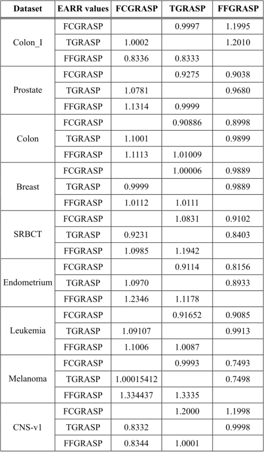
Table 4. EARR Values calculated to compare both the algorithms on all datasets.

Dataset EARR values FCGRASP TGRASP FFGRASP

Colon_I

FCGRASP 0.9997 1.1995

TGRASP 1.0002 1.2010

FFGRASP 0.8336 0.8333

Prostate

FCGRASP 0.9275 0.9038

TGRASP 1.0781 0.9680

FFGRASP 1.1314 0.9999

Colon

FCGRASP 0.90886 0.8998

TGRASP 1.1001 0.9899

FFGRASP 1.1113 1.01009

Breast

FCGRASP 1.00006 0.9889

TGRASP 0.9999 0.9889

FFGRASP 1.0112 1.0111

SRBCT

FCGRASP 1.0831 0.9102

TGRASP 0.9231 0.8403

FFGRASP 1.0985 1.1942

Endometrium

FCGRASP 0.9114 0.8156

TGRASP 1.0970 0.8933

FFGRASP 1.2346 1.1178

Leukemia

FCGRASP 0.91652 0.9085

TGRASP 1.09107 0.9913

FFGRASP 1.1006 1.0087

Melanoma

FCGRASP 0.9993 0.7493

TGRASP 1.00015412 0.7498

FFGRASP 1.334437 1.3335

CNS-v1

FCGRASP 1.2000 1.1998

TGRASP 0.8332 0.9998