RISK SHARING AND EFFICIENCY IMPLICATIONS

R

ISK SHARING AND EFFICIENCY IMPLICATIONS

OF PROGRESSIVE PENSION ARRANGEMENTS

H

F

C

H

CONTENTS 1 / 18

C

1. MOTIVATION

2. THE NUMERICAL GENERAL EQUILIBRIUM MODEL

3. SIMULATION RESULTS

MOTIVATION 2 / 18

M

Fenge (1995): Intragenerational fair paygo system is Pareto-efficient!

Question: Why do we observe progressive pension systems in many

countries?

First answer: Progressivity is determined by the voting outcome

(Casamatta et al., 2000 or Conde-Ruiz and Galasso, 2005).

Here: Pension progressivity is efficient due to it’s insurance

MOTIVATION 3 / 18

Net replacement rates by Basic

individual earnings level allowance

Multiple of average in % of 0.5 1.0 2.0 average wage Germany 61.7 71.8 67.0 10.0a Italy 89.3 88.8 89.1 – Netherlands 82.5 84.1 83.8 – Poland 69.6 69.7 70.5 – Spain 88.7 88.3 83.4 – Australia 77.0 52.4 36.5 – France 98.0 68.8 59.2 – Ireland 63.0 36.6 21.9 55.4 Japan 80.1 59.1 44.3 – UK 78.4 47.6 29.8 22.8 USA 61.4 51.0 39.0 – a_{currently proposed}

MOTIVATION 4 / 18

R

L

• Pension reforms:

Huggett/Ventura (1999), Støresletten et al. (1999), De Nardi et al. (1999), Conesa/Krueger (1999).

• Income tax reforms:

THE NUMERICAL GENERAL EQUILIBRIUM MODEL 5 / 18

T

• Households work for 8 periods (i.e. 40 years) and can live up to 16

periods (i.e. up to age 100),

• Liquidity constraints, unintended bequest;

• Closed economy without population ageing;

• Cobb-Douglas production function with capital and labor,

• Government issues debt and levies progressive income taxes, corporate

THE NUMERICAL GENERAL EQUILIBRIUM MODEL 6 / 18

I

State variables: z = (ep_j, a_j, e_j) earning points, assets, and productivity

Budget constraint:

aj+1 = aj(1 + r) + (1 −j)wej wj

THE NUMERICAL GENERAL EQUILIBRIUM MODEL 7 / 18

M

• Computation of earning points at age j:

epj = epj−1 + min[wj/w¯; 2.0] (1 − λ) + λ

• Computation of individual pension at age j ≥ j_R:

pj = epj_R × AP A

• Computation of individual contribution rate τ_j:

τj = ⎧ ⎨ ⎩ 0 if w_j < βw,¯ τ[wj − βw¯]/wj if βw¯ ≤ wj ≤ 2.0 ¯w, τ[2.0 − β] ¯w/wj if wj > 2.0 ¯w.

THE NUMERICAL GENERAL EQUILIBRIUM MODEL 8 / 18

C

: T

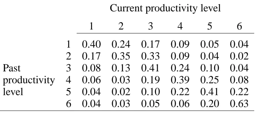
Table 1: Markov transition matrix

Current productivity level

1 2 3 4 5 6 1 0.40 0.24 0.17 0.09 0.05 0.04 2 0.17 0.35 0.33 0.09 0.04 0.02 Past 3 0.08 0.13 0.41 0.24 0.10 0.04 productivity 4 0.06 0.03 0.19 0.39 0.25 0.08 level 5 0.04 0.02 0.10 0.22 0.41 0.22 6 0.04 0.03 0.05 0.06 0.20 0.63

Source: Authors’ own calculations from 1998/2003 SOEP data

SIMULATION RESULTS 9 / 18

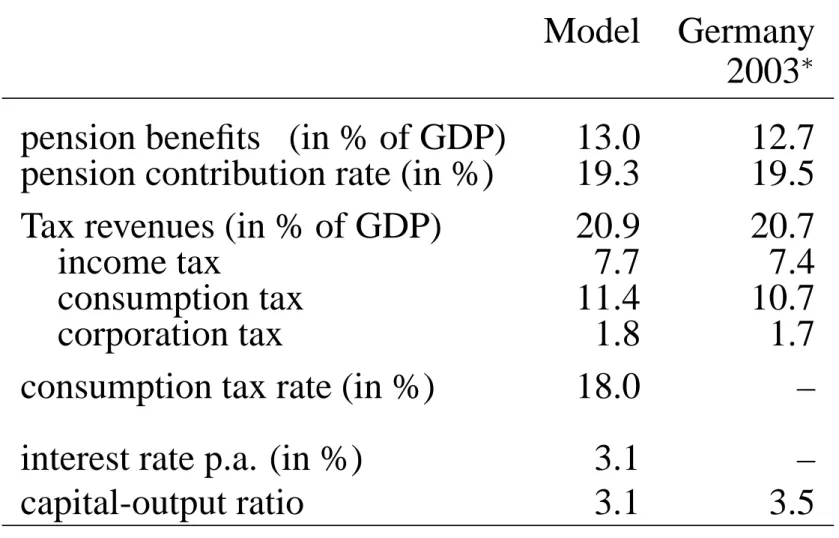
Table 2: The initial equilibrium

Model Germany

2003∗

pension benefits (in % of GDP) 13.0 12.7

pension contribution rate (in %) 19.3 19.5

Tax revenues (in % of GDP) 20.9 20.7

income tax 7.7 7.4

consumption tax 11.4 10.7

corporation tax 1.8 1.7

consumption tax rate (in %) 18.0 –

interest rate p.a. (in %) 3.1 –

capital-output ratio 3.1 3.5

SIMULATION RESULTS 10 / 18

Table 3: Income and Wealth Distribution

Percentage shares Gini

Lowest 10% Highest 10% index

Net income 3.4 22.2 0.287 Model Assets 0.0 30.4 0.518 Net income 3.1 23.9 0.299 Germany∗ Assets 0.2 44.2 0.613 * Source: DIW (2005, 202)

SIMULATION RESULTS 11 / 18

Table 4: Macroeconomic effects of progressive pensions

(β = 0.3, λ = 0.5) Period 2005-09 2025-29 2045-49 ∞ Employment -5.2 -4.1 -4.1 -4.1 Capital stock 0.0 -5.5 -6.6 -7.4 Wagea 1.6 -0.4 -0.8 -1.1 Contribution rate 9.6 9.3 9.3 9.8 Consumption tax 2.0 2.0 2.2 2.3

SIMULATION RESULTS 12 / 18

Figure 1: Welfare effects of progressive pensions

- 3 - 2 - 1 0 1 2 3 1 9 1 0 1 9 3 5 1 9 6 0 1 9 8 5 2 0 1 0 2 0 3 5 Y e a r o f B i r t h A ve ra ge W el fa re C ha ng es in %

SIMULATION RESULTS 13 / 18

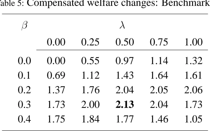
Table 5: Compensated welfare changes: Benchmark∗

β λ 0.00 0.25 0.50 0.75 1.00 0.0 0.00 0.55 0.97 1.14 1.32 0.1 0.69 1.12 1.43 1.64 1.61 0.2 1.37 1.76 2.04 2.05 2.06 0.3 1.73 2.00 2.13 2.04 1.73 0.4 1.75 1.84 1.77 1.46 1.05

SIMULATION RESULTS 14 / 18

D

E

Insurance + liquidity + labor supply effect

−1.49 −1.00 2.13 Sensitivity Analysis: γ : 0.5 → 0.25 ⇒ 2.87 (Liquidity effect ↑)

ρ : 0.6 → 0.7 ⇒ 1.41 (Labor supply effect ↑)

SIMULATION RESULTS 15 / 18

Figure 2: Voting without increasing debt

0 . 0 0 . 2 0 . 4 0 . 6 0 . 8 1 . 0 1 9 1 0 1 9 2 0 1 9 3 0 1 9 4 0 1 9 5 0 1 9 6 0 1 9 7 0 1 9 8 0 Y e a r o f B i r t h Pr o-Fr ac tio n of C oh or ts /V ot er s P r o - F r a c t i o n o f C o h o r t s P r o - F r a c t i o n o f V o t e r s

SIMULATION RESULTS 16 / 18

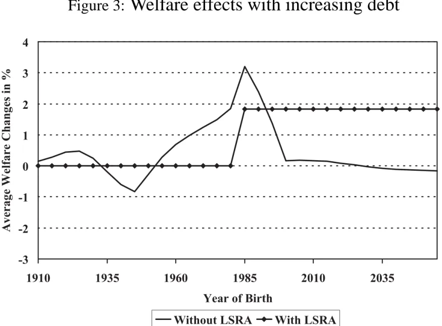
Figure 3: Welfare effects with increasing debt

- 3 - 2 - 1 0 1 2 3 4 1 9 1 0 1 9 3 5 1 9 6 0 1 9 8 5 2 0 1 0 2 0 3 5 Y e a r o f B i r t h A ve ra ge W el fa re C ha ng es in %

SIMULATION RESULTS 17 / 18

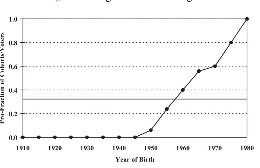
Figure 4: Voting with increasing debt

0 . 0 0 . 2 0 . 4 0 . 6 0 . 8 1 . 0 1 9 1 0 1 9 2 0 1 9 3 0 1 9 4 0 1 9 5 0 1 9 6 0 1 9 7 0 1 9 8 0 Y e a r o f B i r t h Pr o-Fr ac tio n of C oh or ts /V ot er s P r o - F r a c t i o n o f C o h o r t s P r o - F r a c t i o n o f V o t e r s

CONCLUSIONS 18 / 18

C

• Tax-benefit linkage of the German pension system should be reduced!

• Result is robust and reinforced by sensitivity analysis!

• However, such a reform will not find political support!

• Future work:

pension privatization;

optimal progressivity of tax and pension system; mandatory vs. voluntary retirement accounts;