digital project V1,R4 Quick Start

(1)

Q u i c k S t a r t

digital

(2)

Quick Starting Your Knowledge in

Digital Project™ V1,R4

(3)

ii iii

Model Building Steps

1

13 4

10 13

15 16

17 12

11

7 2

5 10

16

6 3

9

9 8 3

(5)

vi vii

Introduction

Digital Project™ is a multi-faceted modeling environment with many paths to achieve the same goal. With that said, the steps in this tutorial are carefully chosen to give the

user rapid results. Please pay close attention to the order in which the instructions are presented.

Installation from Download

Follow these steps for installing Digital Project™ V1,R4

from the website:

• Confirm you have at least 8 GB of free space to down -load, decompress and install the application.

• Go to “Downloads” location under “Support”on Gehry Technologies website (www.gehrytechnologies.com). • Choose 32 or 64 bit depending on the type of operating

system you are running.

• Click and save to your local drive.

• Double click downloaded self-extracting “.exe” file for installer to be extracted onto your local drive.

• The installation program will automatically start up. • For a local project standards install continue with instal

-lation and choose “Install Project Standards” locally when

prompted.

• For shared project standards cancel install program and double click “Readme.bat” in the “DPV1R4_32bit_in

-staller” folder. Select “Install Project Standard” to install project standards first in non-default location (e.g. net

-work drive). Then run “Install Digital Project™ V1,R4”. Choose “Existing Project Standards” and navigate to the

shared directory.

• Contact Gehry Technologies for the purchase of a license if you do not already have one.

(6)

viii ix

Installation from CD

Follow these steps for installing Digital Project™ V1,R4

from a CD:

• Confirm you have at least 4 GB of free space. • Insert the CD.

• An HTML page will pop up with two options: “Install Digital Project™ V1,R4” and “Install Project Standard”. (If HTML page does not open go to the “DPV1R4_32bit_in

-staller” folder and double click “Readme.bat”.)

• Choose “Install Digital Project™ V1,R4” for a stand alone standard install. When prompted in the installation pro

-cess, choose “Install Project Standards” locally. (“Install Digital Project™ V1,R4” is set to launch “SetupApp32. exe” for 32-bit and “SetupApp64.exe” for 64-bit.) • Choose “Install Project Standard” to install project stan

-dards first in non-default location (e.g. network drive). Then run “Install Digital Project™ V1,R4”. Choose “Existing Project Standards” and navigate to the shared directory. (“Install Project Standard” is set to launch “setupStdsEx.exe”.)

• Contact Gehry Technologies for the purchase of a license if you do not already have one.

License Request

To request the purchase of a license for Digital Project™ V1,R4 fill out the license request form on the Gehry Tech

-nologies website (www.gehrytech-nologies.com) under the “Support” tab. Choose the user category (i.e. Commercial or Academic) that applies to you.

License Setup Issues

If you receive this error: “You have not requested a configu -ration or product license. Click OK and select at least one

configuration license using the License Manager dialog box.” Click OK. A “License Manager” will pop up. Click OK and exit Digital Project™. Two things could have happened: • If you have a node-lock license configuration, then you

may have not put your license file in the correct direc

-tory. The default directory is “C:\Program Files\Gehry Technologies\Digital Project™ V1,R4\FlexLMLicense”. • If you have a server/concurrent license configuration,

then you need to check out a license by running “Digital Project™ V1, R4 License Administrator”.

Downloading the Training Model

To download the Quick Start model go to the “Downloads” page on the Gehry Technologies website (www.gehrytech

-nologies.com) located under the “Support” tab. Once the file is downloaded unzip to reference finished model examples.

Opening a File

Drag a file into an open session of Digital Project™ or se

-lect “File > Open”. Double clicking a file will cause another

session of Digital Project™ to be initiated.

User Interface Overview

Modeling tools for Digital Project™ V1,R4 are located in

the tool bars surrounding the model view. In addition to the geometric view of the model there is a model tree which provides a “live” outline view of your model ele -ments.

(7)

x xi

Building Elements (Slab, Wall, Beam, Column) Sketch Tool

Construction Geometry (Points, Lines, & Planes)

Surface Creation Drawing Generation

Modeling Tree Attribute Edit

Excel Datasheet

Resetting the Tool Bars

To open default tool bars and return them to their original

locations:

• Locate any blank part of toolbar area (either top, bottom left or right) and right click.

• Menu will list current toolbars open. Navigate to bottom of list and click “Customize...”.

• Select “Toolbars” tab.

• Click “Restore all contents...” button and click OK for

window that pops up.

• Click “Restore position” button and click OK for window

that pops up.

• “Close” window to work with default toolbars.

Navigation with the Mouse

Pan Middle (Hold)

Rotate Middle (Hold)+Right (Hold)

Zoom Middle (Hold)+Right (Click)

Center Model Middle (Click)

Navigation Tools

Fit All In Top View

Parallel View

Perspective View

Updating the Model

Digital Project™ is a fully parametric environment which means model elements influence each other. If you see the model turn red in color or the “Update All” tool go from it’s normal grayed out to visible then select it to update

model changes.

Setting Units

To change to feet inches press F10 and go to “General > Parameters and Measure > Units”.

Version Compatibility

V1,R4 files are compatible with CATIA V5R19. V1,R3 files can be opened in V1,R4. The opposite is not true.

(8)

2 | Digital Project™ V1,R4 Quick Start Guide

Creating a Part

Open Digital Project™ and navigate the “Start” menu to “Project Center > Architecture and Structures”. Type “My First Digital Project” for the part name. Make sure the both “Enable hybrid design” and “Create a geometrical set”

are checked. Confirm “Create an ordered geometrical set”

is unchecked and click OK.

1.

Your model tree will show your part name “My First Digital Project” at the top . Under that you will have your base planes: xy for horizontal, yz for vertical north-south, and zx for vertical east-west. The “Geometrical Set.1” will hold all your construction geometry for the building elements. Ignore the “PartBody”. We won’t be using it.

2.

In your model space you will see the “Absolute Axis Sys-tem” located in the “Geometrical Set.1” when you expand it. In the top right is a compass displaying your orientation in 3d space. In the lower right is a third axis that when clicked will allow you to pan and zoom the model tree. Click it again to return to the model space.

3.

The part file will eventually contain all the elements of your build

-ing. It is comprised of a 3d model view and a model tree on the left which displays a running list of all the modeled elements.

Try navigating in the space by using the mouse to pan and rotate . If ever you get lost in the model space and can’t

find your model just press “Fit All In” ( or type F6) to zoom

to the extent of your model. Also press the “Top View” tool by expanding “Isometric View” on the bottom toolbar to see the model space in plan view.

4.

(9)

Drawing the Building Outline

In the model tree select “xy plane”, press “Positioned Sketch”, and then OK. You will be moved to a plan view. Select the “Rectangle” sketch tool. When your mouse coincides with the V axis you should see a blue dotted line. When this appears click, move to mouse to coincide with the H axis and click a second time.

1.

When elements are fully constrained they appear green. In addition to the lines you just drew you should see 3 types of green symbols which indicate sketch constraints.

• 2 “H” horizontal constraints • 2 “V” vertical constraints

• 2 “O” coincidences to snap points to the V & H axis.

2.

Select all “H” and “V” constraints except for the bottom “H” and delete. Click and hold the left vertical line and drag to the right to angle. Select the “Constraints” tool,

click the line you just moved and the V axis arrow. Confirm

the angle is between the line and the arrow and then click to keep. Double click and set the angle to 15 degrees.

3.

Sketches are the 2d drawings from which 3d geometry is based. They are not static like most 2d drafting tools. Instead constraints (such as dimensions) move the sketch to its resolution.

Click “Construction/Standard Element” and press the “Line” tool to create a construction line. Mouse over the lower

right corner until you see a filled circle and click. Mouse to the upper left corner until the filled circle appears and click

again.

4.

(10)

Drawing the Building Outline

While holding Ctrl, select the lower horizontal line, the right vertical line, and the construction line in this order.

Select “Constraints Defined in Dialog Box” above “Con

-straint” and click “Symmetry”. Select the other two lines, then the construction line and do the same.

5.

Click “Constraint”, select lower horizontal line, and click to set dimension. Do the same for the left vertical line.

• Horizontal dimension is set to 100’.

• Vertical is set to 50’ (If your sketch gets too big to see click “Fit All” to reframe view.).

6.

Double click “Output feature” and select the four build-ing boundary lines and four boundary points. Press Esc to disengage “Output feature” tool. Press “Exit workbench” to exit the sketch.

7.

A sketch is considered a single element for use by 3d geometry in Digital Project™. In order to make points, lines and curves individu-ally available we need to make them an “Output feature”.

Click plus sign next to “Sketch.1” to expand. Expand

“Outputs”, select first line output, and press “Alt + Enter”.

Under the “Feature Properties” tab retype the “Feature Name” for North, South, East, or West depending on which line you are editing. Rename the other output lines based on their cardinal position.

8.

(11)

Defining an Elevation Grid

Click “Plane”, select “xy plane”, and set “Offset” to 24’.

Press “Grid” and set “Type” to “Elevation”. Type “Building Levels” under “Grid Name”.

1.

Click “Grid Level” and select “xy plane” for the “Reference Plane”. Type “Level 1” under “Level Name”. Click OK. Create second “Grid Level” with “Plane.1” that you just created before and name it “Roof Peak”.

2.

Right click “Geometrical Set.1” and choose “Define In Work

Object” from the menu. This causes the next objects to be created to be placed within the geometrical set. Pay atten-tion to what has an underline in the tree to know what is active and where your geometry will end up when created.

3.

Grid levels in Digital Project™ provide a platform upon which to build your 3d geometry. They are the starting point and thus have

the most direct influence over resultant geometry.

Expand “Sketch.1” > “Outputs”, select first output line, hold down Shift and click fourth line. Type Ctrl + H to hide lines

so we should just see the points you previously outputted.

Ctrl + H also works to unhide geometry in the model tree.

4.

(12)

Creating a Roof Slab

Click the 3d “Line” tool which looks similar to the 2d line

tool when inside a sketch. Set “Line type” to “Point-Direc-tion”. Click the lower left point, the “xy plane” for “Direc-tion” and type 8’ for “End”. Click OK.

1.

Continue creating vertical lines clockwise setting the sec-ond point’s line to 18’ and the third point’s line to 8’. On the fourth point instead of a height value, highlight “Up-to

2” and select the “Roof Peak” grid level. Click OK.

2.

Expand the toolset under “Line” and click “Polyline”. Select the top point of each vertical line in clockwise order. You should have four selections. Select “Close polyline” and click OK. Click “Fill” surface tool. Select polyline and click OK.

3.

Architectural elements in Digital Project™ can be defined with any

type of surface. This is the ease and power of building information

modeling (BIM) in Digital Project™.

Press “Slab” and select the curved surface for “Support”.

Set “Thickness” to 2” and “Layer” to “Top of Slab”. Click

OK. You now have a curved roof slab from which you can

define and limit other architectural elements (e.g. walls, beams, and columns).

4.

(13)

Inserting the Partition Sketch

Open the file “Starter Sketches.CATPart”. Select from the menu “Window > Tile Vertically” to see both files side-by-side. Select the sketch titled “Partitions” and copy (Ctrl + C). Return to your Digital Project™ and paste (Ctrl + V).

1.

Now we will link the inserted “Partitions” sketch to the building outline sketch we created originally. Double click “Partitions” to enter sketch. Expand “Partitions > Use-edg-es” and double click “Projection South”. Expand “Sketch.1 > Outputs” and select the “South” output line. Click OK.

Continue defining the other Projections.

2.

Select all the Projections, right click, mouse down to “Selected objects” and click “Activate”. The sketches are now linked parametrically. You can test this by entering

“Sketch.1” and changing the 100’ horizontal dimension to 50’. Exit and watch the “Partitions” sketch update. Change

it back.

3.

Linking between elements in Digital Project™ can occur in a

non-linear fashion. In this case a pre-made sketch can still benefit from

the driving dimensions of the building outline.

(14)

Creating a Ground Floor Slab

Press “Slab” and select the “Level 1” building level for “Sup-port”. Set the “Thickness” to 1’ and make sure the “Layer” is set to “Top of Slab”.

1.

Highlight the first entry under “Limits” and select “Partition

1” under “Partitions > Outputs”. Select the other partition

lines (Partitions 2….6) which make up the closed profile in

order. In order to get the right results it’s important you pick them in order. Click OK.

2.

Digital Project™ provides automatic features to complete much of

the defining geometry for architectural elements. From a few limit

-ing elements it can extrapolate a closed slab profile.

(15)

Creating Exterior Walls

Select “Partition 1” through “Partition 6” under “Partitions

> Outputs” and click the “Wall” tool. Select the “Standard”

tab and click the “…” button. Navigate to “LayerSets >

Partitions > Partition” and double click on “CMU 8” - Parti-tion”. Set “Layer” to “Exterior”.

1.

Select the bottom slab (Slab.2) for “Bottom” and the roof slab (Slab.1) for the “Top”. Select “Auto Connect” and watch corners automatically join together. Confirm that walls exterior side resides on input lines. You can flip the

relationship by pressing “Invert”. Click OK.

2.

To correct the curved wall corners double click to edit. Change the “From” to “Exterior” instead of “Interior” and change the “To” to “Interior” instead of “Exterior”.

3.

Now within Digital Project™ V1,R4 all walls can be generated in one step. They are able to recognize their neighbor and limit themselves to each other.

(16)

Inserting Doors

Select the curved wall and press the “Door” tool. Select the southernmost point along the wall curve for

“Refer-ence”. Press “…” under “Style” and navigate to “Doors >

IFC Standard Doors > Single Swing” and double click on “IFC Single Swing - Lining - Glass”.

1.

Set the “Operation Side” to “Right”, “Door Width” to 3’2” and “Door Height” to 8’. Type in “100A” for the “Name”.

Grab the tab under “Open Ratio” and drag to watch the

door open and close. Confirm the “Set Point” under “Posi

-tion” is set to “Bottom center”. Click OK.

2.

Select curved wall, press the “Door” tool again and select the northernmost point along the wall curve for “Refer-ence. Instead of selecting the door “Style” again just select the door you just created. It will transfer the style and di-mensions you previously set. Change the “Operation Side”

to “Left”, set “Name” to “100B” and press OK.

3.

A full catalog of door types are provided with Digital Project™ V1,R4. In addition they are ready for IFC to be exported to any other building information model environment.

(17)

Placing Windows

Select curved wall and press the “Window at Elevation” tool. Select the point above the southernmost point along

the wall curve for “Reference”. Press “…” under “Style”

and navigate to “Windows > IFC Standard Windows” and double click on “IFC Single Panel”.

1.

Under “Elevation” click the “Layer” tab and select “Top

of Slab” (even if this option is already selected). Set the “Offset” to 6”. Set the “Window Width” to 3’4” and the “Window Height” to 7’6”. Confirm the “Set Point” under

“Position” is set to “Bottom center”. Click OK.

2.

Select the curved wall, press the “Window at Elevation” tool again and select the next point along the wall curve for “Reference”. If you select the window you just created it will import the style and dimensions. Make sure to select “Top of Slab” under “Elevation” “Layer” and set the “Offset”

to 6”. Click OK.

3.

Like the doors, there is also a full catalog of windows included in Digital Project™ V1,R4. In both cases they work on curved walls as

easily as if they were being placed on flat walls.

You should have 6 windows on the curved wall between 2

doors. Place a window on the west wall using the center point as “Reference”. Choose “IFC Triple Panel Vertical” within “Windows > IFC Standard Windows”. Under “Eleva-tion” set the “Offset” to 3’. Set “Window Width” to 8’ and

“Window Height” to 6’. Click OK.

4.

(18)

Defining the Plan Grid

Copy and Paste the sketch titled “Grid” from the file

“Starter Sketches.CATPart”. Follow the procedure for linking it with the building boundary sketch outlined in the partition sketch step.

1.

First we will create the grid container. Press “Grid” and set “Type” to “Plan”. Type “Grid East-West” under “Grid Name”. Now we will generate the grid elements. Select the output lines named “A” through “I” by expanding the sketch “Grid > Outputs”. Press “Grid Axis” and click OK.

2.

Create another Grid of type Plan and name it “Grid North-South”. Select the output lines named “1” through “9”, press “Grid Axis” and click OK.

3.

In just a few steps an active parametric building grid can be gener-ated from a sketch. Like the grid levels, the grid axes are the basis for many building elements and thus drive much of the model.

(19)

Creating Beams

Select the “A” grid axis and then press the “Multi-Support Beam” tool. You should see “A” inside the “Alignment”

field. Select the roof slab (Slab.1) for the “Support”.

Change the “Layer” for the “Support” to “Top of Slab” and

set the “Offset” to 2”.

1.

Press the “Standard” tab and click the “…” button. Press

the “Current” drop down menu and choose “AISCv13.

catalog”. Double click “W (Structure Design)” and then “W

18x106”. Click OK. The beam will be extending into infin

-ity until we create the other beams to limit it.

2.

Now we create the second beam from the “1” north-south

grid axis. The previous settings should be filled in already.

Highlight “From” and choose the other beam and change “Layer” to “Miter -”. The beam will appear on the wrong

side but this will be fixed soon.

3.

Detailed steel section catalogs are provided with Digital Project™ V1,R4. Beams follow any type of curved surface in addition to more typical straight members.

Create the third beam from the “I” east-west running grid axis and choose the previous beam for “From” with “Layer”

set to “Miter +”. Click OK. Double click the second beam to edit and set the “To” field to the third beam. The “Layer” drop down menu will default to “Miter +”.

4.

(20)

Creating Beams

Create the fourth and final perimeter beam with “From”

set to the third beam and “Layer” to “Miter -”. Set the “To”

field to the first beam with “Layer” set to “Miter +”. Edit

the first and third beams to limit to their respective neigh

-bors. Now you should see all four beams joined together with miter corners.

5.

Now select the grid axis “2” and press the “Multi-Support

Beam” tool. Set the “Support” “Layer” to “Bottom of Slab”

and the “Offset” to 0. Change the beam “Section” to a “W 10x45” through the catalog. Change the “From” to the south perimeter beam and the “To” field to the north one. Set both “Layer” fields to “Notch - Center vertical”.

6.

Because the beam window retains your previous settings you can continue with grids “3” through “8” by selecting the grid axis, pressing “Multi-Support Beam” and clicking OK. For grids “B” through “H” change the “From” and

“To” fields to the east and west perimeter beams with both “Layer” fields set to “Notch - Center vertical”.

7.

The beams are defined from both a surface and a plan path. This

allows for more freedom by choosing either a different support or a new location in plan.

(21)

Adding Sloped Walls

Press the “Wall” tool. Right click in the “Support” field

and choose “Plane”. Set “Plane type” to “Angle/Normal to plane”. Select the southern edge of the “Polyline.1” in

the model view for “Rotation axis”. Confirm you will be

selecting the correct element by mousing over and seeing “Polyline.1” highlight in the model tree.

1.

Select grid axis “A” for “Reference”. Set “Angle” to 20

degrees. Click OK. Press “Standard” tab and locate “CMU

12” -Structure and Surface” by navigating within the catalog

to “LayerSets > Structures > Structure and Surface”.

2.

Select the “Level 1” grid level for “Bottom”, the southern perimeter beam for “Top” with “Layer” set to “Bottom” and the output line “Offset West” under the sketch “Partitions > Outputs” for “From”. Click OK. Choose the “Wall” tool and setup the “Support” plane for the western perimeter.

3.

Walls that slope are not a problem to create in Digital Project™ V1,R4. First a sloping plane is created and from that we are able to locate our wall with as much ease as a vertical wall.

Set “Top” to the west perimeter beam with “Layer” set to “Bottom”. “From” should be set to the “Offset South” output line from the “Partitions” sketch. “To” should be the “Interior” layer of the previous sloped wall. Set the

“To” field in first sloped wall to the “Exterior” layer of the

second wall. Repeat procedure for northern corner.

4.

(22)

Creating Columns

Press “Grid” and set “Type” to “Intersection”. Type “Grid Points” under “Grid Name”. Select the “Grid Intersection” tool. For “First Grid” select “Grid East-West” and for the “Second Grid” select “Grid North-South”. You should now see an array of points which are all named for their respec-tive intersection location.

1.

From the list inside “Grid Points” hold Ctrl and select these

points: B-5, B-8, D-3, E-5, E-8, F-2, G-6, H-4. Choose the

“Column” tool. Select the “Circular” tab and set the “Ra-dius” to 3”. The “Bottom” should be the “Level 1” grid level

and “Top” the roof slab (Slab.1) with an “Offset” of -10”.

2.

Congratulations! At this point you should have all the building elements needed for this tutorial. Now we will explore how one can extract information from the model

and create 2d drawings.

3.

With the ability to create multiple columns at once in Digital Proj-ect™ you can save yourself time and leverage your building informa-tion modeling efforts.

To have an unobstructed view of the model select the

“Geometrical Set.1” and hide it by holding Ctrl + H. Also

click the “Quick Filter” tool and unselect starting at the bottom until you reach “Opening Fills”. If you want to see it without the grid unselect “Grid Elements”.

4.

(23)

Generating Schedules

This step requires having Microsoft Excel installed. Search

(Ctrl + F) for the doors to select them by pressing the “Ad

-vanced” tab. Under “Workbench” select “DoorsandWin-dows” and under “Type” set “IFC Door Common Proper-ties”. Press the “Search and Select” button.

1.

Under the “Project Attributes” toolbar set the first drop

down menu to “DoorsandWindows” and the second to “Door Schedule Data”. Press “Attach Package” to apply the door schedule attributes. At this point you don’t need to

fill anything in. You can just press OK.

2.

Press the “Interactive Door Schedule” tool. Have the “AIADoorSchdule” option selected and press OK. Now an Excel spreadsheet will open linked to your model. Change

the values under “Mark” to “100A” for the first item and “100B” for the second. In the model tree, expand “Excel

Data Sheets” and double click the “AIADoorSchedule”.

3.

With information attached to your model It’s quick and easy to dis-play and interact with it. A typical door schedule is not just a static view but can be changed and fed back into the model.

When the “Edit Excel Data Sheet” window appears press “->Synchronize<-”. Click OK. Save and close the spread-sheet. Repeat the procedure for windows by searching for “IFC Window Common Properties” and “Attach Package” with “Window Schedule Data” selected. Press “Interactive Window Schedules” to generate.

4.

(24)

Creating a Drawing Sheet

Click “File > New” in the menu, select “Drawing”, and click OK. Set “Standard” to “UDS” and the “Sheet Style” to

“Arch D, 1:96 (1/8”=1’)”. Confirm it is set to “Landscape”

and click OK.

1.

Click “Sheet Background” under the “Edit” menu. The sheet will appear blue now. Click the “Frame and Title

Block” tool. Confirm that “Create” is highlighted and click

OK. Click “Working Views” under the “Edit” menu to exit the background view of your sheet.

2.

Now you have a title block automatically setup in the sheet background for you to insert your drawings onto. Expand

“Parameters > Titleblock_Sheet.1” where you’ll find param

-eters linked to text in the title block. Double click “Sheet-Name” and type in “My Drawings” and watch the text at the bottom right corner update.

3.

Digital Project™ V1,R4 provides a brand new interface for quickly

placing drawing title blocks. Drawing files can now be directly linked

to the 3d modeling environment.

Let’s link the 3D model with the drawing sheet. Press “Tile Vertically” from the “Window” menu. With the model window selected press the “Sheet” tool on the lower half

of the left tool bar. Select “Sheet.1” in the drawing file tree

view. Click OK. Now the drawing view in the 3d model is

linked to drawing file’s sheet view.

4.

(25)

Generating Drawings

Before generating drawings make sure that you are

dis-playing what you want to see. Confirm that “Geometrical

Set.1” is hidden. Check the boxes in the “Quick Filter” down to “Opening Fills” and also select “Symbols”. This last “Quick Filter” option will display the door swing symbols in the drawing.

1.

First we need to set the window tag data. Search (Ctrl + F)

for “IFC Window Common Properties”. Press “Excel Data

Sheet” and click “Report…” under “Attributes”. Select

“DoorsandWindows > IFC Window Common Properties >

Reference”. Click Apply. Enter “140A” for 1-6 and “196A”

for entry 7. Click “->Synchronize<-” and OK.

2.

Select “Section View” by expanding the “Front View” tool. Set the “Name” to “1”, select the “Level 1” grid level for “Support” and press “Absolute Axis System” for the “Axis”. Type in -4’ for the “Offset” to cut the model four feet above the ground level. Press “Remove Generated

Pat-terns” and confirm that the “Section” button is unselected.

3.

Once a drawing is generated it can be viewed directly in the 3d

space it was cut from to benefit from seeing the 2d and 3d informa

-tion together.

Click OK. You should now see your plan cut in the model view at the location it’s being generated. To see the steel beams above create another “Section View”. Name it “RCP”. Set “Support”, “Axis” and “Offset” the same as be-fore. Change the “GVS” to “RCP”. Make sure to uncheck “Automatic Dress-up”. Click OK.

4.

(26)

Generating Drawings

Go to the drawing sheet. Confirm that the “RCP” under

“Sheet.1” is highlighted in blue and double click it if it isn’t. It will be highlighted in the drawing view with a red outline which you should click and drag to move the drawing below the “1” plan cut. Click outside red outline to unselect drawing view boundary and drag to select lines instead.

5.

Right click any line, all of which should appear orange, and select Properties. Under the Graphic tab set “Color” to

black, “Linetype” to the “6” dotted line, “Thickness” to “1”

and click OK. Click outside the red outline to deselect. Right click on outline, choose “View Positioning > Super-pose” and select the “1” plan cut from the drawing tree.

6.

Return to the model and right click on “Geometrical Set.1”

to “Define In Work Object”. Click “Plane” and set “Plane

type” to “Through two lines”. Right click inside “Line 1” and select “Create Line”. Set “Line type” to “Point-Point”. Select the grid points “A-9” and “I-1”. Click OK. Right click

in the “Line 2” field and choose Z Axis. Click OK.

7.

Setting up a section through your building is as easy as cutting a plan. They work on the same principles and use the same interface.

Hide “Geometrical Set.1”. Right click “Sheet.1” inside “A&S Sheets” and “Define In Work Object”. Click “Section View”. Type “2” for “Name”. Select the newly created vertical

plane for “Support” and “Absolute Axis System” for “Axis”.

Set “Offset” to -3’. Confirm “Remove Generated Patterns”

is checked and “Section” is unchecked. Click OK.

8.

(27)

Adding Drawing Annotations

Go to drawing sheet and move the “2” section view to the

center upper half of the sheet. Move the “1” and “RCP” centered on the sheet on the lower half. Return to the

model. Click “Quick Filter” and confirm that “Grid Ele

-ments” are selected. Expand the “Section View” tool and choose “Grid View”. Name it “Plan Grid”.

1.

Select the “Level 1” building level for “Support” and “Abso-lute Axis System” for “Axis. Set “GVS” to “ReferenceGrid.

Highlight the input field for “Select Grid” and choose “Grid

East-West” & “Grid North-South”. Click OK. Go to draw

-ing, right click on “Plan Grid” view, select “View Positioning > Superpose” and select the plan view.

2.

Click “Grid View” again. This time name it “Elevation Grid”. Set “Support” to the vertical plane created for the section view. “Axis” is the same as before. Set “GVS” to “Eleva-tionGrid” and select the “Building Levels” elevation planes under “Select Grids”. Click OK. Return to drawing and

“Superpose” “Elevation Grid” to “2” view.

3.

Drawing column grids are generated instantaneously from the grid axis we set up to drive the beams and columns.

In the drawing file select the “New View” tool to place a

new drawing view. Click anywhere in the drawing to place

view. Select in tree view and type Alt + Enter. In “Prefix”

under “View Name” type “Plan Annotations”. Click OK. “Superpose” new view to “1” plan view. Make sure “Plan Annotations” is active by double clicking it.

4.

(28)

Adding Drawing Annotations

Click the catalog browser tool which says “Display with Browser” when moused over. Set “Current” to “Architec-turalAnnotations. catalog”. Double click “Reference” and then double click “Drawing Title. Click once in the view to place the title and then a second time. “Close” the catalog browser.

5.

Click “Tile Vertically” from the “Window” menu. Select the “Drawing Title” object and click “Link Ditto Text Templates”. Go to the model tree and locate the “1” section view

under “A&S Sheets > Sheet.1” and select. The view name

and scale are automatically linked to the drawing title. Now double click “DRAWING TITLE” and name “PLAN”.

6.

For the section follow the same steps of creating a “New View”, placing the “Drawing Title” object from the catalog,

and linking it to the “2” section view in the model tree under “A&S Sheets > Sheet.1”.

7.

Linked text can insurance that the information you are indicating on your drawing does not differ from what is already present in your model.

(29)

Adding Materials

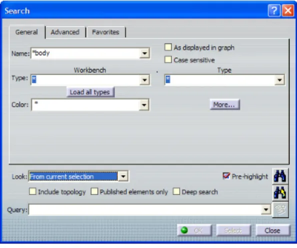
To view materials select “Shading with Material” on the “View” toolbar at the bottom of the screen. Highlight all the columns in the model tree. Go to the Search window

(Ctrl + F) and type “*body” in the “Name” field. Choose

“From current select” under the “Look” drop down menu. Click “Search and Select”.

1.

Now that you have the “Structural Solid Body” highlighted in each column click “Apply Material”. Choose the “Metal” tab, select “Steel” and press “Apply Material” and “Close”. You can repeat the previous steps for beams and apply

“Brushed metal 2” instead of “Steel” from the material

library.

2.

Select walls and type “envelope body” instead of “*body”

and apply “Wall of Castle” under the “Construction” tab in the material library. Expand the roof slab “Slab.1” and

select “Structural Solid Body”. Apply “Ox B&W Stripes”

under the “Other” tab in the material library. “Close” the material library after applying material.

3.

Material textures can give your model a more realistic appearance. Materials should be applied to Part Bodies with the building ele-ments.

Expand the “Structural Solid Body” under “Slab.1” and

select “Ox B&W Stripes”. A compass will appear in green at the model space 0,0. Grab an edge of the compass to

move or rotate the texture mapped in relationship to the roof slab.

4.

(30)

Parametric Change

Scroll up to the top of the model tree and double click “Sketch.1” inside of “Geometrical Set.1” to edit building boundary sketch. If geometrical set is hidden then unhide it to see sketch. Double click angle dimension to edit and change 15 degrees to 45. Click the “Exit workbench” but-ton to exit sketch. Wait for model to update.

1.

Double click “Plane.1” to edit the roof peak. Change the

offset height from 24’ to 48’ and click OK. Updating may take several minutes. Double click the “Line.2” object and change “End” to 36’. The roof will appear narrow with high

peaks in the front and back.

2.

From the changes just made, any number of building

ele-ments were automatically altered including wall location & height, column location & height, beam orientation and steel

end connections. Bundled within a single parameter change were countless changes to the building elements all follow-ing the dimensional rules originally set.

3.

All the building elements are implicitly connected to the “driving” geometry created in the initial steps. Changing a single parameter ripples changes throughout the model.

Continue exploring options for altering the configuration

of your project. If the model appears in red or indicates an update error then you have surpassed the limits of the model’s current rules. With more experience it is always

possible to change the rules to fit any number of extreme configurations.

4.

digital project V1,R4 Quick Start

Q u i c k S t a r t

digital

Quick Starting Your Knowledge in

Digital Project™ V1,R4

Table of Contents

Model Building Steps

Introduction

Creating a Part

Drawing the Building Outline

Drawing the Building Outline

Defining an Elevation Grid

Creating a Roof Slab

Inserting the Partition Sketch

Creating a Ground Floor Slab

Creating Exterior Walls

Inserting Doors

Placing Windows

Defining the Plan Grid

Creating Beams

Creating Beams

Adding Sloped Walls

Creating Columns

Generating Schedules

Creating a Drawing Sheet

Generating Drawings

Generating Drawings

Adding Drawing Annotations

Adding Drawing Annotations

Adding Materials

Parametric Change