NONPARAMETRIC BAYESIAN INFERENCES ON
PREDICTOR-DEPENDENT RESPONSE
DISTRIBUTIONS
by
Yeonseung Chung
A dissertation submitted to the faculty of the University of North Carolina at Chapel Hill in partial fulfillment of the requirements for the degree of Doctor of Philosophy in the Department of Biostatistics, School of Public Health.
Chapel Hill 2008
Approved by:
ABSTRACT
YEONSEUNG CHUNG: Nonparametric Bayesian Inferences on Predictor-Dependent Response Distributions.
(Under the direction of Dr. David Dunson.)
A common statistical problem in biomedical research is to characterize the relationship be-tween a response and predictors. The heterogeneity among subjects causes the response distri-bution to change across the predictor space in distridistri-butional characteristics such as skewness, quantiles and residual variation. In such settings, it would be appealing to model the condi-tional response distributions as flexibly changing across the predictors while conducting variable selection to identify important predictors both locally (within some local regions) and globally (across the entire range of the predictor space) for the response distribution change.
Nonparametric Bayes methods have been very useful for flexible modeling where nonpara-metric distributions are assumed unknown and assigned priors such as the Dirichlet process (DP). In recent years, there has been a growing interest in extending the DP to a prior model for predictor-dependent unknown distributions, so that the extended priors are applied to flexible conditional distribution modeling. However, for most of the proposed extensions, construction is not simple and computation can be quite difficult. In addition, literature has been focused on estimation and few attempts have been made to address related hypothesis testing problems such as variable selection.
Paper 1 proposes a local Dirichlet process (lDP) as a generalization of the Dirichlet pro-cess to provide a prior distribution for a collection of random probability measures indexed by predictors. The lDP involves a simple construction, results in a marginal Dirichlet process prior for the random measure at any specific predictor value, and leads to a straightforward posterior computation. In paper 2, we propose a more general approach not only estimating the conditional response distribution but also identifying important predictors for the response
ACKNOWLEDGMENTS
Though my name solely appears on the cover of this dissertation, many people have contributed to its production. I owe my gratitude to all those people who have made this dissertation possible, making my graduate experience one that I will cherish forever.
I would like to express my deepest appreciation to my advisor, Dr. David Dunson, with-out whom this dissertation would not have been possible. David continually and convincingly conveyed a spirit of adventure towards research, even as I struggled to face many unexpected hurdles. I will never forget his patient and endless support that helped me overcome many crises and his willingness to walk with me throughout my journey. His words of encouragement, quiet urgings and careful editing of my writing will never be forgotten. Besides David, I would also like to thank my committee members, Dr. Amy Herring, Dr. Donglin Zeng, Dr. Young Thruong, and Dr. Jiu-Chiuan Chen for their insightful comments and constructive criticisms.
In addition to my academic mentors, many friends have helped me remain strong through these difficult years. Their care and support have helped me overcome setbacks and stay focused on my graduate study. I am especially grateful for the support of one of my best friends, Jayeon Jeong, and to my faith family at First Korean Baptist Church.
I also appreciate the financial support from the National Institute of Environmental Health and Sciences that funded my doctoral research.
Most importantly, this dissertation would not have been possible without the love and pa-tience of my family. My family, to whom this dissertation is dedicated, has been a constant source of love, concern, support and strength. I cannot express enough my heart-felt gratitude for my family.
CONTENTS
LIST OF FIGURES x
1 INTRODUCTION 1
2 LITERATURE REVIEW 5
2.1 The Dirichlet Process (DP) . . . 5
2.1.1 Definition . . . 5
2.1.2 Polya urn scheme . . . 7
2.1.3 Stick-breaking representation . . . 8
2.1.4 Dirichlet process mixture (DPM) . . . 9
2.1.5 Posterior computation for DPMs . . . 9
2.2 DP-Extended Priors for Dependent Probability Measures . . . 11
2.2.1 Dependent Dirichlet process (DDP) and its variations . . . 11
2.2.2 Convex combinations of DPs . . . 14
2.3 Nonparametric Bayes Estimation for Predictor-Dependent Response Distributions 17 2.3.1 DPM of regressions and its predictor-dependent extension . . . 17
2.3.2 DPM for the joint distribution of response and predictors . . . 19
2.4 Nonparametric Bayes Hypothesis Testing in Predictor-Dependent Response Dis-tributions . . . 19
2.4.1 Model selection . . . 20
2.4.2 Testing for distributional changes . . . 21
3 THE LOCAL DIRICHLET PROCESS (LDP) 23
3.1 Introduction . . . 23
3.2 Predictor-Dependent Stick-Breaking Priors . . . 26
3.2.1 Stick-Breaking Priors . . . 26
3.2.2 Predictor-Dependent Stick-Breaking Priors . . . 26
3.3 Local Dirichlet Process . . . 27
3.3.1 Formulation . . . 27
3.3.2 Moments and Correlation . . . 31
3.3.3 Truncation Approximation . . . 33
3.4 Posterior Computation . . . 36
3.5 Simulation Examples . . . 39
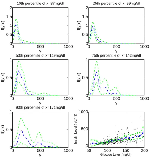
3.6 Epidemiological Application . . . 43
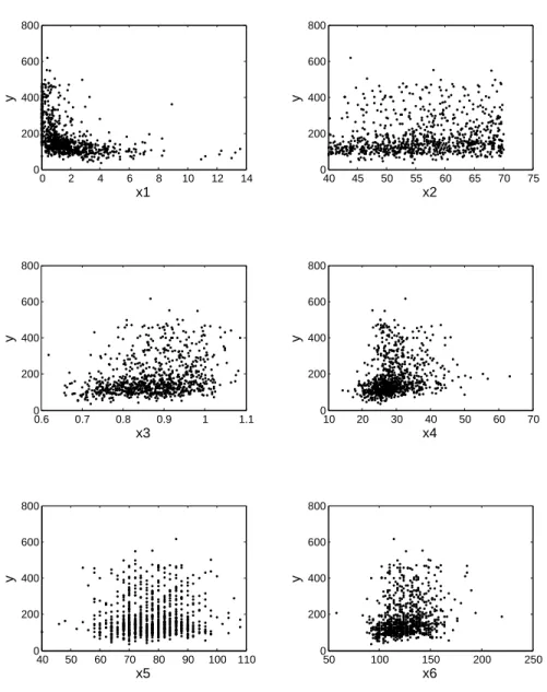
3.6.1 Background and Motivation . . . 43
3.6.2 Analysis and Results . . . 43
3.7 Discussion . . . 45
4 NONPARAMETRIC BAYES CONDITIONAL DISTRIBUTION MODEL-ING WITH VARIABLE SELECTION 47 4.1 Introduction . . . 47
4.2 The Probit Stick-Breaking Process . . . 50
4.2.1 Formulation . . . 50
4.2.2 Moments . . . 52
4.3 Conditional Distribution Modeling With Variable Selection . . . 54
4.3.1 Model Specification . . . 54
4.3.2 Hypothesis Formulation . . . 56
4.5 Simulation Study . . . 60
4.5.1 Simple Application of PSBPM . . . 61
4.5.2 Comparison with a simple and a competing method . . . 63
4.6 Epidemiological Application . . . 66
4.6.1 Motivation and Background . . . 66
4.6.2 Analysis . . . 68
4.7 Discussion . . . 70
5 BAYES VARIABLE SELECTION IN LATENT CLASS MODELING OF LONGITUDINAL DATA 71 5.1 Introduction . . . 71
5.2 Mixture Models for Longitudinal Data with Variable Selection . . . 74
5.2.1 Predictor-Dependent Mixture Model . . . 74
5.2.2 Variable Selection and Hypothesis Testing . . . 76
5.3 Posterior Computation . . . 77
5.3.1 MCMC algorithm . . . 77
5.3.2 Default Choices for Hyperparameters . . . 78
5.4 Simulation Study . . . 79
6 CONCLUDING REMARKS AND FUTURE RESEARCH 84
Appendix
88
A Proofs in Chapter 3 88
B Proofs in Chapter 4 91
C Proofs in Chapter 5 95
REFERENCES 98
LIST OF FIGURES
3.1 Graphical illustration for lDP formulation . . . 29
3.2 Change in correlation . . . 34
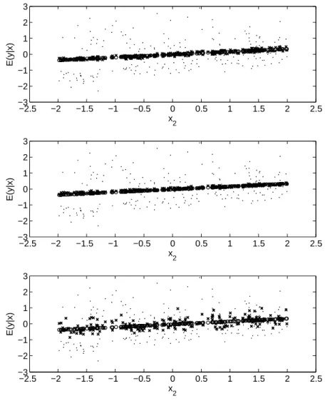
3.3 Results for simulation case 1 . . . 41
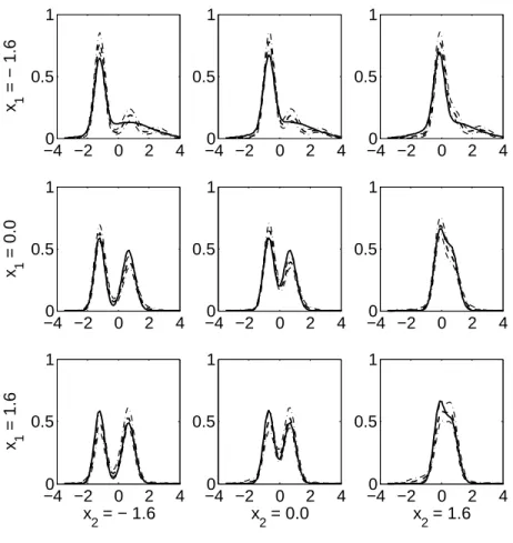
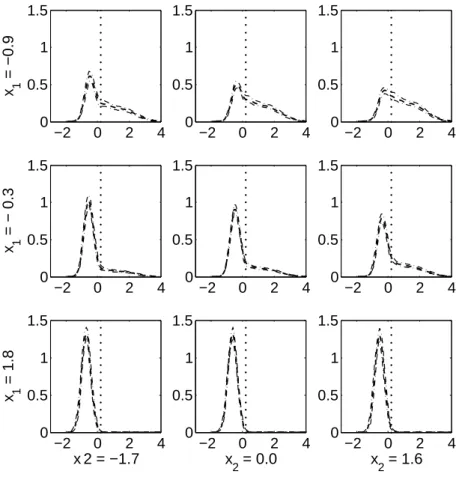
3.4 Results for simulation case 2 . . . 42
3.5 Results for Pima indian data example . . . 44
4.1 Posterior probabilities for null hypothesis in simulation 3 . . . 62
4.2 Predictive density for simulation 3 . . . 63
4.3 Prediction performance comparison . . . 65
4.4 Data from IRAS study . . . 67
4.5 Predictive density for IRAS study . . . 69
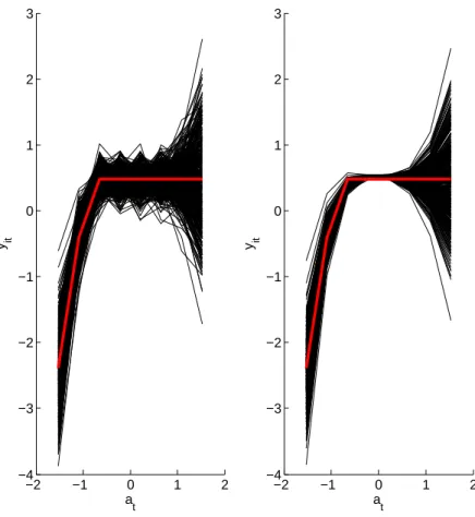
5.1 Case (1) . . . 81
5.2 Case (2) . . . 82
CHAPTER 1
INTRODUCTION
flexible characterization of predictor-dependent response distributions, one may fit DPM models separately for different predictor levels, which results in smooth estimation of predictor-specific response distributions. However, the approach of fitting several DPM models at different pre-dictor levels is disadvantageous in that it neither models trends nor borrows information across the predictor space, which is particularly important in applications having a modest number of subjects. In addition, the approach requires some arbitrary categorization for continuous predictors, which can discard valuable information. Furthermore, as the number of predictor categories increases, estimation and testing efficiency may decrease.
In recent years, there has been a growing interest in extending the DP to a prior model for predictor-dependent unknown probability measures. Most of this literature has relied on extend-ing the stick-breakextend-ing representation of the DP (Sethuraman, 1994) and has been stimulated by the dependent Dirichlet process (DDP) framework proposed by MacEachern (1999, 2000, 2001), which replaces the atoms in the stick-breaking representation of the DP with stochastic pro-cesses. The DDP structure has been adopted to develop ANOVA-type dependence for random probability measures (De Iorio et al., 2004), for flexible spatial modeling (Gelfand et al., 2004), and for inferences on stochastic ordering (Dunson and Peddada, 2008). The specification of the DDP used in applications incorporates dependence only through the atoms while assuming fixed weights. In other recent work, Griffin and Steel (2006; 2008) proposed an order-based DDP (πDDP) which allows varying weights, while Duan et al. (2005) developed a multivariate stick-breaking process for spatial data. In addition, Teh et al. (2004) proposed the hierarchi-cal Dirichlet process (hDP) which generates group-specific random probability measures having group-dependent weights but sharing atoms in their stick-breaking forms.
time data. In addition, Rodriguez et al. (2008) used DP-type combination of DPs called nested DP (nDP) which was motivated by the idea of clustering groups and subjects within a group simultaneously. Recently, the idea has been extended to continuous covariate cases by Dunson et al. (2007) and Dunson and Park (2008).
However, for most of the DP-extended priors discussed so far, they are limited either to the cases of categorical predictors or, for continuous predictor cases, to complicated computation causing the methods to be unaccessible in many applications. In addition, this literature has been focused on estimation and few attempts have been made to address related hypothesis testing problems such as variable selection or detecting distributional changes both globally (across the entire predictor space) and locally (within some local predictor regions). In fact, there has been limited focus on hypothesis testing and model selection in Bayesian nonparametric literature. Basu and Chib (2003) proposed an approach for calculating marginal likelihoods and Bayes factors for comparing DPM models. But this approach is not directly applicable to our local variable selection problem. Pennell and Dunson (2008) proposed a method for testing distributional changes in response across an ordinal predictor while Dunson and Pedadda (2008) tested equalities in group specific response distributions against a stochastic ordering. Both approaches deal with a categorical predictor whereas we seek for a methodology that can incorporate a mix of continuous predictors as well as categorical predictors.
Motivated by this, paper 1 proposes a local Dirichlet process (lDP) as a generalization of the Dirichlet process to provide a prior distribution for a collection of random probability measures indexed by predictors. The lDP should be useful to other alternative prior models for dependent random probability measures in that it involves a simple construction, results in a marginal Dirichlet process prior for the random measure at any specific predictor value, and leads to a straightforward posterior computation. Theoretical properties are considered and a blocked Gibbs sampler is proposed for posterior computation in lDP mixture models. The methods are illustrated in a conditional distribution modeling setting using simulated examples and an epidemiologic application.
In paper 2, we propose a more general approach for conditional distribution modeling where
we not only estimate the conditional response distribution addressing the distributional changes across the predictor space, but also identify important predictors for the response distribution change both with local regions and globally. We first introduce the probit stick-breaking process (PSBP) as a prior for an uncountable collection of predictor-dependent random probability measures and propose a PSBP mixture (PSBPM) of normal linear regressions. A global variable selection structure is incorporated to drop unimportant predictors out from the model using the posterior inclusion probabilities. Local variable selection is conducted relying on the conditional distribution estimates at different predictor points. An efficient stochastic search sampling algorithm is proposed for posterior computation. The methods are illustrated through simulation and applied to an epidemiologic study.
CHAPTER 2
LITERATURE REVIEW
This chapter consists of literature review for: (1) the Dirichlet process (DP) as a prior model for a random probability measure, (2) various extensions of the DP as a prior model for a collection of predictor-dependent probability measures, (3) nonparametric Bayes estimation for predictor-dependent response distributions, (4) nonparametric Bayes hypothesis testing in predictor-dependent response distributions.
2.1
The Dirichlet Process (DP)
Bayesian inference involves placing distributions over variables in a statistical model. More flexibly, one can place a prior distribution over the space of distributions. The Dirichlet process (DP) is a popularly used prior model for an unknown distribution. In this section, the literature about the DP and its important properties are reviewed.
2.1.1
Definition
given by
P(p|α, M) = Qk Γ(α)
i=1Γ(αmi)
k Y
i=1
pαmi−1
i , (2.1)
whereM ={m1, . . . , mk} is the mean value of p and α is a precision parameter that says how
concentrated the distribution is around M. Both M and p sum to unity. α can be regarded as the number of pseudo-measurements observed to obtain M. The greater the number of pseudo-measurements is, the more our confidence inM is, and hence, the more the distribution is concentrated around M.
The Dirichlet distribution defines a distribution over a space of discrete distributions. Let p={p1, . . . , pk}be a probability distribution on the discrete spaceX ={X1, . . . ,Xk}such that
P(X =Xi) =pi, where X is a random variable in the space X. Sampling a Dirichlet from (2.1)
results in a distributionpon the discrete spaceX. The Dirichlet distribution defined on a space of discrete probability measures onX can be noted as:
p(X1), . . . ,p(Xk)∼Dirichlet(αm1, . . . , αmk) (2.2)
If we consider a continuous sample space Θ and its disjoint partition such as Θ =∪k
i=1Bi, it is
apparent that a Dirichlet distribution exists on every disjoint partition of a continuous space Θ because the partition{B1, . . . , Bk}is itself a discrete space.
Now consider a probability space (Θ,B, G), where Θ ⊂ <d, B corresponds to the Borel
σ-algebra of subsets of <d, and G is a probability measure on (Θ,B). Also, consider
an-other probability space (G,C,P), where G is the space of probability measures G defined on (Θ,B) and C is the corresponding σ-algebra. Then, the DP with base measure G0 and
preci-sion α, denoted as DP(αG0), is a measure P defined on (G,C) such that G(B1), . . . , G(Bk) ∼
2.1.2
Polya urn scheme
The formal definition of the DP described in the previous section does not lend itself to an understanding of its distributional property. One way of understanding the DP more intuitively is connecting it to the Polya urn scheme (Blackwell and MacQueen, 1973; Escobar, 1994).
Consider an urn with α balls, of which initially αmj are of color j, 1≤j ≤k (assuming for
now that all the αmj are integers). We draw balls at random from the urn, replacing each ball
by two balls of the same color. Let Xi =j if the ith ball is of color j. Then,
p(X1 =j) =
αmj
α
p(X2 =j|X1) =
αmj+ 1(X1 =j)
α+ 1 ..
.
p(Xn =j|X1, . . . , Xn−1) =
αmj+Pn
−1
k=11(Xk=j)
α+n−1 (2.3)
We call this sequenceX1, . . . , Xn as a Polya urn sequence.
Let φi be ith sample from G with G ∼ DP(αG0). Then, it was shown that marginalizing
overG, φi is generated according to the following sequence:
φ1 ∼ G0
φ2|φ1 ∼
αG0+δφ1
α+ 1 ..
.
φn|φ1, . . . , φn−1 ∼
αG0+Pn
−1
k=1δφk
α+n−1 , (2.4)
whereδφi is a degenerate measure concentrated at φi. The sequence in (2.4) can be viewed as a
Polya urn sequence by considering the limit as the number of colors in the Polya urn tends to a continuum. We call (2.4) the Polya urn scheme for the marginal distribution of a sample φi
from a random probability measureG following a DP(αG0).
The Polya urn scheme of the DP results in a clustering structure amongstφ1, . . . , φnwith the
following conditional distribution of eachφi, givenφ(i) ={φ1, . . . , φi−1, φi+1, . . . , φn}
(MacEach-ern, 1994; West et al., 1994).
φi|φ(i) ∼
α α+n−1
G0 +
1
α+n−1
k(i) X
j=1
n(ji)δθ(i)
j
, (2.5)
where φ(i) takes on k(i) distinct values that are θ(i)
j for j = 1, . . . , k(i), and n
(i)
j is the number
of samples takingθ(ji) in φ(i). Similarly, the predictive distribution of a future φi for i =n+ 1
givenφ={φ1, . . . , φn} follows:
φn+1|φ∼
α α+n
G0+
1
α+n
k
X
j=1
njδθj, (2.6)
whereφ takes on k distinct values that areθj forj = 1, . . . , k, and nj is the number of samples
taking θj in φ.
2.1.3
Stick-breaking representation
An important representation of the DP is the stick-breaking representation constructed by Sethuraman (1994). The random probability measureGsampled from a DP(αG0) is represented
as:
G= ∞
X
h=1
phδθh, (2.7)
where ph = VhQh
−1
l=1(1 − Vl) with Vh
iid
∼ Beta(1, α) and θh iid
∼ G0 for h = 1, . . . ,∞. The
ph are called stick-breaking random weights and θh called random atoms. It was shown that P∞
h=1ph ≈ 1 almost surely to ensure G is an appropriate probability measure. This
measures (reviewed in section 2.2.1).
2.1.4
Dirichlet process mixture (DPM)
The DP generates a random distribution that is almost surely discrete, which is problematic in modeling a continuous distribution. A simple solution to this problem is to use a Dirichlet process mixture (DPM) (Lo, 1984; Escobar, 1994; Escobar and West, 1995). Let yi be ith
subject’s response following a continuous distribution F with unknown parameter φi, where φi
follows an unknown probability measureG. By placing a DP prior forG, we model the marginal distributionF as a DPM model ensuring thatyihas a continuous distribution while still relaxing
the distributional assumptions. The hierarchical structure of the DPM model is expressed as:
yi|φi ∼ F(·;φi)
φi|G ∼ G(·)
G|α,ψ ∼ DP(αG0(·;ψ)), (2.8)
whereψ are the parameters of the parametric distribution G0.
In recent years, with the availability of simple and efficient methods for posterior compu-tation (see section 2.1.5), the DPM model has been widely used in many applications, which include finance (Kacperczyk et al., 2003), econometrics (Chib and Hamilton, 2002), epidemi-ology (Dunson, 2005), genomics (Xing et al., 2004; Kim et al., 2007), medicine (Kottas et al., 2002; Bigelow and Dunson, 2008), and machine learning (Beal et al., 2002 and Blei et al., 2004).
2.1.5
Posterior computation for DPMs
Analytic derivation of the posterior distributions for random quantities of interest is prohib-ited for the DPM models. Much of the DPM literature has been devoted to develop the Markov chain Monte Carlo (MCMC) techniques which allow sampling-based posterior inference in the DPM models.
There are two possible approaches in the MCMC techniques for the DPM models. The first one, called the marginal method, was introduced by Escobar (1994) and Escobar and West (1995), and has been substantially improved in MacEachern (1994), M¨uller et al. (1996) and par-ticularly in MacEachern and M¨uller (1998) and Neal (2000). The marginal approach integrates out the random distribution G over the DP prior and uses convenient Polya urn representa-tion within a Gibbs sampler to obtain posterior samples. Although simple to implement, this marginal method has a main drawback that a single-component updating Gibbs sampler is used to sample from a multivariate distribution of dependent variables, which results in problems in moving clusters around the posterior space, and therefore the mixing can be very slow even for moderately sized data sets. To improve the slow mixing problem, several MCMC samplers have been recently proposed based on the split-merge moves. Green and Richardson (2001) proposed one based on the reversible-jump procedure in which numerous ways to propose the split move are possible. Jain and Neal (2004) introduced a Metropolis-Hastings technique with split-merge proposals for conjugate DPM models and the idea was extended to a non-conjugate cases (Jain and Neal, 2007). Dahl (2003) suggested a sequentially-allocated split-merge sampler (SAMS) as an alternative to Jain and Neal (2004) approach.
Another MCMC tool, called the conditional approach or blocked Gibbs sampler, has been advocated by Ishwaran and Zarepour (2000) and Ishwaran and James (2001), who found that it can lead to considerably more robust convergence properties than the marginal approach. The conditional method, instead of integrating it out, augments the random distribution G
error depending on the truncation accuracy. Avoiding such approximation, Papaspiliopoulos and Roberts (2004) designed an MCMC algorithm which samples from the exact posterior dis-tribution of all quantities of interest based on the technique of retrospective sampling. More recently, Walker (2007) proposed slice sampling idea which avoids both marginalization and truncation.
Alternatively to the MCMC methods, other techniques for posterior inference in the DPM models have been proposed. This literature include sequential importance sampling (MacEach-ern et al., 1999) and variational methods (Blei and Jordan, 2006).
2.2
DP-Extended Priors for Dependent Probability
Mea-sures
The DP is a prior model for an unknown probability measure. However, modeling the rela-tionship between predictors and the unknown probability measures cannot be achieved directly using the DP. In this section, the work for developing prior models for predictor-dependent unknown probability measures is reviewed.
2.2.1
Dependent Dirichlet process (DDP) and its variations
MacEachern (1999, 2000, 2001) proposed the dependent Dirichlet process (DDP) as a prior model for dependent distributions. Consider a collection of predictor-dependent random mea-sures GX = {Gx : x ∈ X }, where X is a predictor space. The DDP defines a probability distribution Gx for each x as Gx =
P
phδθxh, where ph are stick-breaking random weights as
in a DP and θxh are predictor-dependent random atoms. In the ”single-p DDP”, a special case
of the DDP, the weights ph are common to allGx while the dependence is induced acrossx by assuming that θh ={θxh : x ∈ X } are iid realizations of a stochastic process in x (e.g.
Gaus-sian process). Independence across h, together with the stick-breaking weights ph, guarantees
that Gx marginally follows a DP. Dependence in the sample path of the stochastic process θh
introduces the desired dependence acrossx.
De Iorio et al. (2004) used the DDP structure to develop an ANOVA-like probability model over a collection of random distributions. They considered a categorical predictorx, which, for simplicity of explanation, is bivariate as x = (v, w)0 with v ∈ {1, . . . , V} and w ∈ {1, . . . , W}. Using the DDP framework to induce an ANOVA-type dependence among Gx, they defined
Gx =
P
phδθxh, where θxh =mh +Avh+Bwh with mh iid
∼G0
m, Avh iid
∼ G0
Av, and Bwh iid
∼ G0
Bw for
v = 1, . . . , V andw= 1, . . . , W. They referred to this probability model as ANOVA-DDP(α, G0)
whereG0 = (G0
m,{G0Av}Vv=1,{G0Bw}Ww=1).
Gelfand et al. (2005) applied the DDP framework to develop a spatial DP process (SDP) model for spatial data. They considered a point-referenced spatial data assumed to arise as a sample from a realization of a random field (random process) YD = {Y(s) : s ∈ D} with
D⊂ <d. Simply using the DDP idea, Y
D was modeled as a random spatial process denoted by P∞
h=1phδθh,D, where ph are the stick-breaking weights as in DP and θh,D ={θh(s) : s ∈D} is
a stochastic process G0 over the D. Letting s(n) = (s1, . . . , sn) be a specific distinct locations
inD where the observations are collected, the full data set consists of the collection of vectors
Y ={Y(s1), . . . , Y(sn)}. Then, the SDP induces a random probability measureG(n)on the space
of distribution functions forY asG(n)∼DP(αG0(n)), where G(0n) is an n-variate distribution for
Y induced by G0. With the joint distribution using the same set of stick-breaking weights for
any group of n locations, the SDP results in the common surface selection for all locations in the group.
The DDP structure also has been used by Dunson and Peddada (2008) to propose restricted dependent Dirichlet process (rDDP) which has a full support in the space of stochastically ordered random distributions. They considered a collection of probability measures{P1, . . . , Pk}
that belongs to the following convex subset of PK:
is a partial ordering. Here, Pi Pj denotes that Pj is stochastically larger than Pi such as
Pi(x,∞)≤Pj(x,∞) for allx. As a prior for (P1, . . . , PK)∈CE, the proposed rDDP defines Pk
as:
Pk =
∞
X
h=1
phδθhk, ph =Vh Y
l<h
(1−Vl), k= 1, . . . , K, (2.10)
whereph are stick-breaking weights withVh iid
∼Beta(1, α) andθh = (θh1, . . . , θhK)0 iid
∼ P0 are
ran-dom atoms. Here,P0 is a Borel probability measure defined onSE, where SE ={(s1, . . . , sK)∈
XK :s
i ≤sj ∀(i, j)∈E}.
Relaxing the fixed weight assumption in the DDP framework used so far, Griffin and Steel (2006) proposed an ordered DDP (πDDP) which results in predictor-dependent weights as well as predictor-dependent atoms. For a collection of predictor-dependent random distributions, GX, the πDDP defines Gx as:
Gx =
n(x)
X
l=1
pl(x)δθπl(x), pl(x) = Vπl(x) Y
j<l
(1−Vπj(x)), ∀x∈ X (2.11)
where θh iid
∼ G0, Vh iid
∼ Beta(1, α), for h = 1, . . . ,∞, and π(x) = {π1(x), . . . , πn(x)(x)} is an
ordering for the stick-breaking construction ofGx at the predictor pointx, which is assigned an ordering process{π(x) :x∈ X }.
Duan et al. (2006) also relaxed the fixed weight assumption in the Gelfand et al. (2005) SDP and proposed a generalized SDP (GSDP) as a multivariate generalization of the stick-breaking prior, which enables different surfaces to be assumed at different locations. The GSDP generates a spatial process for YD such that, for any set of locations s(n) ∈D,
Y(s1), . . . , Y(sn)∼
∞
X
i1=1
. . .
∞
X
in=1
pi1,...,inδθi∗1(s1), . . . , δθ∗in(sn), (2.12)
where theθ∗j are independent and identically distributed asG0,ij is an abbreviation fori(sj), j =
1,2, . . . , n, and the weights{pi1,...,in}, conditionally on the locations, have a distribution defined
on the infinite dimensional simplex:
P={pi1,...,in ≥0 :
∞
X
i1=1
. . .
∞
X
in=1
pi1,...,in = 1}. (2.13)
Another relevant extension of the DP is the hierarchical Dirichlet process (hDP) proposed by Teh et al. (2004). The hDP generates group-specific random distributionsGj from a DP(αG0),
where G0 is drawn from another DP(γH). The fact that G0 is discrete ensures that Gj are
dependent across different groups through sharing the atoms. The stick-breaking forms of G0
and Gj are more informative of this dependence structure as:
G0 =
∞
X
h=1
βhδθh, Gj =
∞
X
h=1
pjhδθh, (2.14)
whereβh andθh are random stick-breaking weights and atoms from DP(γH) andpjh are
group-dependent random weights constructed based on the random weightsβh of DP(γH) and ph of
DP(α, G0). This can be viewed as the case of group-dependent weights with fixed atoms in the
DDP framework.
2.2.2
Convex combinations of DPs
A different approach that has been used for developing prior models inducing predictor-dependence is using linear combinations of realizations of Dirichlet process(es). M¨uller et al. (2004) proposed a prior model for k experiment-dependent distributions as a linear combina-tion of one global component G∗0 and k experiment-specific innovation measures G∗1, . . . , G∗k, with all G∗h assigned independent DP(αh, G0h), for h = 0, . . . , k. The hth experiment-specific
distribution is expressed asGh =πG∗0+ (1−π)G
∗
h.
distributions as:
G1 ∼ DP(α0G0)
G2 = (1−π1)G1+π1G∗1,
.. .
Gh = (1−πh−1)Gh−1+πh−1G∗h−1
= wh1G1+
h−1
X
l=1
wh,l+1G∗l (2.15)
whereG∗1 ∼DP(α1G01),G∗l ind
∼ DP(αlG0l) forl = 1, . . . , h−1, 0≤πl≤1,whl =πl−1
Qh−1
m=1(1−
πm) for l = 1, . . . , h−1 and whl =πh−1 for l =h with π0 = 1, G∗l are innovation distributions
that characterize changes in the distribution caused by increasing the predictor level from l to
l+ 1, and G0l are known distributions. As we move from predictor level from l to l + 1, we
decrease the weights assigned toG1, G∗1, . . . , G∗l−1 and introduce a new unknown distribution to
our mixture, G∗l. This evolution in Gh is reasonable in a situation where as the predictor level
increases, more changes in the response distribution are expected.
Rodriguez et al. (2008) proposed another type of linear combination of DP realizations, called nested Dirichlet process (nDP), which defineshth group-dependent random distribution as Gh = P
∞
l=1π
∗
lG∗l ,where π∗l = v∗l Ql−1
j=1(1−v
∗
j) with vj∗ iid
∼ Beta(1, α), and G∗l iid∼ DP(βG0).
The i.i.d. realizations of aDP(βG0),G∗l, are linearly combined with another DP stick-breaking
weightsπl∗. When the nDP is considered as a prior for group-dependent mixture distributions in a mixture model, it induces clustering predictor groups while identifying clusters of subjects within each predictor group.
While the above three prior models were for a categorical predictor case, similar idea was used for a continuous predictor case. Dunson et al. (2006) proposed a weighted mixture of DPs (WMDP) which defines a random distribution at a particular predictor pointx as:
Gx=
n X
j=1
bj(x)G∗xj, G
∗ xj
iid
∼DP(αG0), for j = 1, . . . , n, ∀x∈ X, (2.16)
where b(x) = (b1(x), . . . , bn(x))0 is a predictor-dependent weight function mapping from X →
Pn, with Pn being the n-dimensional probability simplex, so that bj(x) ≥ 0, j = 1, . . . , n,
and b(x)01n = 1, for all x ∈ X. The collection GX∗ = {G ∗
xi;i = 1, . . . , n} consists of i.i.d.
realizations from a DP(αG0) indexed by sampled predictor values xi. Hence, the WMDP for
GX = {Gx;x ∈ X } is defined by placing a DP-distributed basis random measures at each of the sample predictor values, and then mixing across these basis measures to construct an uncountable collection of random probability measures for all possible predictor valuesx ∈ X. For the weight function b(x), they used a kernel-based weighting scheme such as:
bj(x) =
γjK(x,xj) Pn
l=1γlK(x,xl)
, j = 1, . . . , n, ∀x∈ X, (2.17)
whereγ = (γ1, . . . , γn)0 represent weights on the differentbasislocations, andK :X × X → <+
is a kernel function, such asK(x,x0) = exp(−ψ||x−x0||2).
Avoiding the sample dependence of the WMDP, which is problematic from a Bayesian per-spective and results in some unappealing properties, Dunson and Park (2008) proposed a class of kernel stick-breaking process (KSBP) to be used as a sample-free prior for GX, which induces a predictor-dependent prediction rule upon marginalization. The KSBP defines Gx as:
Gx = ∞
X
h=1
Ph(x)G∗h,
Ph(x) = W(x;Vh,Γh) Y
l<h
1−W(x;Vl,Γl)
W(x;Vh,Γh) = VhK(x,Γh), ∀x∈ X, (2.18)
where Γh iid
∼ H are random locations, Vh ind
∼ beta(ah, bh) are probability weights, and G∗h iid
∼ Q
are probability measures, for h = 1, . . . ,∞. Here, H is a probability measure defined on X0 which may or may not correspond to X, Q is a probability measure on a space of probability
Bases located close to x and having a smaller index, h, will tend to receive higher probability weight. In this manner, the KSBP accommodates dependence betweenGx and Gx0.
2.3
Nonparametric Bayes Estimation for Predictor-Dependent
Response Distributions
Recall that our goal is to flexibly characterize the relationship between a responsey∈ Y and predictors x = (x1, . . . , xp)0 ∈ X. The challenge is that a parametric form for the conditional
distribution of y given x is unknown and the changes in the distributional shape needs to be addressed across the predictors x. In this section, nonparametric Bayes methods for flexible conditional distribution modeling are reviewed.
2.3.1
DPM of regressions and its predictor-dependent extension
It is well known that a mixture of a sufficiently-large number of normal densities can ap-proximate any smooth density. For a flexible characterization of the conditional density of a response given predictors, one can consider the following mixture of regression models:
f(yi|xi) = Z
f(yi|xi, φi)dGxi(φi), (2.19)
where f(yi|xi, φi) = N(yi;x0iβi, σi2), with φi = (βi, σi2). Depending on the choice of Gxi, the
model (2.19) encompasses a wide variety of flexible regression models as special cases including normal linear regression, linear regression with the residual density modeled as a finite/infinite mixture of normals, and a finite/infinite mixture of regressions.
In nonparametric Bayes methods, one choice ofGxi is such thatGxi ≡Gis assumed unknown
and assigned a DP(αG0) prior, under which the model (2.19) becomes an infinite mixture of
regressions as:
f(yi|xi) =
∞
X
h=1
phN(yi;xi0βh, σh2), (2.20)
where ph are an infinite sequence of random stick-breaking weights and (βh, σ2h) are random
atoms i.i.d. sampled from G0. The DPM of regressions in (2.20) is relatively flexible in that it
incorporates an infinite number of normal linear regression components with a few components having most of the weights depending on the precision prior α, particularly when the number of mixture components is uncertain. However, assuming that the weights ph are constant across
the predictors still restricts the conditional density in that the shape of residual variation is the same across the predictors and the mean regression structure is linear as:
E(yi|xi) =
∞
X
h=1
phx0iβh =
∞
X
h=1
ph p X
j=1
xijβhj = p X
j=1
xij
∞
X
h=1
phβhj =x0iβ¯, (2.21)
where ¯β =P∞
h=1phβhj.
Applying the prior models for a collection of predictor-dependent random distributions, the assumptionGxi ≡Gin the DPM of regression model can be relaxed. As reviewed in section 2.2,
any prior model P for GX ={Gxi xi ∈ X } can be incorporated in the mixture model specified
in (2.19) as:
f(yi|xi) = Z
f(yi|xi, φi)dGxi(φi),
GX = {Gxi xi ∈ X }, GX ∼ P, (2.22)
wheref(yi|xi, φi) =N(yi;x0iβi, σi2), with φi = (βi, σi2). Dunson et al. (2007), Griffin and Steel,
2.3.2
DPM for the joint distribution of response and predictors
Alternatively, instead of assuming that the predictors to be included are known, M¨uller et al. (1996) proposed a different approach for flexible characterization of the conditional density of response given predictors. The joint density of response and predictors was modeled as a DP normal mixture model, which leads to the conditional density as an infinite mixture of regression models, with the mixture weights varying with predictors. Let yi be ith subject’s response and
xi be ith subject’s predictors. For zi = (yi,x0i)
0, the DP normal mixture model is expressed as:
f(zi) = Z
N(zi;µzi,Σzi)dG(µzi,Σzi)
G ∼ DP(αG0) (2.23)
This leads tof(zi) = P
∞
h=1phN(zi;µ
∗
zh,Σ
∗
zh), which also leads to the conditional densityf(yi|xi)
as:
f(yi|xi) =
f(zi)
f(xi)
=
P∞
h=1phN(zi;µ∗zh,Σ
∗
zh) P∞
h=1phN(xi;µ
∗ xh,Σ
∗ xh)
=
P∞
h=1phN(yi;x0iβ
∗
h, σh∗2)N(xi;µ∗xh,Σ
∗ xh) P∞
h=1phN(xi;µ
∗ xh,Σ
∗ xh)
= ∞
X
h=1
ph(xi)N(yi;x0iβ
∗
h, σ
∗2
h ), (2.24)
which is an infinite mixture of regression models, with the mixture weights ph(xi) varying with
predictors, where ph(xi) =
phN(xi;µ∗xh,Σ
∗
xh)
P∞
h=1phN(xi;µ∗xh,Σ
∗
xh)
.
2.4
Nonparametric Bayes Hypothesis Testing in
Predictor-Dependent Response Distributions
A flexible characterization of the relationship between a response and predictors involves not only the estimation of the predictor-specific response distribution but also the hypothesis testing of the distributional changes across the predictors or for model selection through the
identification of significantly associated predictors both globally and locally. In this section, little work addressing the related problems is reviewed.
2.4.1
Model selection
Basu and Chib (2003) proposed an approach comparing semi-parametric models, constructed under the DPM framework, with alternative semi-parametric Bayesian models. They considered a model space {M1, . . . ,MJ}, where one (or more) of the models is a DPM model. Given a
data y = (y1, . . . ,yn), they suggested a formal Bayesian approach comparing any two models
Mr and Ms using the Bayes factor which is the ratio of marginal likelihoods as:
Brs=
m(y|Mr)
m(y|Ms)
(2.25)
2.4.2
Testing for distributional changes
Pennell and Dunson (2007) proposed a method for testing for distribution changes across an ordinal predictor. They considered the specific response distribution as predictor-dependent mixture model using the DMDP prior (Dunson, 2006) for the mixture distributions. The model is expressed as:
fh(yhi) = Z
N(yhi;µhi,Σhi)dGh(µhi,Σhi)
{G1, . . . , GK} ∼ DM DP(πl, αl, G0l, l= 1, . . . , K−1) (2.26)
Here, it is immediately apparent that differences in mixture distributions, Gh and Gh+1, imply
differences in the response distributions, fh and fh+1. Hence, the local null hypothesis was
defined with respect to the total variation (tv) distances between two mixture distributions of adjacent predictor levels as follows:
H0h :||Gh+1−Gh||T V ≤, for h= 1, . . . , K −1, (2.27)
where is some small constant such that when H0h holds, there is no appreciable difference in
the mixture distributions across groupshand h+ 1. It was shown that the tv distance between
Gh+1 and Gh is totally controlled by πh, so the local null can be equivalently stated as:
H0h :πh ≤∗, for h= 1, . . . , K−1, (2.28)
Placing a prior πh ∼ p0hUniform(0, ∗) + (1−p0h)Uniform(∗,1) for πh, for h = 1, . . . , K −1,
allowed for calculating the posterior probability for H0h. The global null of no changes in
response distribution across groups (H0) corresponds to the intersection of theses local nulls.
Furthermore, Dunson and Peddada (2008) proposed a method for testing equalities of distri-butions against stochastically ordered alternatives in the rDDP mixture model framework (Refer to the summary in section 2.2.2). For a two group problem where P1 P2, they considered
rDDP withP0 chosen as:
f(θ1,θ2) =f1(θ1){π0δ0(θ2−θ1) + (1−π0)f2(θ2−θ1)}, (2.29)
where X = <, f1(·) is a density on < (e.g. Gaussian), 0 ≤ π0 ≤ 1 is the prior probability of
θ1 =θ = 2, and f2(·) is a density with support on <+ (e.g. truncated Gaussian). To formally
assess how closeP1 and P2, they defined a distance metric as:
d12 = max
x∈X
P2(x,∞)−P1(x,∞)
(2.30)
and formulate the null hypothesis that P1 and P2 are close in some sense to an alternative of
stochastic ordering as:
H0 :d12≤ and d12> , (2.31)
where >0 is a small positive constant. The posterior probability for the null hypotheses were calculated based on the fact thatd12=P
∞
h=1ph1(βh >0)∼Beta(α(1−π0), απ0). The idea was
generalized to multiple group cases and the global null hypothesis was defined as:
H0 : ∪Kk=1−1H0k
CHAPTER 3
THE LOCAL DIRICHLET PROCESS
(LDP)
3.1
Introduction
In recent years, there has been a dramatic increase in applications of nonparametric Bayes methods, motivated largely by the availability of simple and efficient methods for posterior computation in Dirichlet process mixture (DPM) models (Lo, 1984; Escobar, 1994; Escobar and West, 1995). The DPM models incorporate Dirichlet process (DP) priors (Ferguson, 1973, 1974) for components in Bayesian hierarchical models, resulting in an extremely flexible class of models. Due to the flexibility and ease in implementation, DPM models are now routinely implemented in a wide variety of applications, ranging from machine learning (Beal et al., 2002 and Blei et al., 2004) to genomics (Xing et al., 2004 and Kim et al., 2006).
In many settings, it is natural to consider generalizations of the DP and DPM-based models to accommodate dependence. For example, one may be interested in studying changes in a density with predictors. Following Lo (1984), one can use a DPM for Bayes inference on a single density as follows:
f(y) =
Z
Ω
where k(y, u) is a non-negative valued kernel defined on (D ×Ω,F × B) such that for each
u ∈ Ω, RDk(y, u)dy = 1 and for each y ∈ D, R
Ωk(y, u)G(du) < ∞ with D,Ω Borel subsets
of Euclidean spaces and F,B the corresponding σ-fields, and G is a finite random probability measure on (Ω,B) following a DP. A natural extension for modeling of a conditional density
f(y|x) forx∈ X, with X a Lebesgue measurable subset of <p, is as follows:
f(y|x) =
Z
Ω
k(y, u)Gx(du), (3.2)
where the mixing measure Gx is now indexed by the predictor value. We are then faced with modeling a collection of random mixing measures denoted asGX ={Gx:x∈ X }.
Recent work on defining priors for collections of random probability measures has primar-ily relied on extending the stick-breaking representation of the DP (Sethuraman, 1994). This literature was stimulated by the dependent Dirichlet process (DDP) framework proposed by MacEachern (1999, 2000, 2001), which replaces the atoms in the Sethuraman (1994) representa-tion with stochastic processes. The DDP framework has been adopted to develop ANOVA-type models for random probability measures (De Iorio et al., 2004), for flexible spatial modeling (Gelfand et al., 2004), in time series applications (Caron et al., 2006), and for inferences on stochastic ordering (Dunson and Peddada, 2008). The specification of the DDP used in ap-plications incorporates dependence only through the atoms while assuming fixed weights. In other recent work, Griffin and Steel (2006) proposed an order-based DDP (πDDP) which allows varying weights, while Duan et al. (2005) developed a multivariate stick-breaking process for spatial data.
dependent probability measures are: (1) increasing dependence in Gx and Gx0 with decreasing distance between x and x0; (2) simple and interpretable expressions for the expectation and variance of each Gx as well as the correlation between Gx and Gx0; (3) Gx has a marginal DP prior for all x∈ X; (4) posterior computation can proceed efficiently through a straightforward MCMC algorithm in a broad variety of applications. Although the DDP, πDDP and the prior proposed by Duan et al. (2005) achieve (1), πDDP and Duan et al. (2005) approaches are not straightforward to implement in general applications. The fixed stick-breaking weights version of the DDP tends to be easy to implement, but has the disadvantage of not allowing locally adaptive mixture weights. The kernel mixture approaches of Dunson et al. (2007) and Dunson and Park (2008) lack the marginal DP property (3). Property (3) is appealing in that there is rich theoretical literature on DPs, showing posterior consistency (Ghosal et al., 1999 and Lijoi et al., 2005) and rates of convergence (Ghosal and Van der Vaart, 2007).
This article proposes a simple extension of the DP, which provides an alternative to the fixed weights DDP in order to allow local adaptivity, while also achieving properties (1)-(4). The prior is constructed by first assigning stick-breaking weights and atoms to random locations in a predictor space. Each predictor-dependent random probability measure is formulated using the random weights and atoms located in a neighborhood about that predictor value. Dependence is induced by local sharing of random components. We call this prior the local Dirichlet process (lDP).
Section 2 describes stick-breaking priors for collections of predictor-dependent random proba-bility measures. Section 3 introduces the lDP and discusses properties. Computation is described in section 4. Sections 5 and 6 include simulation studies and an epidemiologic application. Sec-tion 7 concludes with a discussion. Proofs are included in appendices.
3.2
Predictor-Dependent Stick-Breaking Priors
3.2.1
Stick-Breaking Priors
Ishwaran and James (2001) proposed a general class of stick-breaking priors for random probability measures. This class provides a useful starting point in considering extensions to allow predictor dependence.
Definition 1. A random probability measure, G, has a stick-breaking prior (SBP) if
G=
N X
h=1
phδθh, 0≤ph ≤1, N X
h=1
ph = 1 a.s., (3.3)
where δθ is a discrete measure concentrated atθ,ph =Vh Q
l<h(1−Vl) are random weights with
Vh ind
∼ Beta(ah, bh) independently fromθh iid
∼G0 withG0 a non-atomic base probability measure.
For N = ∞, the condition PNh=1ph = 1 a.s. is satisfied by Lemma 1 in Ishwaran and James
(2001). For finite N, the condition is satisfied by letting VN = 1.
There are many processes that fall into this class of SBP. The DP corresponds to the special case in which N = ∞, ah = 1 and bh = α as established in Sethuraman (1994). The
two-parameter Poisson-Dirichlet process corresponds to the case where N = ∞, ah = 1−a, and
bh =b+hawith 0 ≤a <1 and b >−a (Pitman 1995, 1996). Additional special cases are listed
in Ishwaran and James (2001).
3.2.2
Predictor-Dependent Stick-Breaking Priors
We call P a predictor-dependent stick-breaking prior (SBPX) if Gx ∈ GX ∼ P can be repre-sented as:
Gx =
N(x)
X
h=1
ph(x)δθh(x)
with 0≤ph(x)≤1 and
N(x)
X
h=1
ph(x) = 1 a.s., ∀x∈ X, (3.4)
where the random weights ph(x) have a stick-breaking form, ph(x) and θh(x) are
predictor-dependent, andN(x) is also indexed by the predictor valuex. Depending on how we formph(x),
θh(x) and N(x), different dependencies amongGx are induced. Several interesting priors, such as the DDP,πDDP and the prior proposed by Duan et al. (2005) fall into the SBPX class. In the next section, we propose a new choice of SBPX deemed the local Dirichlet process (lDP).
3.3
Local Dirichlet Process
3.3.1
Formulation
Formulating the local Dirichlet process (lDP) starts with obtaining the following three se-quences of mutually independent global random components:
Γ={Γh, h= 1, . . . ,∞}, V={Vh, h= 1, . . . ,∞}, Θ={θh, h= 1, . . . ,∞}, (3.5)
where Γh iid
∼ H are locations, Vh iid
∼ Beta(1, α) are probability weights, and θh iid
∼ G0 are atoms.
G0 is a probability measure on (Ω,B) on whichGxwill be defined andHis a probability measure on (X0,A) where A is a Borel σ-algebra of subsets of X0 and X0 is a Lebesgue measurable subset of Euclidian space that may or may not correspond to the predictor space X. For a given predictor spaceX, we introduce the probability space (X0,A, H) such that it satisfies the following regularity condition from which one can deduceX ⊂ X0:
Condition 1. For all x∈ X andψ >0,H(ηψ
x)>0, whereηxψ ={x
0 :d(x,x0)< ψ,x0 ∈ X0} is defined as aψ-neighborhood around a pointx∈ X withd :X ×X0 → <+being some distance
measure.
Next, focusing on a local predictor point x∈ X, we define sets of local random components forx as:
Γ(x) ={Γh, h∈ Lx}, V(x) ={Vh, h∈ Lx}, Θ(x) = {θh, h∈ Lx}, (3.6)
whereLx={h :d(x,Γh)< ψ, h= 1, . . . ,∞}is a predictor-dependent set indexing the locations
belonging to theψ-neighborhood ofx,ηψ
x, which is defined onX
0 byψandd(·,·). Hence, the sets V(x) and Θ(x) contain the random weights and atoms that are assigned to the locations Γ(x) in ηψ
x. Here, ψ controls the neighborhood size. For simplicity, we treat ψ as fixed throughout the paper, though one can obtain a more flexible class of priors by assuming a hyper prior for
ψ.
Using the local random components in (3.6), we consider the following form for Gx:
Gx=
N(x)
X
l=1
pl(x)δθπl(x) with pl(x) =Vπl(x) Y
j<l
(1−Vπj(x)), (3.7)
where N(x) is the cardinality of Lx and πl(x) is the lth ordered index in Lx. Then, condition
1 ensures that the following lemma holds (refer to the proof of lemma 1 in the appendix). Lemma 1. For all x∈ X, N(x) = ∞and PNl=1(x)pl(x) = 1 almost surely.
By Lemma 1, it is apparent thatGxformed as in (3.7) is a well-defined stick-breaking random probability measure for x. It is also straightforward that we can define Gx for all x ∈ X by (3.6) and (3.7) using the global components in (3.5). Therefore, given α, G0, H, ψ with a choice
0 1
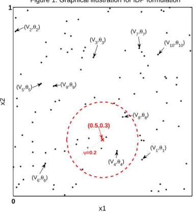
Figure 1. Graphical illustration for lDP formulation
x1
x2
(0.5,0.3)
(V1,θ1) (V2,θ2)
(V3,θ3)
(V4,θ4) (V5,θ5)
(V6,θ6)
(V7,θ7)
(V8,θ8) (V9,θ9)
(V10,θ10)
ψ=0.2
FIGURE 3.1: Black asterisks are the first 100 random locations generated onX0 = [0,1]2 from
H=Uniform([0,1]2). Red dashed circle indicates the neighborhood of the red crossed predictor pointx= (0.5,0.3)0 determined by Euclidian distance d(·) andψ = 0.2. (Vh, θh) forh= 1, . . . ,10
are the the first 10 random pairs of weight and atom assigned to the first 10 random locations Γh for h= 1, . . . ,10.
Figure 3.1 illustrates the lDP formulation graphically for a case where X = [0,1]2 and
GX ∼ lDP(α, G0, H, ψ) with H=Uniform([0,1]2) leading toX =X0 and ψ = 0.2. For a simple
illustration, we consider Euclidian distance ford(·,·) for bivariate predictors. Random locations
in [0,1]2 are generated from a uniform distribution, with the first 100 locations plotted as ’∗’
in Figure 3.1. The random pair of weight and atom (Vh, θh) is placed at location Γh, with the
first 10 pairs labeled in Figure 3.1. For a predictor value x= (0.5,0.3)0, the red dashed circle indicates the neighborhood ofx,ηψ
x. Then,Gx atx= (0.5,0.3)0 is constructed using the weights and atoms within the dashed circle in the order of the index to formulate the stick-breaking representation. For all other x∈ X,Gx are formed following the same steps.
From Figure 3.1, it is apparent that the dependence between Gx and Gx0 increases as the distance between x and x0 decreases. For closer xand x0, their neighborhoods overlap more so that similar components are used for constructing Gx and Gx0, while if x and x0 are far apart, there will be at most a small area of intersection so that few to none of the random components are shared. In the non-overlapping case, Gx and G0x are assigned independent DP priors, as is clear from Theorem 1 and the subsequent development.
Theorem 1. If GX ∼lDP(α, G0, H, ψ), for anyx∈ X, Gx∼DP(αG0).
The marginal DP property shown in Theorem 1 is appealing in allowing one to rely directly on the rich literature on properties of the DP to obtain insight into the prior for the random probability measure at any particular predictor value. However, unlike the DP, the lDP allows the probability measure to vary with predictors, while borrowing information across local regions of the predictor space. This is accomplished through incorporating shared random components. Due to the sharing and to the almost sure discreteness property of eachGx, the lDP will induce local clustering of subjects according to their predictor values. Theorem 2 illustrates this local clustering property more clearly.
Theorem 2. Suppose GX ∼ lDP(α, G0, H, ψ) and φi|Gxi ind
∼ Gxi, for i = 1, . . . , n, with xi
denoting the predictor value for subject i. Then,
κxi,xj = Pr(φi =φj|xi,xj, α, ψ) =
2Pxi,xj
(1 +Pxi,xj)α+ 2
The clustering probability κxi,xj increases from 0 when η ψ
xi T
ηψ
xj = ∅ to 1/(α+ 1) when
xi =xj which is the case of Pxi,xj = 1. This implies that, for fixed α, the clustering probability
under GX ∼ lDP(α, G0, H, ψ) is bounded above by the clustering probability under the global
DP, which takes Gx ≡ G∼ DP(αG0), leading to Pr(φi =φj|α) = 1/(α+ 1). Also, note that
small values of the precision parameter α will induce Vh values that are close to one. This in
turn causes a small number of atoms in each neighborhood to dominate, inducing few local clusters. However, when ψ is small and hence neighborhood sizes are small, there will still be many clusters across X.
It is interesting to consider relationships between the lDP and other priors proposed in the literature in limiting special cases. First, note that the lDP converges to the DP as ψ → ∞, so that all the neighborhoods around each of the predictor values encompass the entire
predictor space. Also, the lDP(α, G0, H, ψ) corresponds to a limiting case of the kernel
stick-breaking process (KSBP) (Dunson and Park, 2008), in which the kernel is defined asK(x,Γ) = 1 d(x,Γ)< ψ and the DP placed at each location have precision parameters→0.
3.3.2
Moments and Correlation
From Theorem 1 and properties of the DP,GX ∼lDP(α, G0, H, ψ) implies, for any x∈ X,
E{Gx(B)}=G0(B) and V ar{Gx(B)}=
G0(B)(1−G0(B))
1 +α , ∀B ∈ B (3.8)
Next, let us consider the correlation between Gx1 and Gx2, for any x1,x2 ∈ X. First, we
show the correlation conditionally on the locations Γ but marginalizing out the weights V and atomsΘ. As discussed in section 3.1, if Γis given, the lDP can be regarded as a special case of the πDDP. Hence, following Theorem 1 in Griffin and Steel (2006), for any x1,x2 ∈ X,
ρx1,x2(Γ) = Corr{Gx1(B), Gx2(B)|Γ}
= 2
α+ 2
X
h∈Lx1∩Lx2
α α+ 2
#Sh
α α+ 1
#Sh0
, ∀B ∈ B, (3.9)
where #S is the cardinality of the set S , Sh = A1h ∩ A2h, Sh0 = A1h ∪ A2h− Sh, and Akh =
{πj(xk) :j < l, πl(xk) =h}for h∈ Lx1 ∩ Lx2. In other words, #Sh is the number of indices on
the locationsΓthat are below h and are shared in the neighborhoods ofx1 andx2, while #Sh0 is
the number of indices that are below h and belong to the neighborhoods of eitherx1 or x2 but
not both. For a givenh, reducing #Sh by one induces adding two elements toSh0, thus reducing
the correlation, as expected. From expression (3.9), it is clear that the neighborhoods around x1 and x2 are increasingly overlapping and the correlation between Gx1 and Gx2 increases as
x1 →x2. Expression (3.9) is particularly useful in being free of dependence onB.
Marginalizing the correlation in (3.9) over the prior for the random locationsΓ is equivalent to marginalizing out the #Sh and #Sh0 for h ∈ Lx1 ∩ Lx2. In considering the correlation
between Gx1 and Gx2, we can ignore the Γh for h ∈ {1, . . . ,∞} \ Lx1 ∪ Lx2 and focus on the
Γh only for h∈ Lx1 ∪ Lx2. Let γj be the jth ordered component of Lx1 ∪ Lx2. For example, if
Lx1 ∪ Lx2 ={1,3,5,6,7,8, . . .}, γ1 = 1, γ2 = 3, γ3 = 5, γ4 = 6,· · ·. LetZγj = 1(γj ∈ Lx1 ∩ Lx2)
be an indicator for whether Γγj are shared by the neighborhoods of x1 andx2 or not. Then, the
formula in (3.9) can be reexpressed with respect toZγj as follows:
ρx1,x2(Γ) = Corr{Gx1(B), Gx2(B)|Γ}
= 2
α+ 2 ∞
X
j=1
Zγj
α α+ 2
Pjk−=11Zγk
α α+ 1
j−1−Pj−1
k=1Zγk
(3.10)
Note that it is straightforward to show that Zγj iid
∼ Bernoulli(Px1,x2), for j = 1, . . . ,∞,
with Px1,x2 =
H(ηψx1
T
ηxψ2)
H(ηψx1
S
ηxψ2)
the conditional probability of Γh falling within the intersection region
ηxψ1 ∩ ηxψ2 given Γh ∈ ηxψ1 ∪ η
ψ
x2. Finally, marginalizing out {Zγj}
∞
j=1 results in the following
Theorem.
Theorem 3. If GX ∼lDP(α, G0, H, ψ), for anyx1,x2 ∈ X,
1 if x1 = x2 which implies the neighborhoods around x1,x2 are identical and Px1,x2=1. Also,
the correlation is 0 when the neighborhoods are non-overlapping with Px1,x2=0. In addition,
Px1,x2 ≤ ρx1,x2 ≤ 1 and ρx1,x2 increases as α increases for fixed Px1,x2. When α → 0, the
correlation converges toPx1,x2. Meanwhile, when α→ ∞, the correlation converges to
2Px1,x2
1+Px1,x2.
Note thatPx1,x2 depends onH,ψ, and the locationsx1 andx2 given a choice ofd(·,·). When
X0 for H is chosen to satisfy Condition 2, some appealing properties result.
Condition 2. For allx∈ X with X being p-dimensional,{x∗;d(x∗,x)< ψ,x∗ ∈ <p} ⊂ X0. From condition 2, one can deduce thatX0 contains all the points in<p within the distance of
ψ fromxfor anyx∈ X. Under condition 2, withH chosen to be a uniform probability measure on a bounded spaceX0,P
x1,x2 depends only onψ andd(x1,x2) which is the distance betweenx1
andx2, but not on the exact locations ofx1 and x2 inX. Hence, upon examination of Theorem
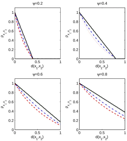
3, it is apparent that condition 2 implies an isotropic correlation structure, which is an appealing default in the absence of prior knowledge of changes in the correlation structure according to the locations inX. Figure 3.2 shows how the correlationρx1,x2 changes as a function ofd(x1,x2)
in the case where x ∈ X = [0,1] and H is Uniform([−ψ,1 +ψ]) so that X0 = [−ψ,1 +ψ] and condition 2 holds for differentψ with d(·,·) corresponding to the Euclidian distance. Theρx1,x2
decays from 1 to 0 as d(x1,x2) increases and the decay is faster for smaller ψ. As ψ → ∞, the
decay line gets closer to a horizontal line at ρx1,x2 = 1, which is the case of lDP=DP. Also, for
a given ψ and d(x1,x2), the ρx1,x2 is higher as α → ∞. Although the choice of d(·,·) being
Euclidian makes the curves in Figure 3.2 close to linear, the curvature can easily be changed by choosing a different distance measured(·,·).
3.3.3
Truncation Approximation
Finite approximations to infinite stick-breaking priors form the basis for commonly-used computational algorithms (Ishwaran and James, 2001). In this subsection, we discuss a finite dimensional approximation to the lDP.
Since the lDP has the marginal DP property, let us recall the finite dimensional DP. Ishwaran
0 0.5 1 0
0.2 0.4 0.6 0.8 1
d(x1,x2)
ρ x,x 1
2
ψ=0.2
0 0.5 1
0 0.2 0.4 0.6 0.8 1
d(x1,x2)
ρ x,x 1
2
ψ=0.4
0 0.5 1
0 0.2 0.4 0.6 0.8 1
d(x1,x2)
ρ x,x 1
2
ψ=0.6
0 0.5 1
0 0.2 0.4 0.6 0.8 1
d(x1,x2)
ρ x,x 1
2
ψ=0.8
FIGURE 3.2: Change in correlation ρx1,x2 over the change in distance d(x1,x2) for different α
and ψ: α = 0.0001 (red dashed), α = 1 (blue dot-dashed), α = 10 (green dotted), α = 10000 (black solid).
and James (2001) defines an N-truncation of the DP (DPN) by discarding theN+1, N+2, . . . ,∞ terms and replacing pN with 1−PN
−1
2,
||µN −µ∞|| ≤4
1−E
N−1 X
h=1
ph n
≈4n×exp{−(N −1)/α}, (3.11)
where || · || is tv norm, µN and µ∞ are the marginal probability measures for the data from the DPMN and DPM models, and n is the sample size. Note that the sample size has a modest
effect on the bound for a reasonably large value of N and the bound decreases exponentially with N increasing, implying that even for a fairly large sample size, the DPMN approximates
the DP well with moderate N.
Following a similar route, let us define an N-truncation of the lDP (lDPN) as follows:
Definition 3. For a finite N, let ΓN = {Γ
h, h = 1, . . . , N}, VN = {Vh, h = 1, . . . , N},
and ΘN = {θ
h, h = 1, . . . , N} be the sets of global random locations, weights, and atoms,
respectively. Distributional assumptions for Γh, Vh, and θh are the same as in (3.5) and the
corresponding local sets are defined as in (3.6). Then, GX ∼lDPN(α, G0, H, ψ) if
Gx =
N(x)−1
X
l=1
pl(x)δθπl(x)+
1−
N(x)−1
X
l=1
pl(x)
δθπN
(x)(x)
with pl(x) = Vπl(x) Y
j<l
(1−Vπj(x)) for l= 1, . . . , N(x)−1
TheGxin Definition 3 has a similar form to G=
PN
h=1phδθh obtained from theDP
N except
that N in G is replaced by N(x) in Gx and N in DPN is fixed while N(x) in lDPN is random. Focusing on a particular predictor value x, it is easy to show that N(x) ∼ Binomial(N,Px), where N is the total number of global locations in lDPN and Px = H(ηxψ) is the probability that a location belongs to the neighborhood around x, ηxψ. Then, marginalizing out N(x) in the bound on the tv distance between the marginal densities of an observation obtained at a particular predictor valuexfrom the lDPM and lDPMN models results in Theorem 4.
Theorem 4. Define a model (3.2) with GX ∼ lDP(α, G0, H, ψ) as local Dirichlet process
mixture (lDPM) model. lDPMN corresponds to (3.2) with G
X ∼ lDPN(α, G0, H, ψ). Suppose
an observation is obtained from lDPMN and lDPM models at x. Then,
||µN(x)−µ∞(x)|| ≤ 4
α+ 1
α
1−
1
α+ 1
Px
N
,
whereµN(x) andµ∞(x) are the marginal probability measures for the observation. Notice that the bound decreases exponentially with N increasing, suggesting that we can obtain a good approximation to the lDP using a moderate N, as long asα is small and the neighborhood size is not too small. In particular, we require a large N for a given level of accuracy asψ →0, since
Px decreases as the size of ηxψ decreases.
3.4
Posterior Computation
We develop an MCMC algorithm based on the blocked Gibbs sampler (Ishwaran and James, 2001) for an lDPMN model. For simplicity in exposition, we describe a Gibbs sampling algorithm for a particular hierarchical model, though the approach can be easily adapted for computation in a broad variety of other settings. We let
f(yi|xi, τ) = Z
f(yi|xi,βi, τ)dGxi(βi) fori= 1, . . . , n
GX ∼ lDPN(α, G0, H, ψ), (3.12)
where f(yi|xi,βi, τ) = N(yi;xi
0
βi, τ−1) with βi = (βi1, . . . , βip)0. For simplicity, we consider
a univariate predictor case where p = 2 and x0i = (1, xi) with d(·,·) Euclidian distance but
the generalization to multiple predictors or to using different distance metric is straightforward.
G0 is assumed to be Np(µβ,Σβ), H is assumed to be Uniform(aΓ, bΓ) and additional conjugate
priors are assigned forτ,α,µβ and Σβ.
the random variables is recast as follows.
(yi|xi,β∗, τ,K) ∼ N(xi
0
β∗Ki, τ−1), i= 1, . . . , n
(Ki|V,Γ) ∼ N(xi)
X
l=1
pl(xi)δπl(xi)(·), i= 1, . . . , n
(Vh|α) ∼ Beta(1, α), h= 1, . . . , N
(Γh) ∼ Uniform(aΓ, bΓ), h= 1, . . . , N
(β∗h|µβ,Σβ) ∼ Np(µβ,Σβ), h= 1, . . . , N
µβ ∼ Np(µ0,Σµ)
Σ−β1 ∼ Wishart({ν0Σ0}−1, ν0)
τ ∼ Gamma(ν1, ν2)
α ∼ Gamma(η1, η2), (3.13)
where β∗ = {β∗h, h = 1, . . . , N}, K = {Ki, i = 1. . . , n}, V = {Vh, h = 1, . . . , N}, and Γ =
{Γh, h= 1, . . . , N}. The full conditionals for each of the random components are based on the
following joint distribution.
(y,K,V,Γ,β∗,µβ,Σβ, τ, α)
∝(y|β∗, τ,K)(K|V,Γ)(V|α)(Γ)(β∗|µβ,Σβ)(µβ)(Σβ)(τ)(α) (3.14)
Then, the Gibbs sampler proceeds by sampling from the following conditional posterior distri-butions:
(a) Conditional forKi, i= 1, . . . , n
(Ki|y,V,Γ,β∗, τ) ∼ N(xi)
X
l=1
p0l(xi)δπl(xi)(Ki)
p0l(xi) =
N(yi;x
0
iβ
∗
πl(xi), τ
−1)p
l(xi) PN(xi)
l=1 N(yi;x
0
iβ
∗
πl(xi), τ
−1)p
l(xi)
pl(xi) = Vπl(xi) Y
j<l
(1−Vπj(xi)) for l < N(xi)
pl(xi) = Y
j<l
(1−Vπj(xi)) for l=N(xi)
(b) Conditional forVh, h= 1, . . . , N
(Vh|K,Γ, α) ∼ Beta(1 + n X
i=1
1(Ki =h and Ki 6=πN(xi)(xi)), α+ n X
i=1
1(Ki > h))
(c) Conditional for Γh, h= 1, . . . , N
(Γh|K,V)∼Uniform(max[ max i;Ki=h
(xi−ψ), aΓ],min[ min
i;Ki=h
(xi+ψ), aΓ])
(d) Conditional forβ∗h, h= 1, . . . , N
(β∗h|y,K,µβ,Σβ, τ) ∼ Np( ˆµβh,Σˆβh)
ˆ
µβh = Σˆβh[Σβ−1µβ+τXihyih]
ˆ
Σβh = [Σβ−1+τXihX0ih]
−1,
whereyih isnh×1 response vector and Xih0 isnh×pdesign matrix for the subjects withKi =h