INTERACTIVE TRACKING, PREDICTION, AND BEHAVIOR LEARNING OF PEDESTRIANS IN DENSE CROWDS
Aniket Bera
A dissertation submitted to the faculty of the University of North Carolina at Chapel Hill in partial fulfillment of the requirements for the degree of Doctor of Philosophy in the Department of
Computer Science.
Chapel Hill 2017
©2017 Aniket Bera
ABSTRACT
Aniket Bera: Interactive Tracking, Prediction, and Behavior Learning of Pedestrians in Dense Crowds. (Under the direction of Dinesh Manocha)
The ability to automatically recognize human motions and behaviors is a key skill for autonomous machines to exhibit to interact intelligently with a human-inhabited environment. The capabilities autonomous machines should have include computing the motion trajectory of each pedestrian in a crowd, predicting his or her position in the near future, and analyzing the personality characteristics of the pedestrian. Such techniques are frequently used for collision-free robot navigation, data-driven crowd simulation, and crowd surveillance applications. However, prior methods for these problems have been restricted to low-density or sparse crowds where the pedestrian movement is modeled using simple motion models.
In this thesis, we present several interactive algorithms to extract pedestrian trajectories from videos in dense crowds. Our approach combines different pedestrian motion models with particle tracking and mixture models and can obtain an average of20%improvement in accuracy in medium-density crowds over prior work. We compute the pedestrian dynamics from these trajectories using Bayesian learning techniques and combine them with global methods for long-term pedestrian prediction in densely crowded settings. Finally, we combine these techniques with Personality Trait Theory to automatically classify the dynamic behavior or the personality of a pedestrian based on his or her movements in a crowded scene. The resulting algorithms are robust and can handle sparse and noisy motion trajectories. We demonstrate the benefits of our long-term prediction and behavior classification methods in dense crowds and highlight the benefits over prior techniques.
TABLE OF CONTENTS
LIST OF TABLES . . . viii
LIST OF FIGURES . . . x
LIST OF ABBREVIATIONS . . . xvii
1 Introduction . . . 1
1.0.1 Pedestrian Movements and Behaviors . . . 2
1.0.2 Motion Models . . . 3
1.0.3 Pedestrian Tracking with Motion Models . . . 4
1.0.4 Pedestrian Prediction . . . 5
1.0.5 Learning Pedestrian Behaviors . . . 5
1.0.6 Crowd Density . . . 6
1.1 Thesis Statement . . . 8
1.2 Main Results . . . 8
1.2.1 Realtime Adaptive Pedestrian Tracking for Crowded scenes . . . 9
1.2.2 Realtime Pedestrian Path Prediction . . . 10
1.2.3 Behavior Learning . . . 12
1.2.4 Applications . . . 13
2 Real-time Pedestrian Tracking . . . 14
2.1 Introduction. . . 14
2.2 Related Work . . . 17
2.3 Microscopic Mixture Motion Model. . . 19
2.3.2 Particle Filter for Tracking . . . 21
2.3.3 Parameterized Motion Model . . . 22
2.3.4 Motion Models . . . 22
2.3.4.1 Reciprocal Velocity Obstacles . . . 23
2.3.4.2 The Boids Model . . . 23
2.3.4.3 Social Forces Model . . . 24
2.3.5 Microscopic Mixture of Motion Models . . . 24
2.3.6 Adaptive Particle Selection . . . 29
2.3.6.1 Computing Pedestrian Clusters . . . 30
2.3.6.2 Macroscopic/Continuum Representation . . . 31
2.3.7 Evaluation Metrics . . . 33
2.4 Model Analysis . . . 34
2.4.1 Tracking Evaluation . . . 38
2.4.2 Tracking Results . . . 38
2.4.3 Implementation Details . . . 40
2.5 Limitations, Conclusions, and Future Work . . . 42
3 Realtime Pedestrian Path Prediction using Global and Local Movement Patterns . . . 43
3.1 Introduction. . . 43
3.2 Related Work . . . 46
3.2.1 Path Prediction . . . 46
3.3 Real-time Pedestrian Path Prediction . . . 47
3.3.1 Pedestrian State Estimation . . . 47
3.3.2 Global Movement Pattern . . . 49
3.3.3 Local Movement Pattern . . . 50
3.3.4 Prediction Output . . . 51
3.4 Analysis . . . 52
3.4.2 Long-term Prediction Accuracy . . . 54
3.4.3 Varying the Pedestrian Density . . . 55
3.4.4 Varying the Sampling Rate . . . 55
3.4.5 Comparison with Prior Methods . . . 56
3.4.6 Implementation Details . . . 57
3.5 Limitations, Conclusions, and Future Work . . . 57
4 Learning Pedestrian Behaviors . . . 59
4.1 Introduction. . . 59
4.2 Related Work . . . 62
4.2.1 Video-Based Crowd Analysis . . . 62
4.2.2 Pedestrian Behavior Modeling . . . 63
4.3 Pedestrian Behavior Computation . . . 63
4.3.1 Personality Trait Classification . . . 64
4.3.2 Global Characteristics . . . 65
4.3.3 Simulated Crowd Behavior Analysis & Prediction . . . 68
4.4 Performance and User Evaluation . . . 68
4.4.1 Performance Evaluation . . . 68
4.4.2 User Evaluation . . . 69
4.5 Conclusions, Limitations, and Future Work . . . 70
5 Applications . . . 73
5.1 Data-driven Crowd Simulation . . . 73
5.1.0.1 Crowd Replication . . . 74
5.1.0.2 Mixing Crowd Streams . . . 76
5.1.1 Crowd Content Generation . . . 76
5.1.1.1 Augmented Crowds . . . 76
5.2 SocioSense: Socially-Aware Robot Navigation . . . 82
5.2.2 Personality Traits and Psychological Cues . . . 84
5.2.3 Pedestrian Path Prediction . . . 85
5.2.4 Proxemic Distances (Social Cues) . . . 86
5.2.5 Socially-Aware Robot Navigation . . . 87
5.2.6 Performance and Analysis . . . 88
5.2.7 Prediction Accuracy . . . 89
5.2.8 Socially-aware Navigation . . . 90
5.3 Anomaly Detection . . . 92
5.3.1 Related Work . . . 93
5.3.2 Approach . . . 93
5.3.2.1 Motion segmentation . . . 94
5.3.2.2 Anomaly detection . . . 95
5.3.3 Quantitative Results . . . 96
6 Conclusion and Future Work . . . 100
LIST OF TABLES
1.1 We define our classification for different pedestrian densities . . . 7
2.1 Initial motion model parameters for optimization. . . 39
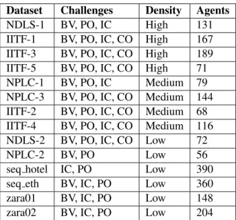
2.2 Crowd Scenes used as Benchmarks. We highlight many attributes of crowd videos including density and the number of pedestrians tracked. We use the following abbreviations about the underlying scene: Background Variations(BV), Partial
Occlusion(PO), Complete Occlusion(CO), and Illumination Changes(IC). . . 40
2.3 We compare the MOTA and MOTP values across the density groups and the
different motion models. . . 40
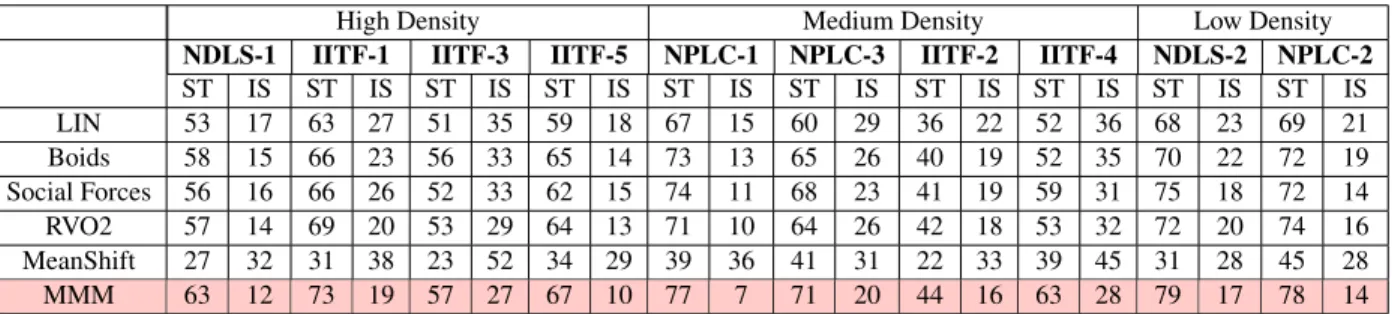
2.4 We compare the percentage of successful tracks (ST) and ID switches (IS) of our Mixture Motion Model algorithm (MMM) with homogeneous motion models - LIN, Boids, Social Force, LTA, RVO2, and a baseline mean-shift tracker. Our method provides higher accuracy compared to homogeneous motion models and lesser ID switches. The benefits of our approach are higher, as the crowd density increases.
These datasets are publicly available at http://gamma.cs.unc.edu/RCrowdT/. . . 41
3.1 Crowd Scene Benchmarks: We highlight many attributes of these crowd videos, including density and the number of tracked pedestrians. We use the following abbreviations about some characteristics of the underlying scene: Background Variations (BV), Partial Occlusion (PO), Complete Occlusion (CO) and Illumina-tion Changes (IC). We highlight the results for short-term predicIllumina-tion (1 sec) and long term prediction (5 sec). We notice that our GLMP algorithm results in higher accuracy for long-term prediction and dense scenarios. More details are given in
Section IV(B). . . 53
4.1 Performance of PTC (Personality Trait computation) and GMD (Global Movement Dynamics) algorithms on different crowd videos. We highlight the number of pedestrians used for personality classification, the number of video frames used for extracted trajectories, and the running time (in seconds). In the PBS Presidential Inauguration video, we chose around130representative pedestrians in the video
for analysis and prediction. . . 69
4.2 Correspondence between six personality traits and the PEN model (Pervin, 2003). . . 70
5.1 Extraversion vs Personal/Social Distances:The personal distance indicates the minimum distance before the pedestrian feels uncomfortable with the robot. All
5.2 Accuracy Benchmarks: We compare our path prediction algorithm with state of the art real-time algorithms, on crowd video datasets with varying densities and numbers of tracked pedestrians, and time windows of 1 sec and 5 sec. Our approach, SocioSense, consistently outperforms the other methods, even for chal-lenging datasets like Marathon. Abbreviations used for scene characteristics: BV: Background Variations, PO: Partial Occlusion, CO: Complete Occlusion, IC:
Illumination Changes. . . 89
5.3 Navigation Performance: A robot using ourSocioSense navigation algorithm can reach its goal position, while ensuring that the personal/social space of any pedestrian is not intruded with<30% overhead. We evaluated this performance in a simulated environment, though the pedestrian trajectories were extracted from
the original video. . . 91
5.4 Performance of trajectory level behavior learning on a single core for different benchmarks: We highlight the number of frames of extracted trajectories, the time spent in learning pedestrian behaviors (BLT - Behavior Learning Time (in sec)). Our learning and trajectory computation algorithms demonstrate interactive
performance on these complex crowd scene analysis scenarios. . . 98
5.5 Comparison of Anomaly Detection techniques. All the reference methods have been explained in detail in (Li et al., 2015). Our method has comparable results
with the state of the art offline methods in anomaly detection. . . 99
LIST OF FIGURES
1.1 The modeling of pedestrian movements has received considerable attention in multiple fields, including computer-aided design, urban planning, robotics, and evacuation planning. In many of these applications, the goal is to capture the tra-jectories and behaviors of the pedestrians. This image shows a subset of the many applications that model pedestrian movements (e.g., pedestrian movement predic-tion, personality recognipredic-tion, data-driven crowd simulapredic-tion, large-scale tracking,
etc.). . . 1
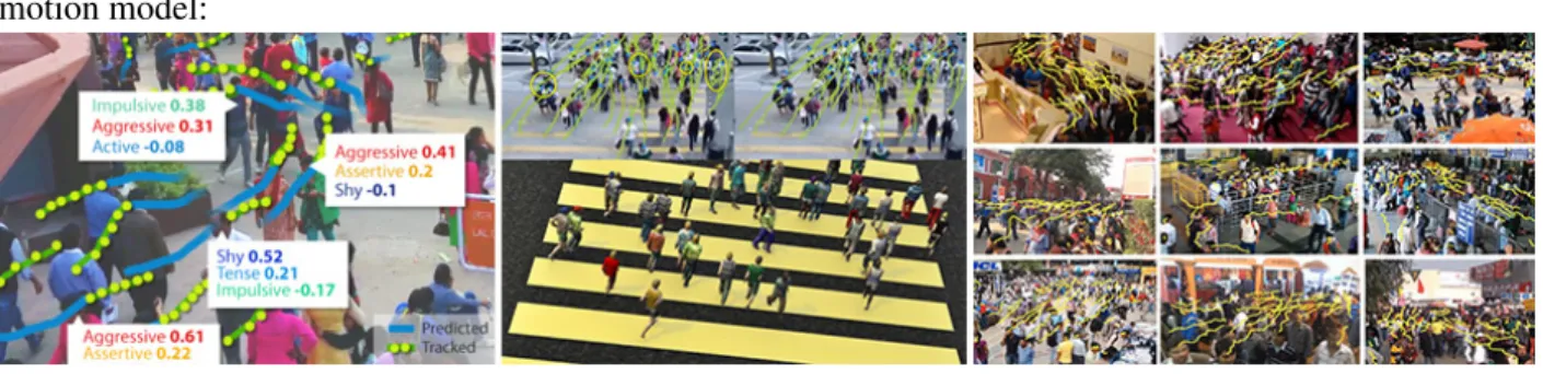
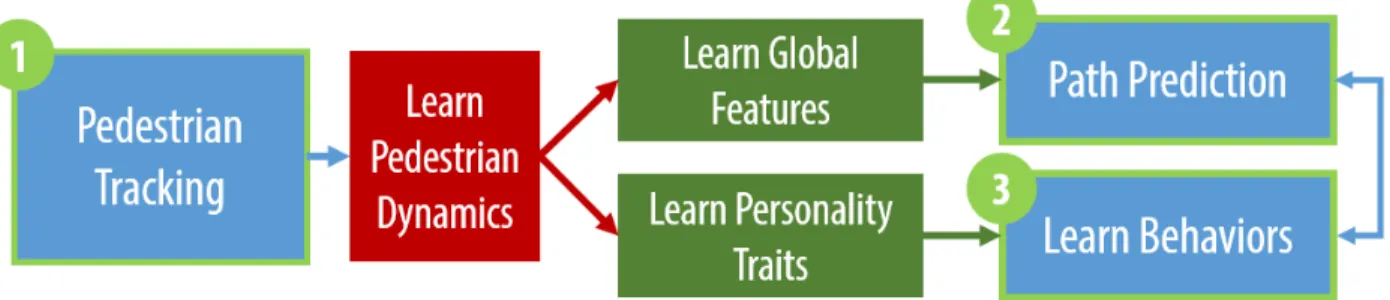
1.2 Overview: We highlight the different aspects of movements (tracked trajectories marked with yellow in (1), predicted trajectories as blue dots in (2) and
personali-ties/behaviors in (3)) of pedestrians in the same scene. . . 3
1.3 We show crowds at different densities (pedestrian marked with ared dot). We define low density as crowds with 0–1 pedestrians per squared-meter, medium density as 1–3 pedestrians per squared-meter and more than 3 pedestrians per
squared-meter as high density. . . 7
1.4 Overview:In this thesis, we present several interactive algorithms to extract pedes-trian trajectories from videos in dense crowds. Our approach combines different pedestrian motion models with particle tracking and a mixture of motion models. We compute the pedestrian dynamics (a collection of different behavior and move-ment patterns, (Kim & Bera et al. 2014)) from these trajectories using Bayesian learning techniques and combine with global methods for long-term pedestrian prediction in dense crowds. Finally, we combine these techniques with Personality Trait Theory from Psychology to automatically classify the dynamic behavior or personality of a pedestrian based on his or her movements in a crowded scene. The resulting methods are robust and can handle sparse and noisy trajectories. We demonstrate the benefits of our long-term prediction and behavior classification
methods in dense crowds and highlight the benefits over prior techniques. . . 8
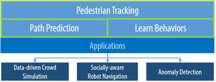
1.5 Application:We demonstrate the performance of our novel algorithms on three different applications. The first application is an interactive data-driven crowd simulation that includes crowd replication, crowd merging, and a combination of pedestrian behaviors from different videos. Secondly, we combine the prediction scheme with proxemic characteristics from psychology and use the result to per-form socially-aware navigation. Finally, we present novel techniques for anomaly detection in low to medium density crowd videos using trajectory-level behavior
learning. . . 9
1.6 We highlight different motion models (Boids, Social-Forces, or reciprocal velocity obstacles) used for the same pedestrian (marked in red) over different frames/time. We believe that it is not possible to model the trajectory of all pedestrians based on a single, homogeneous motion. Instead, we adaptively choose the best-fit model for every pedestrian in the scene, which can vary based on the environment or the
1.7 Prediction Overview: We highlight various components of our real pedestrian path prediction algorithm. Our approach computes both local and global movement patterns using Bayesian inference from 2D trajectory data and combines them to
improve prediction accuracy . . . 11
1.8 Behavior Learning:Our approach can automatically classify the behavior of each pedestrian in real-time. This behavior information is used to dynamically compute the motion parameters and improve the performance of our long term prediction algorithm (shown in dark blue). Our results are very close to ground truth (shown in red) and offer up to 24% improvement over prior real-time prediction algorithms,
whose predicted trajectories are shown in different colors. . . 12
2.1 Improved Realtime TrackingThe results of our approach on some challenging datasets. We highlight the performance of our algorithm for realtime tracking of pedestrians in indoor and outdoor scenes (shown above) with many tens of pedestrians. In such challenging scenarios, our algorithm can track up to 79% of pedestrians in a frame at 26 fps (on average). We observe up to 20% improvement
in the accuracy over prior interactive methods. . . 15
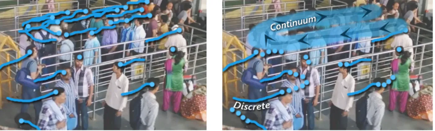
2.2 The left image highlights the tracked trajectories based on discrete motion models. The image on the right demonstrates the use of a hybrid motion model, using the continuum method for a cluster of pedestrians as well as discrete motion models for individuals. These clusters are computed in realtime based on frame coherence and pedestrian flow. The hybrid motion model can improve the tracking accuracy
in these dense scenarios by 20% over prior methods. . . 16
2.3 Our microscopic mixture motion model can accurately compute the trajectories in real time. We highlight different motion models (Boids, Social-Forces, or reciprocal velocity obstacles) used for the same pedestrian (marked in red) over different frames. We believe that it is not possible to model the trajectory of all pedestrians based on a single, uniform model. Instead, we adaptively choose the best-fit model for every pedestrian in the scene that can be adapted to the
environment or the crowd conditions . . . 17
2.4 Overview of our real time tracking algorithm. The symbols used in this figure are explained in Section 2.3.1. We use the trajectory computed over prior k frames, expressed as a succession of states, to compute the new motion model; we use our
microscopic mixture motion model to compute the next states using a particle filter. . . 20
2.5 Our parameter optimization algorithm used in Figure 2.4. Based on the error metric, we compute optimal parameters for each motion model. The best motion model (from RVO2, Social Forces, Boids or LIN) is used for trajectory extraction and to
predict the next state. . . 25
2.6 Comparing the score of the different optimization approaches. Each graph is a range of the scores (minimum and maximum) and the black dot is the mean score. We compute the score from the normalized error metric. A lower value indicates
2.7 The three different categories of crowds based on increasing level of inter-pedestrian interaction: 1) Mostly unidirectional flow, 2) evenly distributed flow/crossflow, 3)
high degree of randomness/no strong flows visible . . . 35
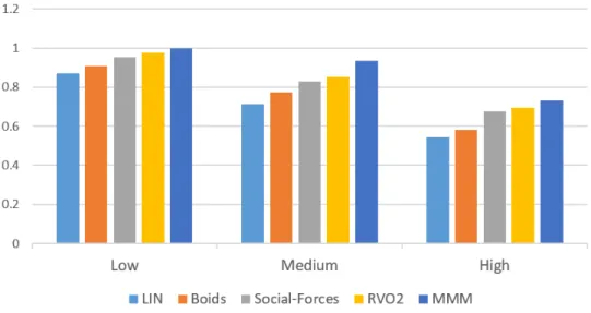
2.8 Benchmarks: Comparative scores (y-axis, lower is better) of the Boids-like, Social-force and RVO2 and LIN models at three different densities. Note: The
fundamental diagram metric was only analyzed for medium and high density videos. . . 37
2.9 We visually analyze the data in Table 2.3 normalized MMM (Low Density) as a baseline. . . 39
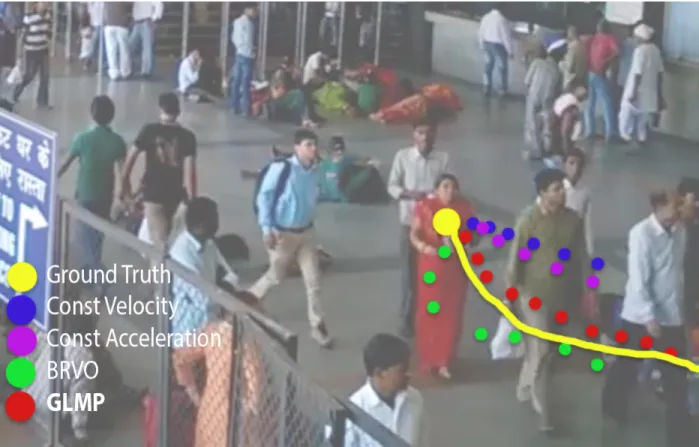
3.1 Improved PredictionWe demonstrate the improved accuracy of our pedestrian path prediction algorithm (GLMP) over prior real-time prediction algorithms (BRVO, Const Vel, Const Accel) and compare them with the ground truth. We
observe upto 18% improvement in accuracy. . . 44
3.2 We highlight various components of our real pedestrian path prediction algorithm. Our approach computes both local and global movement patterns using Bayesian
inference from 2D trajectory data and combines them to improve prediction accuracy. . . 45
3.3 Prediction Outputs We test our approach on a variety of crowd datasets with varying density. Our approach had a benefit of upto 18% better prediction at a 5 second time horizon for some high-density datasets. Yellow lines represent past
tracked trajectories whereas the red dots represent predicted motion. . . 47
3.4 Global vs Local Movement PatternsThe blue trajectories indicate prior tracked data. The red dots indicate local predicted patterns retrieved from learning macro and microscopic simulation models, The shaded (green-blue) path represent the
global movement patterns learned from the path data in that cluster . . . 48
3.5 Improved PredictionWe demonstrate the improved accuracy of our pedestrian path prediction algorithm (GLMP) over prior real-time prediction algorithms
(BRVO, Const Vel, Const Accel). . . 52
3.6 Prediction Accuracy vs. Sensor Error (higher is better)We increase the sensor noise (Gaussian) from left to right and highlight the prediction accuracy across various distance thresholds. The X-axis represents the percentage of correctly predicted paths within varying accuracy thresholds. In this GLMP results in more accurate predictions, as compared to BRVO, Constant Velocity, Constant
Acceleration. As the sensor noise increases (c), we observe more significant benefit. . . 54
3.7 Errors for varying Pedestrian Densities (lower is better). In low-density sce-narios, local movement patterns (e.g BRVO) are able to predict the positions well, but are more accurate than const. velocity and const. acceleration. We observe
improved accuracy with GLMP, as the pedestrian density increases. . . 55
3.8 Error vs Sampling IntervalAs the sampling interval increases, the error from Constant Velocity, Constant Acceleration and BRVO grows much larger than that
3.9 Error Reduction Comparison We compare the improvements of our method, LTA, ATTR and BRVO over LIN (linear velocity) model. Our method (GLMP) outperforms LTA, ATTR with 24-47% error reduction rate in all three different
scenarios. . . 57
4.1 Crowd Behavior Learning/Prediction: Our approach can automatically classify the behavior of each pedestrian in a large crowd. We highlight its application for the 2017 Presidential Inauguration crowd video at the National Mall at Washington, DC (courtesy PBS): (1) original aerial video footage of the dense crowd; (2) a synthetic rendering of pedestrians in the red square based on their personality classification: aggressive (orange), shy (black), active (blue), tense (purple), etc; (3) a predicted simulation of 1M pedestrians in the space with a similar distribution
of personality traits. . . 60
4.2 Our method takes a streaming crowd video as an input. We compute the state of pedestrians in the crowd, as explained in Section 3. Based on the state information, we learn local and global behavior properties, which are combined for behavior
classification and prediction. . . 62
4.3 Personality Classification: We identify the personality of each tracked pedestrian based on pedestrian dynamics and the motion model. Each pedestrian is
automati-cally classified using a weighted combination of different personality traits. . . 65
4.4 Participant Responses Using the Six Factor Personality Model: Participants were shown 10 different videos of pedestrians walking among crowds. In each video, a single pedestrian was highlighted and participants were asked to report the most appropriate personality trait for that pedestrian. 31 participants reported the most appropriate personality trait from the given set: Aggressive, Impulsive, Active,
Assertive, Tense, and Shy. . . 71
4.5 Participant Responses Using the PEN Model: We converted the participant re-sponses to the three factor PEN model to reduce the disagreement. Participant responses were converted to three PEN factors (Psychoticism, Extraversion, and
Neuroticism) using Table 4.2. . . 72
4.6 Accuracy of our PTC Algorithm: Our PTC algorithm predicted the most dominant trait for each of the 7 videos. In 76.96% of the cases, participants also chose the most dominant trait as denoted by the dark green color. If we also add the second most dominant trait (denoted by light green), the accuracy increased to 88.48%. This accuracy indicates that our PTC algorithm was able to correctly identify the
5.1 Noisy vs. Smooth trajectories: The red trajectories were tracked using LIN (con-stant velocity) as the motion model and the blue trajectories are results from our baseline tracking algorithm (Chapter 2). We display the improved trajectories extracted by our algorithm in green, which are smoother. Our motion model it-eratively refines pedestrian behavior and produces smooth trajectories. The blue circles highlight the improvement using our method. (For clarity, these trajectories
are just a cropped section of the entire scene.) . . . 74
5.2 Augmented Crowd Video:Our approach can be used to augment a crowd video with additional virtual agents. (a) We use an outdoor crowd scene (Crossing bench-mark (Shao et al., 2014)) as a background. (b) We extract pedestrian trajectories from a different video benchmark (Manko benchmark (Shao et al., 2014)) (c) We add computer-simulated virtual pedestrians following behaviors observed in the Manko video dataset. (d) The resulting trajectories are rendered and overlaid upon the Crossing video dataset. We use chroma keying to insert these new virtual agents into the original video, which includes additional environmental features,
such as moving cars. . . 74
5.3 Replicated Crowds. We improve the quality of the rendered crowd behaviors by adding online smoothing step to the tracker. (a) to (d) shows the replicated crowds rendered directly using the tracking results without any pre-processing,
corresponding to each benchmark video. . . 75
5.4 Mixing Crowd Streams: The agents on the brown (left) and blue (central) floors exhibit varied behaviors, generated from different videos. The final mixed video (green floor) has behaviors combined from both the video streams. Pedestrians marked with brown are from the left video, and those marked blue are from the central video. The overall mixing algorithm uses the two sets of extracted
trajectories and performs local collision avoidance between them. . . 77
5.5 Mixing trajectories from multiple input videos.We can use multiple videos as inputs to a single, more complex scenario. In the left two videos of (a), pedestrians move in an image-space from bottom to top or from top to bottom. In the right two videos of (a), pedestrians move in a uniform direction: right to left in a slightly tilted way in the image-space. There are, therefore, three different main directions of pedestrian movements. (b) Using these trajectories with agent-based simulation methods, we can generate crowds with these three different flows, while still
achieving local collision avoidance between the agents. . . 78
5.6 Comparison of improved tracking (our method, above) to prior methods based on particle filter + LIN (below). We compare the quality of the extracted trajectories on four different real crowd videos. As compared to prior methods, our approach results in smoother trajectories and improved accuracy for each
5.7 Augmented Crowd We use pedestrian tracking results for crowd content gen-eration. In this scenario, we add virtual pedestrians to the scene and generate collision-free trajectories for them at interactive rates. (a) Trajectories of 23 real pedestrians in an open space; (b) adding 50 virtual pedestrians; (c) adding 300
virtual pedestrians; . . . 79
5.8 Augmented Crowd Rendered in a 3D Environment(a) Original Dawei video dataset with tracked trajectories, from which 27 trajectories are extracted; (b) Rendered scene with real and randomly inserted virtual pedestrians with similar trajectory-level behaviors, in which100virtual pedestrians have been added; and
(c) Rendered scene with real and virtual agents using our behavior-learning approach. . . 80
5.9 Improved Navigation usingSocioSense:(a) shows a real-world crowd video and the extracted pedestrian trajectories in blue. The green markers are the predicted positions of each pedestrian computed by our algorithm that are used for collision-free navigation. The red and yellow circles around each pedestrian in (b) and (c) highlight their personal and social spaces respectively, computed using their personality traits. We highlight the benefits of our navigation algorithm that accounts for psychological and social constraints in (c) vs. an algorithm that does not account for those constraints in (b). The red trajectory of the white robot maintains these interpersonal spaces in (c), while the robot navigates close to the
pedestrians in (b) and violates the social norms. . . 83
5.10 Example robot trajectorynavigating through the crowd inHoteldataset. Red/yel-low circles represent current pedestrian positions(personal/social distance), green
circles are the current position of the robot. . . 88
5.11 Our robot navigation algorithm satisfies the proxemic distance constraints, includ-ing personal space (red) and social space (yellow). The trajetory computed by our SocioSense navigation algorithm (green trajectory) does not intrude on the person-al/social space of the pedestrian, whereas a robot that fails to take into account the
social constraints (purple trajectory) may cause discomfort to the pedestrians. . . 90
5.12 Our approach automatically classifies pedestrian behaviors in real-time (e.g. Shy behavior of a pedestrian). This behavior information is used to dynamically com-pute motion parameters and improve the performance of our long-term prediction algorithm (shown in dark blue) and compute proxemic distances. Our results are very close to ground truth (shown in red) and offer up to 21% improvement over prior real-time algorithms, whose predicted trajectories are shown in different colors. This demonstrates the benefits of using the psychological constraints for
prediction and navigation. . . 91
5.13 Motion segmentation of structured and unstructured scenarios:Different col-ors indicate clusters grouped by similarity of behavior or movement features at interactive rates. We use eight discrete colors for visualization of the results in
5.14 Anomaly Detection. We also evaluate other datasets like UCSD. Trajectories of 63 real pedestrians are extracted from a video. One person in the middle walks against the flow of crowd. Our method can capture the anomaly of this pedestrian’s behavior or movement by comparing the behavior features with those of other
LIST OF ABBREVIATIONS
ORCA Optimal Reciprocal Collision Avoidance PDL Pedestrian Dynamics Learning
RVO Reciprocal Velocity Obstacle
MMM Motion Model Mixture
GLMP Realtime Pedestrian Path Prediction usingGlobal andLocalMovementPatterns PTC Personality Trait computation
GMD Global Movement Dynamics GVO Generalized Velocity Obstacles
CHAPTER 1 Introduction
The ability to automatically recognize human movements and activities is key for autonomous machines to interact intelligently with a human-inhabited environment (i.e. humans walking towards their goal and avoiding collisions with other humans and obstacles while interacting with the environment). The possibility of sensing human crowd motion has received considerable attention in the literature. It is a well-studied problem that has applications in many domains. For example, it is considered in computer animation to generate human motion for special effects (Kovar et al., 2002; Badler, 1997a). In virtual environments, it is used to generate movements and interactions for human avatars and virtual agents (Baylor, 2009; Bainbridge, 2007; Badler, 1997b). Surveillance applications include evaluating atypical and suspicious movements that differ from those of the crowd (Wu et al., 2010; Mahadevan et al., 2010). Similarly, behavior modeling discusses this problem as it relates to the analysis of personalities and behaviors based on their interaction in the real world (Cristani et al., 2013; Yi et al., 2015). In other applications, this problem has implications for disaster prevention and planning evacuations, crowd scene analysis (analyzing global characteristics of the crowd), and collision-free navigation of robots or autonomous vehicles in crowded or real-world scenarios. The following are some specific applications that best illustrate the need for a better pedestrian or crowd motion model:
• As robots are increasingly used in households, offices, and public places, they navigate among humans or pedestrians more and more. Because humans are dynamic agents (changing directions, positions, etc.), these scenarios result in many new challenges related to navigation and the awareness of human motion and interactions. Robots must move through crowds of people while preventing collisions with each other and humans. In such scenarios, the robots need to interface with not only the physical environment, but also the social environment, and should interact well with pedestrians.
• One of the key challenges in surveillance is to devise methods that can automatically analyze the behavior and movement patterns in crowd videos to detect anomalous or atypical behaviors (Li et al., 2015). Furthermore, since many of the surveillance systems need realtime planning for security, most of these applications benefit from interactive performance, and do not rely on a priori learning or labeling. However, current methods are typically limited to sparse crowds or are designed for offline or non-realtime applications.
• Crowds have also been studied in computer animation for use in generating special effects. Frequently, designers or animators must go through a tedious process to generate scene-specific behavior rules such as events, trajectories, or interactions. To account for these factors, they have to manually generate scene-specific behaviors or trajectories. This can be time consuming and, further, generating realistic behaviors or simulations using such methods involves considerable tweaking of or variations in simulation parameters. As the number of agents or the complexity of the scenarios increases, it becomes increasingly difficult to model the diversity of behaviors or the interactions between the agents.
1.0.1 Pedestrian Movements and Behaviors
From the problems and applications described above, it is apparent that it is important to design and develop algorithms which not only efficiently capture pedestrian motion and behavior, but do it interactively. This interactivity is especially important for applications such as realtime surveillance, autonomous vehicle planning, and robot planning. For this work, we consider capturing pedestrian motion and behavior as a collection of three interconnected components:
Figure 1.2:Overview: We highlight the different aspects of movements (tracked trajectories marked with yellow in (1), predicted trajectories as blue dots in (2) and personalities/behaviors in (3)) of pedestrians in the same scene.
• Prediction: Determining future pedestrian positions and velocities based on past data. We define short term prediction as future pedestrian positions for 1–2 seconds and long term prediction as future positions for 5 or more seconds.
• Behavior Learning: For this work we restrict ourselves to trajectory-level motion patterns and personality traits based on prior work in psychology and various interactions with environment.
We take these three important problems and classify them as a part of ‘pedestrian sensing’. However, sensing pedestrians in a crowded scene is regarded as a difficult problem due to, for example, intra-pedestrian occlusion (i.e. one pedestrian blocking others) and changes in lighting and pedestrian appearance. Similarly, predicting the trajectory of a pedestrian in a dense environment can also be very challenging. In general, pedestrians have varying behaviors and can change their speed to avoid collisions with the obstacles and other pedestrians in a scene. In crowded scenarios, the interactions between the pedestrians tend to increase significantly, which affects their behavior and movement. While researchers in various fields like psychology and other social sciences have been studying and observing human behavior for decades, modeling realistic crowd behaviors is challenging. Further, there are no widely accepted models capable of capturing a wide variety of behaviors. As a result, the highly dynamic nature of pedestrian movement makes it hard to estimate a pedestrians current or future positions.
1.0.2 Motion Models
body of work in robotics, multi-agent systems, crowd simulation, and computer vision on modeling pedestrian motion in crowded environments. We limit the scope of the motion models discussed in this thesis to those that mainly compute trajectory-level movements or behaviors of each independent individual, which we call theagentorpedestrian, in the crowd. These models can be broadly classified into the following categories: potential-based models, which model virtual agents in a crowd as particles with potentials and forces (Helbing and Molnar, 1995a); boid-like approaches, which create simple rules to steer agents (Reynolds, 1999a); geometric optimization models, which compute collision-free velocities (Van Den Berg et al., 2011a); and field-based methods, which generate fields based on continuum theory (Treuille et al., 2006). Among these approaches, velocity-based motion models (Karamouzas et al., 2009; Karamouzas and Overmars, 2010; van den Berg et al., 2008b; Van Den Berg et al., 2011a; Pettr´e et al., 2009) have been successfully applied to the simulation and analysis of crowd behaviors and to multi-robot coordination (Snape et al., 2011). Velocity-based models have also been shown to have efficient implementations that closely match real human paths (Guy et al., 2010). These models form the basis for modeling the pedestrian motion in our work (i.e. pedestrian tracking, prediction, and behavior learning).
1.0.3 Pedestrian Tracking with Motion Models
are slow and work offline. Additionally, these methods are well-suited for modeling motion in dense crowds with few distinct motion patterns; however, they may not work in heterogeneous crowds.
1.0.4 Pedestrian Prediction
Crowd trajectory prediction has been studied extensively for robot navigation and related areas. (Fulgenzi et al., 2007) use a probabilistic velocity-obstacle approach combined with dynamic occupancy grid. This method assumes constant linear velocity motion of the obstacles. (Du Toit and Burdick, 2010) present a robot planning framework that accounts for each pedestrian’s anticipated future location information to reduce the uncertainty of the predicted belief states. Other techniques use potential-based approaches for robot path planning in dynamic environments (Pradhan et al., 2011). Some methods learn the trajectories from collected data. (Ziebart et al., 2009a) use pedestrian trajectories collected in the environment for prediction using Hidden Markov Models. (Bennewitz et al., 2005) apply Expectation Maximization clustering to learn typical motion patterns from pedestrian trajectories before using Hidden Markov Models to predict future pedestrian motion.(Henry et al., 2010) use reinforced learning from example traces, estimating pedestrian density and flow with a Gaussian process. (Kretzschmar et al., 2014) consider pedestrian trajectories as a mixture probability distribution of a discrete as well as a continuous distribution, and then use Hamiltonian Markov chain Monte Carlo sampling for prediction. (Kuderer et al., 2012) use maximum entropy-based learning to learn pedestrian trajectories and use a hierarchical optimization scheme to predict future trajectories. Many of these methods involve a priori learning and may not work in new or unknown environments. Variations of Bayesian filters for pedestrian path prediction have been studied in (Schneider and Gavrila, 2013; Mogelmose et al., 2015). Most of these methods are not suitable for real-time applications or may not work well for dense crowds. They also tend to fail for trajectories predicted over a longer time (>5seconds).
1.0.5 Learning Pedestrian Behaviors
and detailed behaviors when used with corresponding scenarios such as buying a ticket or waiting in line. Also, Finite State Machines (FSM) are commonly used to encode procedural behaviors or a set of goals based on an agent’s state (Bandini et al., 2006; Paris and Donikian, 2009; Sean Curtis, 2013). There is also recent work on analyzing pedestrian motion patterns on a semantic-level (Wang et al., 2017, 2016).
There is extensive work in computer vision, multimedia, and robotics that analyzes the behaviors and movement patterns in crowd videos, as surveyed in (Li et al., 2015; Borges et al., 2013). The main objectives of these works include human behavior understanding and crowd activity recognition for the detection of abnormal behaviors (Hu et al., 2004). Many of these methods use a large number of training videos to learn the patterns offline (Zen and Ricci, 2011; Solmaz et al., 2012). Other methods utilize motion models to learn crowd behaviors (Pellegrini et al., 2012) or use machine learning algorithms (Zhou et al., 2012b; Cheung et al., 2016). Some techniques focus on classifying the most common behavior patterns in a scene using offline learning. These include activity prototypes using a convex learning algorithm (Zen and Ricci, 2011) and detection of popular behavior patterns like bottlenecks, fountainheads, lanes, arches, and blocking (Solmaz et al., 2012).
Crowd behavior learning using motion or simulation has been used for different applications. Parameter learning has been used to predict pedestrian motion for tracking (Pellegrini et al., 2012). However, these techniques use either manual selection or offline learning techniques to estimate the goal positions. Other researchers have used low-density tracking data to learn agent intentions (Musse et al., 2007) or online Bayesian motion-prediction methods for human-robot interactions, data-driven crowd simulation (Kim et al., 2016), and offline training (Zhong et al., 2015). Different approaches have been used to model pedestrian behavior. (Funge et al., 1999) use cognitive modeling to empower agents to plan and perform high-level tasks (Godoy et al., 2016).
1.0.6 Crowd Density
Density Average pedestrians/m2
Low <1
Medium 1–3
High >3
Table 1.1: We define our classification for different pedestrian densities
As a general rule, the higher the density the more difficult it becomes to track/predict pedestrian motion. In most cases, the appearance model (algorithm for matching a statistical model of object shape and appearance to a new image) isn’t capable of capturing partially-visible pedestrians in a crowd.
Figure 1.4:Overview:In this thesis, we present several interactive algorithms to extract pedestrian trajectories from videos in dense crowds. Our approach combines different pedestrian motion models with particle tracking and a mixture of motion models. We compute the pedestrian dynamics (a collection of different behavior and movement patterns, (Kim & Bera et al. 2014)) from these trajectories using Bayesian learning techniques and combine with global methods for long-term pedestrian prediction in dense crowds. Finally, we combine these techniques with Personality Trait Theory from Psychology to automatically classify the dynamic behavior or personality of a pedestrian based on his or her movements in a crowded scene. The resulting methods are robust and can handle sparse and noisy trajectories. We demonstrate the benefits of our long-term prediction and behavior classification methods in dense crowds and highlight the benefits over prior techniques.
1.1 Thesis Statement
Our thesis statement is as follows:
Higher order motion models and learning techniques can be used to design accurate algorithms for
pedestrian tracking, long term prediction and behavior learning.
In this thesis, we propose interactive algorithms to track, predict and learn pedestrian behaviors. A large part of our research borrows ideas related to understanding and observing human-like behaviors and their interactions from other fields including psychology, physics, and machine learning. As a result, both short-term, local interaction and long-term, high-level behavior models are improved. Our approaches use online methods to learn the trajectory-level behaviors for each agent by combining non-linear motion models and Bayesian inference. Moreover, we highlight applications of our pedestrian tracking, prediction and behavior learning algorithms to many different areas, including computer animation, computer vision, and robotics.
1.2 Main Results
Figure 1.5:Application:We demonstrate the performance of our novel algorithms on three different applica-tions. The first application is an interactive data-driven crowd simulation that includes crowd replication, crowd merging, and a combination of pedestrian behaviors from different videos. Secondly, we combine the prediction scheme with proxemic characteristics from psychology and use the result to perform socially-aware navigation. Finally, we present novel techniques for anomaly detection in low to medium density crowd videos using trajectory-level behavior learning.
1.2.1 Realtime Adaptive Pedestrian Tracking for Crowded scenes
We present new pedestrian tracking algorithms that are based on the use of particle filters to perform realtime pedestrian tracking in moderately crowded scenes. We use the notion of a crowd model as a motion prior. We demonstrate that using a crowd motion model (in this case, specifically using velocity obstacles) can improve pedestrian tracking in dense scenes, compared to using a constant velocity or constant acceleration model. Ours is also a hybrid approach which is computationally optimized and is adaptive to the crowd size, dynamics etc.
Figure 1.6: We highlight different motion models (Boids, Social-Forces, or reciprocal velocity obstacles) used for the same pedestrian (marked in red) over different frames/time. We believe that it is not possible to model the trajectory of all pedestrians based on a single, homogeneous motion. Instead, we adaptively choose the best-fit model for every pedestrian in the scene, which can vary based on the environment or the crowd conditions.
• Choose, every few frames, the new motion model that best describes the local behavior of each pedestrian based on tracked data.
• Compute the optimal set of parameters for that motion model that best fit this tracked data.
• Compute the adaptive number of particles for each pedestrian based on a combination of metrics for optimizing performance.
The resulting mixture model is used to predict the state of the pedestrian for the next frame. In other words, the next state is used as motion prior input for the tracker; it is also combined with a confidence estimation computation to dynamically compute the number of particles. As a final step, the tracker’s definitively estimated next state is fed back into the loop.
Our approach can track the positions of tens of pedestrians in around 40-50 milliseconds over long-intervals. Furthermore, we demonstrate its benefits over prior real-time prediction algorithms.
1.2.2 Realtime Pedestrian Path Prediction
Figure 1.7:Prediction Overview:We highlight various components of our real pedestrian path prediction algorithm. Our approach computes both local and global movement patterns using Bayesian inference from 2D trajectory data and combines them to improve prediction accuracy
which is based on learning the local and global pedestrian motion patterns, combining different local and global pedestrians patterns learned from the trajectory data. Our approach is interactive and operates based on current and recent states; in other words, it does not require future knowledge of an entire data sequence and does not have to re-perform offline training steps whenever new, real-world pedestrian trajectory data is acquired or generated. As a result, our approach can not only effectively capture local behaviors but also individual motion variations. We describe the algorithm in detail in Chapter 3. Overall, our approach offers the following benefits over prior work:
• Our algorithm is general and can compute global and local movement patterns in real-time with no prior learning.
• We can robustly handle sparse and noisy trajectory data generated using current online pedestrian trackers.
• We observe up to 24% increase in prediction accuracy as compared to prior real-time methods that are based on simple filters or only local movement patterns.
Figure 1.8:Behavior Learning:Our approach can automatically classify the behavior of each pedestrian in real-time. This behavior information is used to dynamically compute the motion parameters and improve the performance of our long term prediction algorithm (shown in dark blue). Our results are very close to ground truth (shown in red) and offer up to 24% improvement over prior real-time prediction algorithms, whose predicted trajectories are shown in different colors.
1.2.3 Behavior Learning
We present a novel learning algorithm to classify pedestrian behaviors (motion patterns, personality traits) based on their movement patterns. Our approach is general and makes no assumptions about the size or density of the crowd or the pedestrian’s movement. We extract the trajectory of each pedestrian in a video and use a combination of Bayesian learning and pedestrian dynamics techniques to compute the pedestrian characteristics at interactive rates. The characteristics include the time-varying motion model that is used to compute the personality traits. We also present new statistical algorithms to learn high-level characteristics and global movement patterns. We combine these characteristics with Eysenck’s 3-factor PEN model (Eysenck and Eysenck, 1985) and characterize the personality into six weighted behavior classes: aggressive, assertive, shy, active, tense,andimpulsive. We also use the individual personalities to predict the state of the crowd under different environmental scenarios. Our approach offers many benefits:
• Robust:Our approach is robust, can account for noise in the pedestrian trajectories, and classifies the behavior using time-varying pedestrian movement dynamics.
• General:Our approach is applicable to indoor and outdoor crowd videos and makes no assumption about their size or density.
on the behaviors and global characteristics, e.g., the distribution and density of a large crowd at the National Mall in Figure 4.1.
To the best of our knowledge, this is the first approach that can automatically identify the behavior of each pedestrian in a crowd. We have evaluated its accuracy with a user study (88.48%) and evaluated its performance on different videos with tens of pedestrians. One example is the large crowd gathered in Washington, DC for the Presidential Inauguration (January 2017) usingPBS HDvideo footage (see Chapter 6.4).
1.2.4 Applications
We demonstrate three applications from graphics, robotics and crowd surveillance based on our novel algorithms for tracking, prediction and behavior learning.
-• Improved data-driven crowd simulation, including crowd replication, augmented crowds and merging the behavior of pedestrians from multiple videos (Chapter 6.2).
• A socially-aware navigation of a robot among pedestrians. Our approach computes time-varying behaviors of each pedestrian using Bayesian learning and Personality Trait theory to improve long-term path prediction and generate proxemic characteristics for each pedestrian. We combine these psychological constraints with social constraints to perform human-aware robot navigation (Chapter 6.3).
CHAPTER 2
Real-time Pedestrian Tracking
2.1 Introduction
Technologies dedicated to pedestrian crowd traffic management are emerging. The tracking of human crowd motion is a key problem in this field. Despite many recent advances, it is still difficult to accurately track pedestrians in real-world scenarios, especially as the crowd density increases. The problem is hard problem due to the following reasons: intra-pedestrian occlusion (one pedestrian blocking another), changes in lighting and pedestrian appearance, and the difficulty of modeling human behavior or the intent of each pedestrian. In this context, our objective is to improve the accuracy of tracking algorithms.
In this chapter, we restrict ourselves to online and realtime trackers (Li et al., 2008b; Breitenstein et al., 2011; Li et al., 2008a; Khan et al., 2004; Comaniciu et al., 2000; SanMiguel et al., 2012), which tend to compute the trajectories based on current and prior frames. Many of these trackers use motion priors to update the trajectories of the pedestrians between successive frames, and propagate the search space from one frame to the next. The simplest algorithms to model the motion are based on constant velocity or constant acceleration formulations. However, these techniques are unable to model the interaction between the pedestrians, as the crowd density increases.
The simpler motion models assume that agents will ignore any interactions with other pedestrians, instead assuming that they will follow “constant-speed” or “constant-acceleration” paths to their immediate destinations. However, the accuracy of this assumption decreases as crowd density in the environment increases (e.g. to 2-4 pedestrians per square meter). More sophisticated pedestrian motion models take into account interactions between pedestrians, formulated either in terms of attraction or repulsion forces or collision-avoidance constraints.
Figure 2.1: Improved Realtime TrackingThe results of our approach on some challenging datasets. We highlight the performance of our algorithm for realtime tracking of pedestrians in indoor and outdoor scenes (shown above) with many tens of pedestrians. In such challenging scenarios, our algorithm can track up to 79% of pedestrians in a frame at 26 fps (on average). We observe up to 20% improvement in the accuracy over prior interactive methods.
density and flow, and the behavior of other pedestrians. It may not be possible, therefore, to model the overall behavior of each pedestrian with a single, homogeneous motion model. Furthermore, each of these homogeneous models is described using some parameters that may correspond to the size, speed, anticipation period, or local navigation constraints of each pedestrian. The accuracy of each motion model is governed by the choice of these parameters. As the behavior of each pedestrian responds to changes in a dynamic environment, these model parameters should be recomputed or updated to improve the resulting motion model’s accuracy. Overall, we need efficient techniques that can take into account heterogeneous behaviors based on constantly changing models and underlying parameters.
Main Results:
collision avoidance behaviors of each pedestrian whereas the continuum method is used to model the flow of homogeneous clusters within a crowd. Our primary contributions include:
• We cluster pedestrians in a crowd based on different characteristics including their positions, velocity, inter-pedestrian distance, orientations, etc.
• For each large cluster, we model its trajectory using a continuum flow model.
• For small clusters and individual pedestrians, we model their motion using an adaptive microscopic mixture motion model algorithm.
• We combine the discrete and continuum models with particle filters to track the pedestrians at interactive rates.
Figure 2.2: The left image highlights the tracked trajectories based on discrete motion models. The image on the right demonstrates the use of a hybrid motion model, using the continuum method for a cluster of pedestrians as well as discrete motion models for individuals. These clusters are computed in realtime based on frame coherence and pedestrian flow. The hybrid motion model can improve the tracking accuracy in these dense scenarios by 20% over prior methods.
The motion model parameter (for microscopic clusters) estimation is formulated as an optimization problem, and we use an approach that solves this combinatorial optimization problem in a model-independent manner and that is hence scalable to include any multi-agent pedestrian motion model. Our formulation computes the best-fit microscopic mixture motion model for each pedestrian based on prior tracked data. Our approach can be viewed as a feedback pipeline. In order to characterize the heterogeneous, dynamic behavior of each agent, we use an optimization-based scheme to perform the following steps:
Figure 2.3: Our microscopic mixture motion model can accurately compute the trajectories in real time. We highlight different motion models (Boids, Social-Forces, or reciprocal velocity obstacles) used for the same pedestrian (marked in red) over different frames. We believe that it is not possible to model the trajectory of all pedestrians based on a single, uniform model. Instead, we adaptively choose the best-fit model for every pedestrian in the scene that can be adapted to the environment or the crowd conditions
• Computing the optimal set of parameters for that motion model that best fit this tracked data.
• Computing the adaptive number of particles for each pedestrian based on a combination of metrics for optimizing performance.
The resulting mixture model is used to predict the next state of the pedestrian for the next frame. In other words, the next state is used as motion prior input for the tracker; it is also combined with a confidence estimation computation to dynamically compute the number of particles. As a final step, the tracker’s definitively estimated next state is fed back into the loop, becoming the most recent agent state. Our approach can track the positions of tens of pedestrians in around 40-50 milliseconds over long-intervals. Furthermore, we demonstrate its benefits over prior real-time prediction algorithms.
The rest of our chapter is organized as follows. Section II gives a brief overview of prior work in tracking and motion models. We present our algorithm in Section III. We highlight its performance on different crowd video datasets in Section IV and compare its performance with prior methods.
2.2 Related Work
states. Other techniques use potential-based approaches for robot path planning in dynamic environments (Pradhan et al., 2011). Some methods learn the trajectories from collected data. Ziebart et al. (Ziebart et al., 2009a) use pedestrian trajectories collected in the environment for prediction using Hidden Markov Models. Bennewitz et al. (Bennewitz et al., 2005) apply Expectation Maximization clustering to learn typical motion patterns from pedestrian trajectories, before using Hidden Markov Models to predict future pedestrian motion. Henry et al. (Henry et al., 2010) use reinforced learning from example traces, estimating pedestrian density and flow with a Gaussian process. Kretzschmar et al. (Kretzschmar et al., 2014) consider pedestrian trajectories as a mixture probability distribution of a discrete as well as a continuous distribution and then use Hamiltonian Markov chain Monte Carlo sampling for prediction. Guzzi et al. (Guzzi et al., 2013) present a distributed method for multi-robot human like local navigation. Some of these methods are either not suitable for real-time applications or may not work well for dense crowds or can’t efficiently capture the varying pedestrian dynamics.
Many non-particle-based motion modeling techniques have also been proposed; these techniques are useful mainly for crowded scenes in which pedestrians display similar motion patterns or movements. Song et al. (Song et al., 2013) proposed an approach that clusters pedestrian trajectories based on the assumption that “persons only appear/disappear at entry/exit.” Ali et al. (Ali and Shah, 2008) presented a floor-field based method to determine the probability of motion in densely crowded scenes. Rodriguez et al. (Rodriguez and Sivic, 2011) used a large collection of public crowd videos and learned about crowd motion patterns by extracting global video features. Kratz et al. (Kratz and Nishino, 2012) and Zhao et al. (Zhao et al., 2012) used local motion patterns in dense videos for pedestrian tracking.
motion model’s accuracy. Overall, we need efficient techniques that can take into account heterogeneous behaviors based on constantly changing models and underlying parameters.
2.3 Microscopic Mixture Motion Model
In this section, we introduce the notion of a parameterized motion model. We then describe the different parameterized motion models that form the basis of the mixture motion model. Finally, we describe the microscopic mixture motion model itself. For the rest of the chapter, we refer microscopic mixture motion model by just mixture motion model or MMM.
2.3.1 Overview and Notations
We introduce the terminology and symbols used in the rest of the thesis. We use lowercase letters for scalars and bold letters for vectors. We refer to an agent in the crowd as thepedestrianwhosestateincludes his/her trajectory and behavior characteristics. This state, denoted by the symbol x ∈ R5, governs the pedestrian’s position on the 2D plane:
x= [p vcvpref]T; (2.1)
wherepis the pedestrian’s position,vcis his/her current velocity, andvpref is thepreferred velocityon a 2D plane. A pedestrian’s current velocityvctends to be different than the optimal velocity (the preferred velocityvpref) that he/she would take in the absence of other pedestrians or obstacles in the scene to achieve his/her intermediate goal. The union of the states of all the other pedestrians and the current positions of the obstacles in the scene is the current state of the environment denoted by the symbolS. The state of the crowd, which consists of individual pedestrians, is a union of the set of each pedestrian’s stateX=S
ixi,
where subscriptidenotes theith pedestrian. We do not explicitly model or capture pairwise interactions between pedestrians. However, the difference betweenvpref andvcprovides partial information about the local interactions between a pedestrian and the rest of the environment.
The mixture motion modelis a combination of several independent motion models. This mixture motion model is used to compute the best motion model for the agents during each frame. First, based on an optimization algorithm, we “configure” the motion models to “best” match the recent k-states data and select the best model based on a specific metric. Second, we use the “best configured” motion model to make a prediction on the agents’ next state.
The trackeris a particle-filter based tracker that uses the motion prior, obtained from the microscopic Mixture of Motion Models, to estimate the agents’ next state. This tracker further uses a confidence estimation stage to dynamically compute the number of particles that balance the trade-offs between the computation cost and accuracy.
Figure 2.4: Overview of our real time tracking algorithm. The symbols used in this figure are explained in Section 2.3.1. We use the trajectory computed over prior k frames, expressed as a succession of states, to compute the new motion model; we use our microscopic mixture motion model to compute the next states using a particle filter.
We use the following additional notations specific this chapter:
• mrepresents the “best configured” motion model from the microscopic Mixture of Motion Models {f1, f2, ...}
• subscripts are used to indicate time; for examplemtrepresents the “best configured” motion model at timestept, andSt−k:trepresents all states of all agents for all successive timesteps betweent−kand
t, as computed by the tracker.
The “best configured” motion model can then be used as follows:Xt+1=mt(xt)orxt+1=mt(xt)to compute the motion of one arbitrary pedestrian or all pedestrians, respectively.
2.3.2 Particle Filter for Tracking
Though any online tracker that requires a motion prior system can be used, we use particle filters as the underlying tracker algorithm. The particle filter is a parametric method that solves non-Gaussian and non-linear state estimation problems (Arulampalam et al., 2002). Particle filters are frequently used in object tracking, since they can recover from lost tracks and occlusions. The particle tracker’s tracking uncertainty is represented in a Markovian manner by only considering information from present and past frames.
Here, we consider the “best configured” motion model mt as well as the errorQtin the prediction that this “best configured” motion model generated. Additionally, the observations of our tracker can be represented by a functionh()that projects the statextto a previously computed stateSt. Moreover, we denote the error between the observed states and the ground truth asRt. We can now phrase them formally in terms of a standard particle filter as below:
St+1=mt(xt) +Qt, (2.2)
St=h(xt) +Rt. (2.3)
Particle filtering is a Monte Carlo approximation to the optimal Bayesian filter, which monitors the posterior probability of a first-order Markov process:
p(xt|St−k:t) =
αp(St|xt) Z
xt−1
p(xt|xt−1)p(xt−1|St−k:t−1)dxt−1,
(2.4)
wherextis the process state at timet,Stis the observation,St−k:tis all of the observations through timet,
p(xt|xt−1)is the process dynamical distribution,p(St, xt)is the observation likelihood distribution, andα
filtering approximates the integration using a set of weighted samples x(ti), πt(i)i=1,...,n, wherex(ti) is an instantiation of the process state, known as a particle, andπ(ti)’s are the corresponding particle weights. With this representation, the Monte Carlo approximation to the Bayesian filtering equation is:
p(xt|St−k:t)≈αp(St|xt) n X i=1
π(t−i)1p(xt(i))|p(x(t−i)1), (2.5)
wherenrefers to the number of particles.
In our formulation, we use the motion model to infer dynamic transition,p(xt|xt−1), for particle filtering. We optimize our computation speed by adaptively modifying the number of active particles in our system using a combination of confidence metrics. A brief overview is given in Section 2.3.6.
2.3.3 Parameterized Motion Model
A motion model is defined as an algorithmf, which, from a collection of agent statesxt, derives new statesxt+1for these agents, representing their motion over a timestep towards the agents’ immediate goals
G:
xt+1=f(xt,G). (2.6)
Motion algorithms usually have several parameters that can be tuned in order to change the agents’ behaviors. We assume that each parameter can have a different value for each pedestrian. By changing the value of these parameters, we get some variation in the resulting trajectory prediction algorithm. We usePto denote all the parameters of all the pedestrians. Typically, for a crowd of 50 pedestrians, the dimension ofP
could be anywhere in the range of 150-300 depending on the motion model. In our formulation, we denote the resulting parameterized motion model as:
xt+1=f(xt,G,P). (2.7)
2.3.4 Motion Models
2.3.4.1 Reciprocal Velocity Obstacles
RVO is a local collision-avoidance and navigation algorithm. Given each agent’s state at a certain timestep, it computes a collision-free state for the next timestep(Van Den Berg et al., 2011b). Each agent is represented as a 2D circle in the plane, and the parameters (used for optimization) for each agent consist of the representative circle’s radius, maximum speed, neighbor distance, and time horizon (only future collisions within this time horizon are considered for local interactions).
LetVpref be the preferred velocity for a pedestrian that is based on the immediate goal location. The RVO formulation takes into account the position and velocity of each neighboring pedestrian to compute the new velocity. The velocity of the neighbors is used to formulate the ORCA constraints for local collision avoidance (Van Den Berg et al., 2011b). The computation of the new velocity is expressed as an optimization problem for each pedestrian. If an agent’s preferred velocity is forbidden by the ORCA constraints, that agent chooses the closest velocity that lies in the feasible region:
VRV O = arg max V /∈ORCA
kV −Vprefk. (2.8)
More details and mathematical formulations of the ORCA constraints are given in (Van Den Berg et al., 2011b). As per Equation (2.7),f returns the states obtained with the admissible velocity that is closest to the preferred velocity.
2.3.4.2 The Boids Model
Initially developed to simulate the flocking behavior of birds, this model has later been extended to pedestrian motion in a crowd. Broadly, three rules are enforced on Boids agents:
• Separation: steer to avoid crowding local agents
• Alignment: steer towards the average heading of local agents
• Cohesion: steer to move toward the average position (center of mass) of local agents
computed and added to the attraction force that is pulling the agents toward their goal. The parameters are radius (size of 2D circle agents) and comfort speed (i.e., speed when no interactions occur).
2.3.4.3 Social Forces Model
The social forces model is defined by the combination of three different forces: the personal motivation force, social forces, and physical constraints:
• Personal Motivation force(FM): This is the incentive to move at a certain preferred velocity in a certain direction.
• Social forces(FS): These are the repulsive forces from other agents and obstacles.
• Physical Constraints (FP): These are the hard constraints other than the environment and other agents.
The net force FC = FM +FS +FP then defines an agent’s chosen new velocity. For a detailed explanation of the method, refer to (Helbing and Molnar, 1995b).
As per Equation (2.7),f is a function of the agents’ positions from which all computed forces are derived. The parameters are radius and comfort speed.
2.3.5 Microscopic Mixture of Motion Models
Figure 2.5: Our parameter optimization algorithm used in Figure 2.4. Based on the error metric, we compute optimal parameters for each motion model. The best motion model (from RVO2, Social Forces, Boids or LIN) is used for trajectory extraction and to predict the next state.
Formalization Formally, at any timestept, we define the agents’ (k+1)-states (as computed by the tracker)
St−k:t:
St−k:t= t [
i=t−k
Si. (2.9)
Similarly, a motion model’s corresponding computed agents’ statesf(St−k:t,P)can be defined as:
f(St−k:t,P) = t [
i=t−k
f(xi,G,P), (2.10)
initialized withxt−k=St−kandG=St.
At timestept, considering the agents’ k-statesSt−k:t, computed statesf(St−k:t,P), and a user-defined error metricerror(), our algorithm computes:
Popt,ft = argmin
P
error(f(St−k:t,P),St−k:t), (2.11)
For several motion algorithms{f1, f2, ...}, we can then compute the algorithm which best matches the agents’ k-statesSt−k:tat timestept:
mt=ftopt = argmin f
error(f(St−k:t,Popt,ft ),St−k:t), (2.12)
and consequently, the best (as per the error in theerror()metric itself) prediction for the agents’ next state obtainable from the motion algorithms for timestept+ 1is:
xt+1 =mt(St). (2.13)
Optimization Algorithm and Error Metric The optimization of crowd parameters is a unique and chal-lenging problem. Because most simulation methods have several parameters to tune for each agent, even moderately-sized scenarios with a few dozen agents can become a hundred-dimensional optimization problem.
In total we tested three global optimization approaches:Greedy Algorithm,Simulated Annealing, and Genetic Algorithm.
For the greedy approach we start by choosing random parameters for every agent. The chosen data similarity metric is then evaluated to establish a baseline measure of how well the simulation matches the data. After several iterations, where in each iteration starts with the best set of simulation parameter seen so far. This new set of parameters is evaluated, whichever set of parameters has the lowest error metric over all the iterations is chosen as the optimal parameters for the agents.
The main limitation with a greedy approach is that it will get stuck in local minimum in search space and also the final outcome depends on the starting point. Simulated Annealing addresses this problem. Analogous with thermodynamics, simulated annealing incorporates a ‘temperature’ parameter into the minimization procedure. At high temperatures, we explore the parameter space whereas at lower temperature, we restrict the exploration.
Algorithm 1 gives the pseudocode for the process where:
neighborState(): pick a new random value for a random parameter according to the parameter’s base distribution
Algorithm 1:Simulated annealing.
1 k←0 // initialize loop counter
2 whilek < Kdo
3 T ←temperature(k, K) // compute temperature
4 snew ←neighborState(s) // try new neighbor
5 enew←cost(s) // compute cost
6 ifmove(e, enew, T)then // is new state better?
7 s←snew; e←enew // yes, change state
8 ife < ebestthen // did we find a new minimum?
9 sbest←s; ebest←e // save new optimum
10 k←0 // reset loop counter
11 k←k+ 1 // increase loop counter
temperature(): is KK−k,kbeing the number of iterations with no improvement andKthe number of such iterations allowed.
cost(): the cost as returned by the currently used metric.
We also use a Genetic algorithm (Holland, 1992). The underlying optimization technique as algorithm offers the best compromise between optimization results and speed. The efficiency component is important as our goal is realtime pedestrian tracking.
Genetic algorithms seek to overcome the problem of local minima in optimization. This is accomplished by keeping a pool of parameter sets and, during each iteration of the optimization process, creating a new pool of potential solutions by combining and modifying these parameter sets.
Algorithm 2:Genetic algorithm.
1 pop←initialize() // initialize population
2 whiletruedo
3 selection(pop) // evaluate and select fittest
4 iftermination()then // should we terminate?
5 stop // yes, stop loop
6 pop←reproduction(pop) // new generation
Algorithm 2 provides pseudocode for the method given the following functions:
• initialize(): parameters randomly initialized in accordance with the base distribution for each parameter. • selection(): individuals are sorted according to their score and divided into 3 groups: Best, Middle and