The Rest-frame Optical
(
900 nm
)
Galaxy Luminosity Function at
z
∼
4
–
7: Abundance
Matching Points to Limited Evolution in the
MSTAR
/
MHALO
Ratio at
z
4
Mauro Stefanon1, Rychard J. Bouwens1, Ivo Labbé1, Adam Muzzin2, Danilo Marchesini3, Pascal Oesch4, and Valentino Gonzalez5
1
Leiden Observatory, Leiden University, NL-2300 RA Leiden, Netherlands;[email protected]
2
Department of Physics and Astronomy, York University, 4700 Keele St., Toronto, Ontario, MJ3 1P3, Canada 3
Physics and Astronomy Department, Tufts University, Robinson Hall, Room 257, Medford, MA 02155, USA 4
Observatoire de Genève, 1290 Versoix, Switzerland 5Departamento de Astronomia, Universidad de Chile, Santiago, Chile
Received 2016 November 24; revised 2017 March 26; accepted 2017 May 10; published 2017 June 28
Abstract
We present thefirst determination of the galaxy luminosity function(LF)atz∼4, 5, 6, and 7, in the rest-frame optical at lrest~900 nm (z′ band). The rest-frame optical light traces the content in low-mass evolved stars (∼stellar mass—M*), minimizing potential measurement biases forM*. Moreover, it is less affected by nebular line emission contamination and dust attenuation, is independent of stellar population models, and can be probed up toz∼8 throughSpitzer/IRAC. Our analysis leverages the unique full-depth Spitzer/IRAC 3.6–8.0μm data over the CANDELS/GOODS-N, CANDELS/GOODS-S, and COSMOS/UltraVISTA fields. We find that, at absolute magnitudes whereMz¢is fainter than-23mag,Mz¢linearly correlates with MUV,1600. At brighter Mz¢,
MUV,1600presents a turnover, suggesting that the stellar mass-to-light ratioM L* UV,1600could be characterized by a very broad range of values at high stellar masses. Median-stacking analyses recover an M* Lz¢ roughly independent on Mz¢ for Mz¢-23 mag, but exponentially increasing at brighter magnitudes. We find that the evolution of the LF marginally prefers a pure luminosity evolution over a pure density evolution, with the characteristic luminosity decreasing by a factor of ~ ´5 between z∼4 and z∼7. Direct application of the recovered M* Lz¢ generates stellar mass functions consistent with average measurements from the literature. Measurements of the stellar-to-halo mass ratio atfixed cumulative number density show that it is roughly constant with redshift forMh1012M. This is also supported by the fact that the evolution of the LF at4 z 7can be accounted for by a rigid displacement in luminosity, corresponding to the evolution of the halo mass from abundance matching.
Key words:galaxies: evolution –galaxies: formation–galaxies: high-redshift– galaxies: luminosity function, mass function
1. Introduction
Stellar mass is one of the most fundamental parameters characterizing galaxies. This observable is driven by light emitted in the rest-frame optical/near-infrared(NIR)by lower-mass stars, and it correlates with the dynamical lower-mass up to
z∼2 (e.g., Cappellari et al. 2009; Taylor et al.2010; van de Sande et al.2013; Barro et al.2014), suggesting that it can be a robust estimate of the cumulative content of matter in galaxies. Stellar masses have been estimated for galaxies at redshifts as high as z∼7–8 (e.g., Labbé et al. 2010a, 2013). Moreover, stellar mass estimates are readily available in the models of galaxy formation and evolution. For the above reasons, the stellar mass has been largely adopted in comparisons to the models.
The stellar mass function(SMF), i.e., the number density of galaxies per unit(log)stellar mass, provides afirst census of a galaxy population, and it is therefore one of the most basic observables that need to be reproduced by any successful model of galaxy formation. Multi-wavelength photometric surveys like UltraVISTA (McCracken et al. 2012) and ZFOURGE (Straatman et al. 2016) have enabled SMF measurements up to z~3 4– (e.g., Ilbert et al. 2013; Muzzin et al.2013b; Tomczak et al.2014, but see also Stefanon et al. 2015; Caputi et al. 2015 for SMF of massive galaxies up to
z∼7), whereas HST surveys, like CANDELS (Grogin et al. 2011; Koekemoer et al. 2011), GOODS (Giavalisco et al. 2004), and HUDF (Beckwith et al. 2006; Bouwens
et al. 2011), complemented by Spitzer/IRAC observations
(e.g., Spitzer/GOODS—PI Dickinson; Ashby et al. 2015), extended the study to the evolution of the SMF up to z∼7
(e.g., Stark et al. 2009; González et al. 2011; Duncan et al.2014; Grazian et al.2015; Song et al.2016).
Estimates of stellar mass, however, critically depend on quantities like the initial mass function (IMF), dust content, metallicity, and star-formation history (SFH) of each galaxy
(see, e.g., Conroy & Wechsler 2009; Marchesini et al. 2009; Behroozi et al.2010; Dunlop et al.2012). Indeed, different sets of SED models characterized by, e.g., a different treatment of the TP-AGB phase, have been shown to potentially introduce systematics in stellar mass measurements as large as few decimal dex(Muzzin et al.2009; Marchesini et al.2010; Pforr et al.2012; Mitchell et al.2013; Grazian et al.2015). Similarly, different dust laws (Cardelli et al. 1989; Calzetti et al. 2000; Charlot & Fall2000)and SFHs can increase the systematics by up to ∼0.2dex (Pérez-González et al. 2008). Furthermore, emission from nebular lines has recently been found to potentially bias stellar mass measurements (Schaerer & de Barros2009; Stark et al.2009). Stellar masses of high-redshift galaxies(z4)are particularly sensitive to contamination by nebular lines, because high-zstar-forming galaxies are likely to be characterized by emission lines with equivalent width in excess of ∼1000Å(see e.g., Labbé et al. 2013; de Barros et al.2014; Smit et al.2014). Nonetheless, attempts to correct for this contamination can lead to results differing by factors of
a few (e.g., Stark et al. 2009; Labbé et al. 2010b; González et al.2012; Stefanon et al. 2015).
Alternatively, one could directly study the rest-frame optical/NIR light emitted by the low-mass stars in galaxies, given its connection to stellar mass. Measurements of the optical/NIR luminosity have at least three major advantages over measurements of the stellar mass:(1)they are much less sensitive to assumptions about dust modeling;(2)estimates of luminosity are robust quantities, because luminosity can be recovered directly from the observed flux, with marginal-to-null dependence on the best-fitting SED templates, and hence on, e.g., SFH or the IMF; and(3)a careful choice of the rest-frame band reduces the contamination by nebular emission, minimizing the requirement of corrections to the fluxes (for instance, nebular emission could contribute up to 50% of the rest-frame R-band luminosity for galaxies at z∼8—Wilkins et al.2017).
The wavelength range spanned by the rest-frame Hand Ks bands is most sensitive to lower-mass stars. Light in bands redder than these is potentially contaminated by emission from the dust torus of AGNs, whereas light in bluer bands retains information about the recent SFH. The availability of data up to lobs~8 mm from Spitzer/IRAC has enabled study of the evolution of the LF in rest-frame NIR bands (J H K, , s)up to
z∼4 (e.g., Cirasuolo et al. 2010; Stefanon & Marchesini 2013; Mortlock et al.2017).
At higher redshifts, the choice of the rest-frame band that more closely correlates with the stellar mass must be a trade-off between including contamination from the recent star formation and performing the luminosity measurements on observational data, rather than relying on the extrapolation of SED templates. In this context, the z′ band (leff~0.9 mm ) emerges as a
natural choice: it lays in the wavelength regime redder than the Balmer/4000Åbreak, is free from contamination by strong nebular emission, and can be probed up toz∼8 thanks to the
Spitzer/IRAC 8.0μm-band data.
Recently, Labbé et al. (2015)assembled the first full-depth IRAC mosaics over the GOODS and UDF fields, combining IRAC observations from the IGOODS (PI: Oesch)and IRAC Ultra Deep Field (IUDF) (PI: Labbé) programs with all the available archival data over the two fields (GOODS, ERS, S-CANDELS, SEDS, and UDF2). Following the same procedure implemented by Labbé et al. (2015), full-depth IRAC mosaics have also now been generated for the GOODS-N and COSMOS/UltraVISTA fields. The GOODS-N mosaics double the area with the deepest IRAC imaging available, whereas the COSMOS/UltraVISTA data, shallower but cover-ing a much larger field, are necessary to include the most massive galaxies at z∼4. The unique depth of IRAC 5.8 and 8.0μm mosaics in the GOODSfields(PID 194; PI Dickinson)— reaching ∼24.5AB (5s, 2 0 aperture diameter) allowed us to recoverflux measurements with signal-to-noise ratio(S/N)4 in these two bands for galaxies toz∼7–8.
In this work, we leverage these characteristics to measure the evolution of the LF at 4 z 7 in the rest-frame z′ band, providing a complementary approach to the determination of the evolution of the SMF at high redshift. Furthermore, we will show that the SMF can be recovered by applying a stellar mass-to-light ratio(M* L)to thez′-band LF. Remarkably, a simple abundance matching reveals that thez′-band LF can also trace the halo mass function(HMF)and its evolution over4 z 7.
Our analysis is based on the photometric catalog of Bouwens et al.(2015), taken over the GOODS-N and GOODS-Sfields. At z∼4, we complement our sample with a 37-bands 0.135–8.0μm photometric catalog, based on the second release
(DR2) of the UltraVISTA Survey. The area covered by the DR2 data,∼0.75 degrees2, is a factor of~ ´10 larger than the cumulative area from the two GOODSfields (∼260 arcmin2), enabling the recovery of the bright end of the z∼4 LF with higher statistical significance.
This paper is organized as follows. In Section2, we describe the adopted data sets and sample selection criteria. In Section3, we present our results. More specifically, Section3.2presents the stellar mass-to-light ratios from stacking, and our LF and SMF measurements are presented in Sections 3.3 and 3.4, respectively. We discuss our LFs measurements with respect to the HMF in Section4, and conclude in Section5. Throughout this work, we have adopted a cosmological model with
= -
-H0 70 Km s 1Mpc 1,W =m 0.3,W =L 0.7. All magnitudes refer to the AB system. We assumed a Chabrier(2003)IMF, unless otherwise noted.
2. The Sample of 4<z<7 Galaxies
2.1. Data Sets
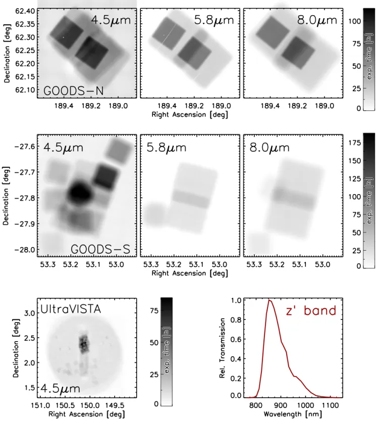
Our LF measurements are based on a composite sample of galaxies at4 z 7, selected in the rest-frame optical(z′band, leff ~0.9 mm ; see Figure1for its transmission efficiency), with the bulk of our sample formed by Lyman break galaxies(LBGs) from the CANDELS/GOODS-N, CANDELS/GOODS-S—ERS
fields. The z∼4 bin is complemented by a sample of galaxies from a catalog based on the UltraVISTA DR2 mosaics.
The LBG samples in the CANDELS GOODS-N/S and ERS
fields rely on the multi-wavelength photometric catalogs of Bouwens et al.(2015). These are based on the re-reduction of public HST imaging, and are enhanced by proprietary full-depth Spitzer/IRAC mosaics. Specifically, they benefit from novel full depth IRAC 5.8μm and 8.0μm mosaics, not available in the original catalog of Bouwens et al.(2015). The UltraVISTA DR2 catalog is based on the most recent publicly available mosaics at UV-to-NIR wavelengths (including UltraVISTA DR2 data sets), and complemented by an internal release of full-depthSpitzer/IRAC mosaics.
In the following sections, we briefly describe these two parent catalogs and detail the criteria we adopted to assemble ourfinal sample of galaxies.
2.1.1. GOODS-N/S and ERS
For this work, we adopted the catalog assembled by Bouwens et al. (2015) over the CANDELS/GOODS-N, CANDELS/GOODS-S, and ERS fields. Here, we briefly summarize the main features; the reader should refer to Sections 2 and 3 of Bouwens et al.(2015)for full details.
The catalog contains the photometry in the HST ACS F435W, F606W, F775W, and F850LP bands (hereafter indicated by B435,V606,i775 and z850), together with HST WFC3 F105W, F125W, and F160W(Y105,J125,H160)data from CANDELS (Grogin et al. 2011), and WFC3 F140W band
The catalog takes also advantage of full-depth mosaics in the fourSpitzerIRAC bands. The 3.6μm and 4.5μm mosaics were assembled by combining data from the IGOODS (PI: Oesch) and IUDF (PI: Labbé) programs with all the public archival data from either cryogenic or post-cryogenic programs over the GOODS-N and GOODS-S (GOODS, ERS, S-CANDELS,
position across each mosaic, enabling a more accurate flux measurement in the IRAC bands(see below). The mosaics in the 4.5, 5.8, and 8.0μm bands are key to this work, as they probe the rest-frame z′ band. Specifically, the 4.5μm band matches the rest-frame z′band at z∼4, whereas the 5.8 and 8.0μm bands are required for the rest-frame z′band atz5. Figure1 presents the exposure time maps in the IRAC 4.5, 5.8, and 8.0μm for the GOODS-N and GOODS-Sfields. As a result of the combination of data from different programs, the achieved depth across eachfield is highly inhomogeneous. This is particularly evident for the 4.5μm band, the depth of which ranges between 50 and 180 hr(corresponding to 25.1–25.8 AB, respectively, for 5s, 2 0 aperture diameter). The GOODS-N
field is characterized by the deepest 5.8 and 8.0μm data, reaching a depth of∼80 hr(∼24.5 AB,5s,2. 0 aperture).
The object detection was performed on thec2image(Szalay et al. 1999) constructed from theY105,J125,H160 band images. The detection mosaics have footprints of ∼124 and ∼140 arcmin2, respectively, for GOODS-N and GOODS-S, for a total of 264 arcmin2. Aperture photometry in the HST bands was performed in dual mode with SExtractor (Bertin & Arnouts 1996)on the mosaics matching the resolution of the
H160 image. Fluxes were converted to total through the application of an aperture correction based on the Kron
(1980) scalable apertures, and further corrected to take into account the flux losses of the scalable apertures compared to the PSF. Photometry of the IRAC mosaics was performed using a proprietary deblending code(Labbé et al.2006,2010a, 2010b, 2013). This code convolves the high-resolution HST
mosaics with a kernel obtained from the highest S/N IRAC PSFs, to construct a model of the IRAC image. For each object,
2. 0-diameter aperture photometry is performed on the image, which was previously cleaned from neighbors by using the information from the model image. The aperture fluxes were then corrected to total by using the HST template specific of each source, convolved to match theSpitzerIRAC PSF.
Candidate LBGs at z∼4, 5, 6, and 7 were selected from among theB435,V606,i775andz850dropouts, respectively. For a complete list of criteria adopted to select each sample, see Table 2 of Bouwens et al. (2015). The sample included 8031 LBGs.
2.1.2. UltraVISTA DR2
For the sample of z∼4 galaxies, we also considered detections in the COSMOS/UltraVISTA field, the relatively largerfield of which(compared to GOODS-N/S)allowed us to probe higher luminosities.
The UltraVISTA catalog used for this work is based on the
ultradeep stripes of the second data release (DR2) of the UltraVISTA survey (McCracken et al. 2012). This release is characterized by5s depth of∼25.6, 25.1, 24.8, 24.8AB (2. 0
aperture diameter)inY, J, H,andKs, respectively(~0.8 1.2– mag deeper than DR1), and extends over an area of ∼0.75 square degrees in four stripes over the COSMOS field(Scoville et al. 2007). The 37-band catalog was constructed following the same procedure presented in Muzzin et al. (2013a) for the DR1. Briefly, the detection was performed in theKsband; 33-band far-UV-to-Ksaperturefluxes were measured with SExtractor(Bertin & Arnouts1996)in dual mode, focused on the mosaics matching the PSF resolution of theH-band image. An aperture correction recovered from the Kron ellipsoid was applied on a per-object basis; total fluxes were finally computed by applying a further
aperture correction obtained from the PSF curve of growth. This new catalog also includes flux measurements in the Subaru narrow bands NB711, NB816, the UltraVISTA narrow band NB118, as well as the CFHTLSu∗,g¢,r¢,i¢, andz′, which are not available in the DR1 catalog of Muzzin et al.(2013a).
The COSMOSfield benefits from several hundreds hours of integration time withSpitzerIRAC. Similarly to what was done for the GOODS-N/Sfields, full-depth mosaics were constructed following the procedure of Labbé et al.(2015). Specifically, full depth 3.6 and 4.5μm mosaics were reconstructed by combining data from the S-COSMOS(Sanders et al.2007), S-CANDELS
(Ashby et al.2015) and SPLASH(PI: Capak, Steinhardt et al. 2014). The resulting coverage map for the 4.5μm band is shown in the lower panel of Figure 1. The depth ranges from∼4 to
∼90 hr, which corresponds to ∼23.8–25.4 AB (5s in a 2. 0
aperture).
Observations in the 5.8 and 8.0μm channels are only available from the S-COSMOS Spitzer cryogenic program. These data have a much shallower depth compared to the 3.6 and 4.5μm bands, with an average limit of∼22.2AB(5s, 2 0 aperture). For this reason, we only considered galaxies from the GOODS-N/Sfields for thez5samples.
Fluxes in the four IRAC bands were measured using the templatefitting procedure of Labbé et al.(2006,2010a,2010b, 2013), adopting the Ks band as the high-resolution template image to deblend the IRAC photometry.
Photometric redshifts were computed using EAzY(Brammer et al.2008)on the 37 bands photometric catalog, complementing the standard EAzY template set with a maximally red template SED, i.e., an old (1.5 Gyr) and dusty (AV =2.5 mag) SED
template. We only considered objects whose fluxes were not contaminated by bright nearby stars, with extended morphology on the Ks image. Less than five bands were excluded, as the associatedflux measurements were contaminated byNaNvalues. Galaxies in the z∼4 redshift bin were selected among those with photometric redshift 3.5<zphot<4.5. The initial z∼4
sample included 1208 objects.
The photometric redshift selection allowed us to consider objects that could have been missed by a pure LBG selection. The large area offered by the UltraVISTA DR2 footprint enabled the selection of bright/luminous sources whose surface density would be too low to be probed over the GOODS-N/S
fields area. Such luminous systems could be intrinsically redder than normal LBGs, either because they are more (massive) evolved systems and/or they contain a higher fraction of dust. On the other side, the LBG selection at fainter luminosities from the GOODS-N/S samples is expected to suffer only limited selection bias against intrinsic red sources, as galaxies in this range of luminosities are mostly blue star-forming systems, with low dust content.
2.2. Sample Assembly
Thefirst step consists of applying a cut in theKsflux of the galaxies from the UltraVISTA sample, in order to control the detection completeness. The DR2 data is∼1mag deeper than DR1. Therefore, we set the threshold to Ks=24.4 mag,
Successively, we excluded from our sample those galaxies with poor flux measurements in those IRAC bands used to compute the rest-frame z′ luminosity. The variation in depth across each IRAC mosaic prevented us from applying a single value offlux threshold at this stage. Instead, we applied a cut in S/N to theflux in the IRAC band closest to the rest-frame z′
band(i.e., IRAC 4.5μm atz∼4 and IRAC 5.8μm and 8.0μm atz5).
Considering the gap in the photometric depth probed by the 4.5μm mosaics compared to that reached by the 5.8–8.0μm data, we opted for applying a distinct S/N cut depending on the considered redshift bin. The sample at z∼4 was selected by applying the cut ofS N>5to the 4.5μmflux; the samples at
z∼5, 6, 7 were assembled by considering the cumulativeflux in the 5.8 and 8.0μm bands as the inverse-variance weighted sum of theflux in these two bands. We then applied a cut to the corresponding S/N such that:
º +
+ >
+ w w ( )
w w
S N5.8 8.0 S5.8 5.8 S8.0 8.0 4, 1
5.8 8.0
whereSkis theflux measurement in bandκandwκis the weight defined as1 sk2, withskthe correspondingflux uncertainty. The application of the S/N cut reduced the number of galaxies to 2644(2040/604 for GOODS/UltraVISTA, respectively), 96, 17 and 4 atz∼4,z∼5,z∼6, andz∼7, respectively.
We further cleaned our sample, excluding those objects satisfying any of the following conditions:(1)the contribution to the 5.8 and 8.0μm flux from neighboring objects is excessively high;(2)the source morphology is very uncertain or confused making IRAC photometry undetermined; (3) the source is detected at X-rays wavelengths, suggesting it is a lower redshift AGN;(4)the source is at higher redshift, but its SED is dominated by AGN light; (5) LBGs with a likely
<
z 3.5 solution from photometric redshift analysis. In Appendix A, we detail our application of these additional criteria in cleaning our sample.
Our final sample consists of 2098 galaxies at z∼4 (1680 from the LBG sample and 418 from the UltraVISTA sample), 72 at z∼5, 10 at z∼6, and 2 objects at z∼7. The distribution of the absolute magnitudes in the z′band for the sample is presented in Figure 2, for the four different redshift bins. It is noteworthy how the GOODS-N/S and UltraVISTA samples complement each other at z∼4, allowing to fully exploit these data with little redundancy.
2.3. Selection Biases
The samples adopted in this work rely on LBG selection criteria, complemented at z∼4 by a photometric redshift selected sample based on the UltraVISTA DR2 catalog.
The criteria adopted for the assembly of our samples introduce two potential biases to our estimates of LF, M* L
ratio and SMF(Fontana et al.2006; Grazian et al. 2015). The Lyman Break criteria select, by construction, blue star-forming galaxies, and may thus exclude a greater fraction of red objects compared to photometric-redshift selections. Furthermore, even samples based on photometric redshifts can suffer incomplete-ness from very red sources, too faint to appear in the detection bands (usuallyH or Ks or a combination of NIR bands), but that emerge at redder wavelengths (e.g., IRAC). In the following we attempt to evaluate the impact of these biases on our sample.
From the stellar mass catalog of CANDELS/GOODS-S
(Santini et al. 2015), we extracted those galaxies with photometric redshift3.5<zphot<4.5. Successively, we applied
the LBG criteria to their flux measurements from the multi-wavelength catalog of Guo et al.(2013). In Figure3we present, as a function of stellar mass, the ratio between the number of galaxies recovered through the LBG criteria and the number of galaxies in the photo-z sample. The plot shows that the LBG selection is able to recover75%of galaxies with stellar mass
* (M M )
log 10 (corresponding to ~-0.12dex offset in number density measurements); at log(M* M)10.5 the galaxies missed by the LBG criteria amount to about 35%
(∼0.2 dex). At higher stellar masses, the fraction of galaxies not entering the Lyman Break selection increases to 60% 70%– (~0.5 0.6– dex) consistent with Grazian et al. (2015). Duncan et al.(2014)showed that photometric uncertainties scatter a large fraction of the measurements outside the LBG selection box; specifically, the LBG criteria recover only~1 4(equivalent to ~-0.6dex offset) of the galaxies recovered through photo-z
(see also Dahlen et al.2010). However, once selection criteria on Figure 2. Distribution of the absolute magnitudes in the z′ band of our composite sample of galaxies atz∼4, 5, 6, and 7, as labeled in thefigure. For
the z∼4 sample, the histograms for the GOODS-N/S and UltraVISTA samples are also presented separately, showing the complementarity inMz¢of the two data sets.
Figure 3.Fraction ofz∼4 galaxies recovered using LBG criteria relative to the underlying sample of galaxies selected to have photometric redshifts
<z <
3.5 phot 4.5, shown as a function of stellar mass. The horizontal dashed
the redshift probability distribution are introduced, excluding from the sample poorly constrained photometric redshifts, the resulting photo-zsample largely overlaps with the LBG one, as demonstrated by the fact that the resulting photometric redshift UV LFs agree well, usually within1 -s, with the LBG UV LF
(Duncan et al.2014; Finkelstein et al.2015a).
The photometric depth of the UltraVISTA DR2 catalog, =
Ks 24.4mag, corresponds to a stellar mass completeness limit
for a passively evolving simple stellar population of * ~
(M M )
log 10.6 atz∼4 and 11.2 atz∼5. The depth in the GOODS-Deepfields correspond to limits in stellar mass of
* ~ (M M )
log 10.3 atz∼4 and 10.6 at z∼5, respectively. We would like to remark that our analysis for thez∼4 sample at stellar masses log(M* M)10 10.5– is dominated by the photometric redshift sample from UltraVISTA, covering a larger volume for bright sources than the GOODS fields. Therefore, our composite z∼4 sample is only marginally affected by the LBG selection bias.
A number of works have studied the so called extremely red objects, characterized by very red(2 3– mag)rest-UV/optical colors, making them more elusive in high-zsamples(e.g., Yan et al. 2004; Huang et al. 2011; Caputi et al. 2012, 2015; Stefanon et al. 2015; Wang et al. 2016). Samples detected in IRAC bands suggest that many of these objects could be consistent with being z3massive galaxies.
Recently, Wang et al. (2016) analyzed the properties of -[ ]>
H 4.5 2.25mag over the CANDELS/GOODS-N and GOODS-S fields. Interestingly they identified 18 sources not present in the H160-band catalog, but included in the IRAC catalog of Ashby et al. (2013). Of these, 5 sources have an estimated photometric redshift 3.5<zphot<4.5 and have a
stellar mass 10.5log(M* M)11. Since their analysis refers to the samefields we consider in our work(although likely the configurations at the detection stage are different), we can use their result to obtain a rough estimate of the fraction of objects missed by our selection. Assuming a M* Lz¢~0.2M L, quite typical for these masses and redshifts (as we show in Section 3.2), the stellar mass range of these galaxies would correspond to luminosities -24.7Mz¢-23.4 AB. This sample would then constitute~65% of the objects in ourz∼4 LBG sample with similar luminosities. This fraction drops to ~8%when comparing the 5 sources to the∼60 galaxies with the same photometric redshift and stellar mass over the CANDELS/ GOODSfields.
Caputi et al. (2015) presented SMF measurements at
~ –
z 3 5 obtained complementing the SMF from a photo-metric-redshift,Ks-selected sample based on UltraVISTA DR2 data to SMF measurements from photometric redshift samples ofKs-dropouts detected in IRAC bands. The main result is that
Ks dropouts can account for as high as ∼0.5dex in number densities. However, Stefanon et al.(2015)showed that samples similar to those of Caputi et al. (2015) likely suffer from degeneracies in the measurement of photometric redshifts(and consequently stellar masses), and therefore the above estimate is still uncertain.
The depth of current IRAC data, however, is not sufficient to systematically inspect passively evolving stellar population with stellar masses below~1010 10.5- Matz4. We therefore caution the reader that any sample currently available dealing with stellar mass below the~1010Mlimit may still be biased against dusty and/or old galaxies. Forthcoming projects, like
Spitzer/GREATS(I. Labbé et al. 2017, in preparation)and the
JWST will allow us to obtain a more complete picture by probing the lower mass regime.
2.4. Selection Efficiency and Completeness
We implemented a Monte Carlo simulation based on real data to estimate the effects that our selection criteria in S/N and contamination polishing have on the sample of galaxies used in this work. For this simulation, we did not consider the effects of selection in the detection band, because the UltraVISTA sample is 90% or more complete in Ks by construction, whereas the effects of detection completeness in the GOODS-N/S sample have been taken into account when estimating the co-moving volumes adopted for the LF measurements.
We first defined a grid in apparent magnitude of width 0.20mag. Given the small sizes of the galaxies compared to the IRAC PSF, for each magnitude value in the grid, we injected 100 point sources randomly distributed across a region of uniform depth in the 4.5, 5.8, and 8.0μm mosaics of the GOODS-Nfield. We chose the GOODS-N because thisfield is characterized by the deeperSpitzer/IRAC 4.5, 5.8, and 8.0μm band data among the fields considered for this work. We successively replicated the flux measurement, using the same procedure adopted for the actual photometry.
The completeness fraction in each magnitude bin was computed by comparing the number of objects satisfying our selection criteria(Section2.2)to the number of objects initially injected into the simulation. For the completeness of thez∼4 sample, the above process was applied to the 4.5μm mosaic only. For the completeness of the samples atz5, the point sources were added at matching positions in the 5.8 and 8.0μm mosaics. The selection of the S/N and contamination was then recovered by applying the corresponding criteria and assuming the SED to beflat infνin the observed 5–9μm region. This is a reasonable approximation because, as we show in Section3.2, the median SEDs do not substantially deviate from a flat fν
SED in the wavelength range covered by IRAC observations. The whole process was repeated10´in each band, to increase their statistical significance. The global completeness (i.e., the cumulative effects of S/N and contamination selection)at the different depths of the IRAC mosaics was obtained by rescaling the completeness in S/N selection to match the depth of the relevant region.
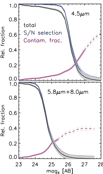
The results from our completeness simulation for the 4.5μm and the 5.8μm+8.0μm samples are presented in Figure 4. Wefirst discuss the recovery of the contamination fraction; we then consider these results in the budget of our global completeness estimates.
The fraction of objects in the 4.5μm band contaminated by neighbors6is negligible for objects brighter than∼24AB, and increases exponentially up to∼27AB, where it starts toflatten out. A similar behavior is observed for the 5.8μm+8.0μm simulation, although shifted at brighter magnitudes due to the shallower depth of the 5.8 and 8.0μm compared to the 4.5μm. The flattening at the faint end is caused by a strong incompleteness in the data at such faint magnitudes, and likely does not reflect the true behavior. In what follows and our analysis, we do not consider the completeness for magnitudes fainter than those corresponding to the onset of the flattening,
6
i.e.,∼27AB and∼25AB for the 4.5μm and 5.8μm+8.0μm data, respectively.
As it could intuitively be expected, the bright end of the global completeness curve is dominated by the (small) fraction of purged objects. This effect becomes less and less pronounced at fainter magnitudes, corresponding to lower S/N, where the effective selection is driven by the S/N itself.
2.5. Flux Boosting
The random noise from the background can positively combine at the location of a given source, introducing an increase in the measuredflux(flux boosting, Eddington1913). The amount of this boost is inversely correlated to the S/N of the source. Theflux for sources with very high S/N will mostly be the result of the photons emitted by the source itself, with reduced contribution from the background; on the other hand, for sources with low S/N, the background level can be
typically just few factors smaller than the intrinsic signal from the source, making it sensitive to(positive)fluctuations of the background. Furthermore, sources do not uniformly distribute with flux, but rather follow an approximate power law, with fainter sources more numerous than brighter ones. Therefore, it is intrinsically more probable that fainter sources scatter to brighterfluxes than the reverse, giving origin to a netflux bias. A second potential source of flux boosting comes from confusion noise: faint sources at apparent positions close to a brighter one are more likely to be blended into the brighter source, increasing theflux and decreasing the number of fainter objects. This effect is larger for flux measurement in those bands with wide PSF, like Spitzer/IRAC. However, in our case, the photometry in the IRAC bands was performed by adopting a higher-resolution morphological prior from HST
mosaics(see Section2.1). Furthermore, we applied a selection in flux contamination (see Section 2.2). Because these two factors drastically limit the potential contribution of confusion noise to the IRAC fluxes in our sample, we do not further consider its effects to theflux-boosting budget.
For each source, we estimated the flux bias as the ratio between the expected intrinsicfluxfiand the measuredfluxfo. Because no direct measurement is possible, the intrinsic flux was recovered as the averageflux obtained from an estimate of its probability distribution. This was constructed considering two distinct contributions:(1) the probability(f fi, o)that the
observedfluxfois drawn from the distribution of intrinsicfluxfi, given the noiseso, and (2) the frequency( )fi of occurrence of the intrinsicfluxfi. Assuming each probability is normalized to 1, the final probability distribution would then be tot( )fi =
(f fi, o) ( ) fi . 7
Assuming a Gaussian noise,(f fi, o)can be written as:
ps s
= -
-(f f, ) 1 [ (f f ) ] ( ) 2
exp 2 , 2
i o
o
i o o
2
2
normalized to a total probability of one.
The frequency associated with the intrinsic flux can be recovered from the (intrinsic) differential number count of sources,dN f( )i dfi. This can usually be described by a power-law form with negative index, which is thus divergent for
fi 0, preventing it from being normalized
8(see, e.g., Hogg & Turner 1998, who also discuss possible reasons why the divergence at fi 0 is likely non-physical).
We therefore followed the formalism of Crawford et al.
(2010), who introduced, as further constraint, the Poissonian probability that no sources brighter than fi exist at the same location of the observed object. The expression for( )fi then becomes:
= ´ ⎛-DW
ò
+¥⎝
⎜ ⎞
⎠ ⎟
( )f dN f( ) ( )
df exp dN df , 3
i
i
i
o fi
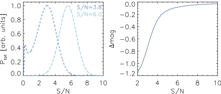
whereDWocorresponds to the area occupied by the source. In the left panel of Figure5, we show examples of reconstructed
( )tot, for the cases of S/N=6 and S/N=3.8, where it is evident that the contribution of the faint source population to Figure 4.Completeness fraction as a function of apparent magnitude, from our
Monte Carlo simulation for selection of the 4.5μm (top panel) and 5.8μm+8.0μm(bottom panel)bands. The pink curve presents the fraction of objects excluded because theirflux measurements were highly contaminated by neighbors. The pink shaded area presents the associated 1s Poisson uncertainties. The blue curve and shaded area present the completeness fraction from the S/N cut in theflux of the corresponding band and associated Poisson uncertainty, respectively. The black curve and gray shaded area show the combined effect of S/N threshold and contamination cleaning, respectively.
7
A similar expression could also be recovered, modulo a normalization factor, by applying Bayes’theorem—see, e.g., Hogg & Turner(1998). 8
For S/N5, the product of (f fi, o) and dN/df does not diverge for
fi 0. However, this is no longer the case for lower S/N values, where the
the expected intrinsicflux increases as the S/N decreases. The right panel of Figure 5 shows the expected flux boost as a function of S/N. ForS N4.5, theflux boost is roughly the same amount as theflux uncertainty. However, for lower S/N, the estimatedflux boost increases abruptly. For S/N2, the expectedflux boost is1.5mag, meaning that the recovery of the intrinsic flux for such low S/N data is highly uncertain.
The S/N in theHSTbands for the galaxies in our sample is >10. At z∼4, the S/N in the 4.5μm band, adopted for the selection of thez∼4 sample, is5by construction; the S/N in the 3.6μm band is5as well, consistent with the nearlyflat SEDs in that wavelength range. At z5, the selection was performed in a combination of 5.8μm and 8.0μm fluxes, adopting a S N >4 threshold. Figure 5 shows that the expected flux boost forS N >5 is0.1mag. However, for lower S/N, typical of the selection of samples at z5, the correction can be as high as ∼0.8–1.0 mag.
We therefore applied the above correction to thefluxes in the 5.8 and 8.0μm of thez5 samples. The averageflux boost was ∼0.19mag and ∼0.25mag in the IRAC 5.8μm and 8.0μm bands, respectively.
In Appendix B, we present the SEDs of the 12 most luminous galaxies in thez∼5 sample, along with the SEDs of thez∼6 andz∼7 samples, before and after applying theflux boost correction.
3. Results
3.1. UV to Optical Luminosities
In the last few years, a number of works have studied the relation between the rest-frame UV luminosity and the stellar mass of high-redshift galaxies(e.g., Stark et al.2009; González et al.2011; Lee et al.2011; McLure et al.2011; Duncan et al. 2014; Spitler et al.2014; Grazian et al.2015, V. González et al. 2017, in preparation; Song et al. 2016). Indeed, a relation between the stellar mass and the UV luminosity is to be expected when considering a continuous star formation. Devia-tions from such a relation would then provide information on the
age and metallicity of the stellar population and dust content of the considered galaxies.
The emerging picture is that, atz∼4 and for stellar masses
* (M M )
log 10, the stellar mass increases monotonically with increasing UV luminosity; however, at stellar masses higher than log(M* M)~10, the trend becomes more uncertain: Spitler et al. (2014), using a sample of Ks-based photometric redshift selected galaxies, found indication of a turnover of the UV luminosity, with the more massive galaxies
(10.5log(M* M)11) spanning a wide range in UV
luminosities(see also Oesch et al.2013). Lee et al.(2011), on the other hand, using an LBG sample, found a linear relation between UV luminosities and stellar masses up to
* ~ (M M )
log 11. Considering the different criteria adopted by the two teams for the assembly of their samples, selection effects might be the main reason for the observed tension.
This observed discrepancy could, however, just be the tip of the proverbial iceberg. Indeed, current high-z surveys might still be missing lower-mass, intrinsically red galaxies (dusty and/or old), which could populate the M*–MUV plane outside the main sequence(Grazian et al.2015 and our discussion in Section 2.3). The depth of the current NIR surveys does not allow us to further inspect this, which will likely remain an open issue untilJWST.
A monotonic relation between the UV luminosity and the stellar mass has also been found at z∼5 and z∼6 for
* (M M )
log 10 (e.g., Stark et al. 2009; González et al. 2011; Duncan et al. 2014; Salmon et al. 2015; Song et al.2016), with approximately the same slope and dispersion, but with an evolving normalization factor(but see, e.g., Figure 5 of Song et al.2016for further hints as to the existence of massive galaxies with faint UV luminosities).
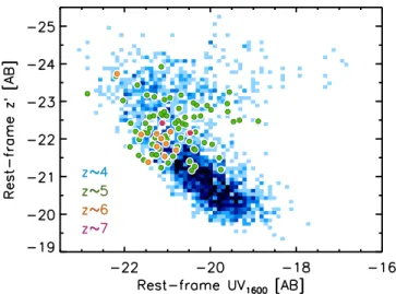
Figure6presents the absolute magnitude in the rest-framez′
band(Mz¢)as a function of the absolute magnitude in the UV
(MUV1600), for our sample in the four redshift bins(z∼4, 5, 6 and 7). In Figure 7, we present the binned median in the
¢
–
MUV Mz plane for the z∼4 andz∼5 samples.
Figure 5.Left panel: examples of probability distribution of the intrinsicflux( )fi, presented as a function of S/N, for two cases of observed S/N=3.8 and 6.0, as
The z∼4 sample shows a clear correlation between the luminosities in the rest-frame UV andz′bands forMz¢-22 mag, which can be described by the following best-fitting linear relation:
= -( )+( )´ ¢ ( )
MUV 3.58 1.49 0.79 0.07 Mz. 4
The above bestfit is marked by the magenta line in Figure 7, where we also indicate the 3s limits corresponding to our 5.8μm+8.0μm selection. At z∼4 andz∼5, the depth of the IRAC data allows us to not only probe the bright end, where the relation between MUV and Mz¢ breaks, but to also explore the regime of the linear correlation expressed by Equation (4). Slopes of 0.4–0.5 in the log(M*)–MUV plane
(with nominal 1s uncertainties of ~0.05 0.1)– have been reported by, e.g., Duncan et al. (2014) and Song et al.
(2016). Assuming a constantM* Lz¢ratio(see Section3.2), our measurements correspond to a slope of 0.5 in thelog(M*)–MUV plane, consistent with previous measurements.
Assuming that the SFR mostly comes from the UV light, and thatMz¢is a good proxy for stellar mass measurements, we can also compare the slope we derived for the MUV–Mz¢relation to that of the log(SFR)–log(M*) from the literature. Indeed, the observed UV slopes of Mz¢-22 galaxies in our sample are
b~ -2 (see also Bouwens et al. 2010), consistent with star-forming galaxies and little-to-no dust extinction. Our measure-ment is perfectly consistent with the log(SFR)–log(M*)slope of ~0.80.1recently measured by, e.g., Whitaker et al. (2015) for z2.5 star-forming galaxies with log(M* M)10.5, and it has been shown to evolve little over the redshift range0.5< <z 2.5.
For absolute magnitudes brighter than Mz¢~ -22mag, the linear relation expressed by Equation(4)breaks as we observe the beginning of a turnover in the absolute UV–z′ magnitude relation. Remarkably, this behavior is visible also for thez∼5 sample, which is entirely based on LBG selection. This fact has important consequences for, e.g., SMF measurements; samples of galaxies selected at fixed rest-frame UV luminosity are potentially characterized by a wide range of stellar mass.
The absolute UV magnitude of galaxies withMz¢~ -23.5
0.8mag spans the full range of values observed for
-¢
Mz 22.5 mag. However, the bulk of values aggregates
around the[MUV,Mz¢]~ -[ 21.4,-23.5]mag region, and it is characterized by a large dispersion in MUV (3 mag). This result is qualitatively consistent with the findings of Spitler et al. (2014), assuming a correlation between the absolute magnitudeMz¢and the stellar mass. Most of the galaxies with
~ -¢
Mz 23.5 come from the photometric redshift sample
selected from the UltraVISTA catalog. As we will present in Section 3.2, our measurements of the mass-to-light ratios from stacking analysis show that galaxies with Mz¢-23.5 statistically have stellar masses log(M* M)10.6. The above result then underlines the bias that LBG selections may introduce against massive systems.
Atz∼5, our data allow us to inspect the relation only for ¢
Mz fainter than−23 andMUV,1600 fainter than~-22. In this range of luminosities, our z∼5 measurements are roughly consistent with the z∼4 measurements in the same range of luminosities. The measurements for the z∼6 and z∼7 samples are still consistent with the trends observed atz∼4, although the low number of objects does not allow us to derive any statistically significant conclusion.
3.2. Stellar Mass-to-light Ratios from Stacking Analysis
Thus far, determinations of the stellar mass-to-light ratios
(M* L)for galaxies atz>4have involved theM* LUVratio. This quantity is fundamental to our understanding of galaxy formation and evolution, as it combines information on the recent (through the UV luminosity) and integrated (through the stellar mass)SFH(e.g., Stark et al.2009). Nonetheless, the
*
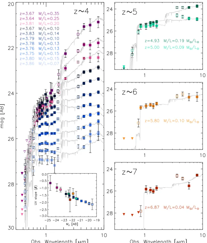
M LUVhas been used to recover the stellar mass and SMF of high redshift galaxies with alternating success (see, e.g., González et al. 2011; Song et al. 2016). In this section, instead, we explore for the first time the M* Lz¢properties of galaxies at z4. The rest-frame z′ luminosity is more sensitive to the stellar mass, compared to the UV luminosity, for two reasons. Although the UV light is emitted by massive, short-lived stars, and thus traces the SFH in the past few hundred Myr, the luminosity in the rest-frame optical region mostly originates from lower-mass, longer-lived stars, which Figure 6. The z′absolute magnitudes vs. UV absolute magnitudes for our
composite sample, color-coded according to the considered redshift bin. The
z∼4 data are presented as a density plot, with denser regions identified by a darker color, whereas the points for thez5samples are shown individually. The UV–z′relation shows a turnover forMz¢-22.5.
Figure 7.Median of theMUVvs.Mz¢relation in bins ofMz¢. The blue points
constitute most of the stellar mass of galaxies. Furthermore, it is less sensitive to the dust extinction, and hence to the uncertainties in its determination, compared to the UV; for a Calzetti et al. (2000) extinction curve, an AV=1 mag gives
~ l
A1600 2.5mag, compared to Al9000 ~0.5mag.
Because we are interested more on average trends in the * ¢
M Lz ratios here, rather than studying it for specific galaxies, we performed our analysis using the median stacked SEDs constructed from our composite sample. Due to the different photometric bands in the catalogs, we performed the stacking of sources separately for sources in the GOODS-N/S and UltraVISTA samples.
The stacked SEDs were constructed as follows (see also González et al.2011). At each redshift interval, we divided the galaxies into sub-samples according to their Mz¢. The different depths reached by the 4.5μm and 5.8μm+8.0μm samples resulted in different numbers of subsamples across the redshift bins. Under the working assumption of limited variation in both redshift and SED shape in each bin ofMz¢, as well as for each
HST band, we took the median of the individual flux measurements. Our assumption is also supported by the fact that the SEDs from stacking are generally characterized by a
flatfν continuum at both rest-frame UV and optical regimes. Uncertainties on the median were computed from bootstrap techniques, drawing with replacement the same number offlux measurements as the number of galaxies in the considered absolute magnitude bin. Before median-combining, thefluxes were perturbed according to their associated uncertainty. The process was repeated 1000 times, and the standard deviation of the median values was taken as the final uncertainty. For the IRAC bands, median stacking was performed on the mosaic cutouts centered at the position of each source, previously cleaned from neighbors. Photometry was performed on the median of the images in apertures of2. 5 diameter. Totalfluxes were then recovered through the PSF growth curve. Uncer-tainties were computed by applying to the image cutouts the same bootstrap technique adopted for the median stacking of thefluxes, as described above. In randomly drawing the image cutouts, we preserved the total exposure time.
Photometric redshifts andz′-band luminosities were obtained from EAzY (Brammer et al. 2008) on the stacked SEDs. Briefly, EAzY initially selects the two SED templates that provide the closest match to the observed color in the two
filters bracketing the rest-frame band of interest. The luminosity is then computed from the interpolation of the two colors, relative to the rest frame band of interest, obtained from the two selected SEDs(for full details, see Appendix C of Rudnick et al.2003). Stellar masses were computed by running FAST (Kriek et al. 2009), adopting the Bruzual & Charlot
(2003) template SEDs, a Chabrier (2003) IMF, solar metalli-city, and a delayed-exponential SFH. The bands potentially contaminated by nebular emission were excluded from thefit. Because we performed the stacking in each band individually, assuming the same redshift for all sources, the flux in those bands close to the Lyman and the Balmer breaks potentially suffers from high scatter introduced by the range of redshifts of the galaxies in each sub-sample, depending on whether the break enters the band. Fluxes in these bands were therefore excluded from the fit with FAST. Specifically, for the z∼4 LBG stacks, we excluded theB435,V606andH160bands; for the
z∼4 UltraVISTA stacks, we excluded the B, IA427, IA464, IA484, IA505, IA527, IA574, IA624, IA679, g g¢, +,V H,
bands; for thez∼5 stacks, we excluded theV606and the i775 bands; for thez∼6 stack, we excluded thei775band; for the
z∼7 stack, we excluded the I814 band. The stacked SEDs, along with the best-fit templates from FAST, are presented in Figure8.
The photometric redshifts measured from the stacked SED are all consistent with the values of the corresponding redshift bin; the difference of the photometric redshifts of the median stacked SEDs and the median of the photometric redshifts of the individual sources in each subsample is Dz (1+z)0.05, i.e., within the uncertainties expected for photometric redshifts. The inset in the left panel of Figure8presents the slope of the UV continuum(β), measured on the stacked photometry, as a function of absolute magnitude Mz¢. The stacked SEDs at
z∼4 andz∼5 are characterized by a trend in the UV slope, with bluer slopes for low-luminosity galaxies, particularly evident for the z∼4 stacks, and qualitatively consistent with the results of, e.g., González et al. (2011) and Oesch et al.
(2013). Our measurements do not present evidence for evolution of β with redshift at fixed luminosity (»M*), although the large uncertainties inβ (especially for the higher redshift bins)may be blurring trends. Furthermore, the SEDs in the rest-frame UV wavelength region of the four or five brightestz∼4 stacks do not differ too much one from each other, whereas they differ substantially at wavelengths redder than the Balmer/4000Åbreak.
Recently, Oesch et al. (2013) presented stacked SEDs at
z∼4 in bins ofz-band absolute magnitudes from a sample of galaxies based on CANDELS/GOODS-S, HUDF, and HUDF09-2. The sample benefits from deep IRAC 3.6μm and 4.5μm imaging from the IUDF program. The stacked SEDs (see, e.g., their Figure 2) show a clear trend of redder colors with increasing rest-frame z-band luminosity, in particular forMz< -21.5. Our stacked SEDs are in qualitative
agreement with those of Oesch et al. (2013), confirming the observed trend with luminosity. Furthermore, thanks to the wide area offered by UltraVISTA, which provides coverage for even brighter sources, we are able to extend the trend to even more luminous galaxies.
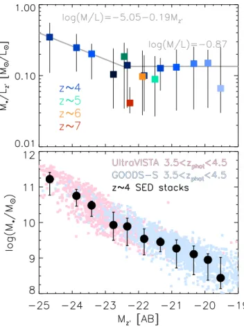
In the top panel of Figure 9, we present the M* Lz¢ measured9from the stacked SEDs as a function ofz′absolute magnitude. Total uncertainties were obtained by propagating the 68% confidence intervals in stellar mass generated by FAST and the uncertainties in luminosity, taken as the flux uncertainties from stacking. At z∼4, the M* Lz¢ ratio is consistent with being constant for Mz¢ fainter than ~-22.5 mag. Wefind:
* ¢ = - ¢
-(M L ) M ( )
log z 0.87 0.09, for z 22.5. 5
ForMz¢-22.5mag, there is indication ofM* Lz¢increasing with the luminosity, although the error bars are large. The
best-fit SEDs of the most luminous stacks have a nearly constant age
(~108.8 yr), and show an A
V slightly increasing with stellar mass (from 1.0 to 1.2 mag). A linear fit of the log(M* Lz¢)
values forMz¢-22.5mag resulted in the following relation:
* = - - ´ -¢ ¢ ¢ ( ) ( ) ( ) ( )
M L M
M
log 5.1 4.7 0.19 0.18 ,
for 22.5. 6
z z
z
9
Our linear relation recovers a constant value oflog(M* Lz¢)= -0.87 at Mz¢~ -22.5. However, the uncertainties on the fit parameters make the above relation also consistent with a constant value.
thez∼7 sample only includes two sources, thus reducing the statistical significance of the observed disagreement.
The above results are consistent with what is observed in Figure6. In Section3.1, we showed that galaxies more luminous than Mz¢~ -22.5mag form a cloud in the rest-frame UV–z′ plane around MUV~ -21.4mag. From our stacking analysis,
the average apparent magnitude atlobs~8000Å(i.e., the
rest-frame UV1600)for the stacked SEDs with[4.5 mm ]<23.5AB is
∼24.7AB, which corresponds atz∼4 to an absolute magnitude ~
-MUV,1600 21.4. According to the above relation, the stellar
mass corresponding toMz¢~ -23mag islog(M* M)~10.3. This behavior raises concern about potential biases that can occur when adopting the UV luminosity and M* LUV in the measurement of stellar masses, particularly for massive galaxies. A constantM* L is equivalent to a slope of−0.4 in the log
(stellar mass)—absolute magnitude plane. Our result atz∼4, obtained for galaxies with Mz¢< -23mag, is consistent with the~-0.4slopes found in the stellar mass—MUVplane (see, e.g., Duncan et al.2014; Grazian et al.2015). Steeper slopes,
such as those found by Stark et al. (2009), González et al.
(2011), Lee et al.(2011), McLure et al.(2011), and Song et al.
(2016), require thelog(M* L)to decrease for fainter galaxies, increase for brighter galaxies, or a combination of both effects. The origin for this is still unclear, as it could be a mix between selection effects (see, e.g., Grazian et al. 2015) and nebular emission contamination, which could boost the stellar masses of the more luminous galaxies(e.g., Song et al.2016).
In the bottom panel of Figure9, we compare the measure-ments of stellar mass and luminosity recovered from our stacking analysis to acontrolsample. This sample is composed of individual measurements selected from the COSMOS/ UltraVISTA and CANDELS/GOODS-S catalogs to have photometric redshifts3.5<zphot<4.5.
The individual measurements of the control sample distribute according to a monotonic relation defining a main sequence, with a scatter of about∼0.7dex. This correlation holds over a wide range of values, both in stellar mass and luminosity. In particular, we notice the absence of any turnover, as instead is observed when consideringMUV–M*, e.g., Spitler et al.(2014)
or equivalently, our Figure6. Furthermore, there are virtually no measurements outside the main sequence.
The relation between the stellar mass and luminosity recovered from the stacking analysis is in excellent agreement with the values of the control sample. We remark here that the control sample was selected based exclusively on photometric redshifts criteria. The agreement between our stacking results in the GOODSfield, then, indicates that the stacking does not suffer any major bias from the LBG selection. This result is not unexpected, however, given the low fraction of objects missed by the LBG selection for stellar masseslog(M* M)10.2, as we showed in Section2.3.
Together, these two results increase our confidence in the reliability of thez′band as a proxy for the stellar mass, s well as the robustness of our stacking analysis.
3.3. Evolution of the z′-band Luminosity Function
The LFs were measured adopting the 1 Vmax estimator
(Schmidt1968). Although this method is intrinsically sensitive to local overdensities of galaxies, the clustering is expected to be negligible atz>4. On the other hand, the1 Vmax method directly provides the normalization of the LF. Furthermore, and most importantly, the coherent analysis extension developed by Avni & Bahcall(1980)is key to this work.
As we showed in Section2.1, our composite sample is based on a dual-bandflux selection, corresponding to a doubleflux threshold. The detection process introduces thefirstflux cut in the corresponding band (Ks or c2 image built from the HST NIR bands, for the UltraVISTA and GOODS-N/S sample, respectively). The S/N cut on theflux in the IRAC band closest to the rest-framez′is responsible for the secondflux threshold in the relevant IRAC band.
For each galaxy in the sample, eachflux threshold generates an upper limit to the redshift the specific galaxy can have and still be included in the sample. These different upper limits in redshift correspond to different comoving volumes for each object that could potentially enter the Vmax computation. The coherent approach allowed us to take this double selection into consideration in a consistent way: the upper limit in redshift, used to compute the comoving volume, was taken to be the smaller of the two redshift upper limits, computed based on the threshold in the corresponding selection band. Furthermore, as Figure 9.Top panel: the color-filled squares with error bars present the
we showed in Figure 1, the depth of the IRAC mosaics is highly inhomogeneous. Therefore, for the computation of the comoving volumes in each field, we divided the IRAC footprint into a number of sub-fields, such that each sub-field was characterized by nearly homogeneous depths in both the detection10 and relevant IRAC band. Again, the Avni & Bahcall (1980) prescription allowed us to coherently analyze the different sub-samples.
Comoving volumes were computed differently, depending on the field and on the band driving the selection. For the galaxies in the GOODS-N/S fields, we used the comoving volumes computed by Bouwens et al. (2015). These volumes were estimated using an extensive Monte Carlo simulation based on real data. Sources were added to the different mosaics and recovered following the same procedure applied for the assembly of the LBG sample. Such volume estimates natively take into account the selection effects at the detection stage, and correct for flux-boosting effects and contamination by lower redshift interlopers and brown dwarfs. The volumesVifor those objectsiin the GOODS-N/Sfields whose redshift upper limit
zup was driven by the IRAC S/N threshold (zup ºzup,IRAC) were rescaled by the ratio between the volume associated with the redshift upper limit of the IRAC bandV zi( up,IRAC)and that
of thec2 image c
( ) V zi up, 2:
= ´
c
( )
( ) ( )
V V V z
V z . 7
i i i i ,IRAC ,GOODS up,IRAC up, 2
For the UltraVISTA sample, the volumes were computed directly from the limits in redshift that correspond to the flux limits in theKs and 4.5μm bands.
We computed the LF in four redshift bins centered atz∼4,
z∼5, z∼6, andz∼7. Although the IRAC data potentially allowed us to consider galaxies at z∼8, we did notfind any candidate with reliable flux measurement in the IRAC 5.8 and 8.0μm. Uncertainties on the LF measurements were derived by combining in quadrature the Poisson noise in the approx-imation of Gehrels (1986) to an estimate of cosmic variance from the recipe of Moster et al. (2011). The average cosmic variance value obtained for thez∼4 UltraVISTA sample was
∼0.43; the average cosmic variance estimates for the GOODS-N/S sample were~0.27,~0.41,~0.58, and ∼0.80, respec-tively, for the z∼4, 5, 6, and z∼7 redshift bins. The high values of the cosmic variance registered for all redshifts and luminosities are the dominant source of stochastic uncertainties in our LF measurements.
Our LF measurements are presented in Figure 10 and Table1. The LF atz∼7 consists of a single-bin measurement, and is characterized by large uncertainties that do not allow us to properly constrain its shape. The absolute magnitude range of the z∼4 LF spans ∼5 magnitudes, 3´more than the magnitude range of the z5 LFs. The larger absolute magnitude range available at z∼4 is the result of a number of distinct factors. First, the increased depth in the 4.5μm band from the combination of Spitzer/IRAC cryogenic and post-cryogenic epochs enables us to reach fainter absolute magnitudes than the cryogenic 5.8+8.0 mm data alone at
z 5. Second, the smaller PSF size of the 4.5μm data, compared to the 5.8μm and 8.0μm bands, allows to reach
fainter fluxes for the same exposure time and detector efficiency. Third, the availability of COSMOS/UltraVISTA data over an area~ ´4 larger than the GOODS-N/S footprint allowed us to recover the exponential decline of the bright end of thez∼4 LF, which is otherwise inaccessible by the small footprint of the GOODS-N/S mosaics.
In order to verify the consistency of thez∼4 LF with respect to the GOODS-N/S and UltraVISTA data, we also computed the LF separately on each one of these two data sets. The resulting LFs are marked in Figure10by the open squares, and show a good agreement with the LF from the composite sample.
The large uncertainties associated to the number density measurements atz∼5, 6, and 7 do not allow us to disentangle whether the evolution is in luminosity, number density, or both. In Section 3.5, we attempt to analyze this in a more quantitative way.
The dashed gray curve in Figure10marks thez~0 LF of Kelvin et al.(2014), measured with data from the Galaxy and Mass Assembly (GAMA) survey (Driver et al. 2009). Com-pared to our lowest redshift LF measurement, thez~0LF is characterized by a steeper decay for Mz¢-24.5. Fully
understanding the evolution of the LF from z∼4 to z~0
goes beyond the scope of the present work. However, qualitatively, a decrease in luminosity at z~0 compared to
z∼4 is expected, considering the lower values of the star formation rate density atz~0 than atz∼4 (e.g., Madau & Dickinson2014), and that thez′band may retain the effects of the recent SFH. This is particularly true for the bright-end of the LF: indeed, the brightest(i.e., most massive)galaxies that are still forming stars at z∼4 are likely to become quenched byz~0 (e.g., Muzzin et al.2013b).
3.4. Evolution of the SMF
We generated SMF measurements by taking advantage of the mass-to-light ratios we measured in Section 3.2. The fact thatM* Lz¢does not decrease with luminosity makes the shape of the LF resemble that of the SMF, allowing us to attempt a simple and straightforward conversion of the LF into the SMF. OtherM/L relations allow for the recovery of the SMF from the LF, although in a less straightforward way. We further discuss this in Section4.1.
We adopt the following very simple procedure. We assume that the constantlog(M* Lz¢)and the linear relation observed at
z∼4 (Equations (5) and (6)) are valid at all redshifts. The absolute magnitudes corresponding to the bin centers of the LFs are converted into stellar mass by applying the relevant
* ¢
(M L )
log z relation, depending on the Mz¢ value (see Equations(5)and(6)). We then differentiate the two relations, solving fordM*. The obtained values, specific for eachM*bin are used to rescale the LF normalization, to take into account the change in units from mag−1to dex−1.
Our SMF measurements are presented in Figure 11 and Table 2. Unsurprisingly, the z∼4 SMF covers a range in stellar mass wider than thez∼5, 6, and 7 SMFs, for the same reasons we described for the LF.
In Figure 11, we also plot a compilation of SMF measurements from the literature(Pérez-González et al. 2008; Marchesini et al. 2009, 2010; Stark et al. 2009; González et al. 2011; Lee et al. 2012; Santini et al. 2012; Ilbert et al. 2013; Muzzin et al.2013b; Duncan et al.2014; Stefanon et al. 2015; Caputi et al.2015; Grazian et al.2015; Song et al.2016; Davidzon et al. 2017). Atz∼4, starting from the low-mass
10
Because it is not straightforward to associate a limiting magnitude with a
c2image from the combination of differentfilters, we considered WFC3/H
end where the measurements are generally quite consistent with each other, the discrepancies increase with increasing stellar mass. One possible reason for the increased dispersion at higher masses is that galaxies constituting the low-mass end are mostly star-forming. Their redshift can then be assessed through the location of the observed Lyman break(either from dropouts or photometric redshift selections). The massive end, instead, possibly also includes more evolved and/or dusty systems, and it is therefore more sensitive to the degeneracy in identifying the observed break as either the Balmer/ 4000Åbreak or the Lyman break.
Ourz∼4 SMF determination is in good agreement with the SMFs of Stark et al. (2009), Lee et al. (2011), Stefanon et al.
(2015), Caputi et al.(2015), Grazian et al.(2015), Song et al.
(2016), and Davidzon et al. (2017). This is quite remarkable, because these SMFs have been recovered from different selection techniques. Specifically, Stark et al. (2009) and Lee et al. (2011) have measurements based on dropouts samples fromHST/WFC3 data; the SMF of Grazian et al.(2015)was built from aH160-detected photometric redshift sample over the CANDELS/GOODS-S and CANDELS/UDSfields; Stefanon et al.(2015)assembled a composite sample that complements a
Ks-detected catalog from UltraVISTA data with detections in IRAC 3.6 and 4.5μm bands; Caputi et al. (2015) use measurements based on aKs-detected SMF complemented by SMF measurements from detections in IRAC 4.5μm. The sample selection of both Stefanon et al.(2015)and Caputi et al.
(2015)relies on photometric-redshift measurements. Song et al.
(2016)recovered the SMF measurements by converting the UV LF into SMF through a linear M*–MUV relation for
*<
M 1010M , complemented by bootstrapped estimates at
*>
M 1010M . Finally, the SMF of Davidzon et al.(2017)was
based on a photometric-redshift sample from Ks-detection in COSMOS/UltraVISTA DR2 mosaics. On the other side, the
normalization of our SMF is higher than González et al.(2011) SMFs; these measurements were obtained by converting the observed UV LF into SMF through M* LUV measurements. The discrepancy between our SMF (and the bulk of the other SMF determinations) could be due to a steeper M* LUV relation found by González et al.(2011), and consequent lower normalization term.
At the massive end (log(M* M)11.2), we observe a discrepancy between our z∼4 SMF and some of the corresponding measurements from the literature (e.g., Ilbert et al.2013; Muzzin et al. 2013b). This discrepancy could, at least in part, be explained by our SMF lacking any scatter in
* ¢
M Lz for a givenLz¢. Our stacking analysis, by construction, recovers median M* Lz¢ ratios, potentially excluding such extreme cases as very dusty/old systems with very high stellar masses. However, the bottom panel of Figure 6, and our discussion in Section2.3, show that our sample is not strongly biased against this class of objects in the limits of current data. Nonetheless, they do not allow us to properly ascertain their existence at lower stellar masses. Aside from that, because of the Eddington bias, a distribution in the observed M* Lz¢ values for a specific luminosity would introduce a higher fraction of lower stellar mass objects that are scattered to higher stellar masses than the opposite, increasing the number density of the massive objects. One additional potential reason for this discrepancy is that the current and previous estimates of photometric redshifts do not agree. Compared to Muzzin et al.
(2013b) or Ilbert et al. (2013), the DR2 version of the UltraVISTA catalog benefits from deeper NIR and IRAC data, providing improved photometric redshift constraints. The agreement between our estimates and those of Grazian et al.
(2015) and Davidzon et al. (2017), both obtained from photometric redshift samples, is noteworthy—suggesting that Figure 10.Color-filled circles mark our measurements of the1 Vmax LF in the four redshift bins, as detailed by the legend in the top-left corner. Error bars include the