LATENT SUPERVISED LEARNING AND DIPROPERM
Susan Wei
A dissertation submitted to the faculty at the University of North Carolina at Chapel Hill in partial fulfillment of the requirements for the degree of Doctor of Philosophy in the Department of Statistics
and Operations Research.
Chapel Hill 2014
Approved by: Michael R. Kosorok J.S. Marron
©2014 Susan Wei
ABSTRACT
Susan Wei: Latent Supervised Learning and DiProPerm (Under the direction of Michael R. Kosorok and J.S. Marron)
The field of machine learning has grown rapidly in recent decades with a diverse range of applications. This dissertation contributes novel machine learning techniques motivated by modern biomedical challenges where data is often characterized by high dimensionality.
Personalized medicine serves as the motivating application for the first methodology introduced. One of the underlying premises of personalized medicine is that effectiveness of specific treatments may be heterogeneous across people. We develop a new machine learning task called Latent Supervised Learning that can, among other tasks, estimate treatment effect heterogeneity. More broadly, Latent Supervised Learning is designed for data settings that do not fall under the traditional frameworks provided by supervised and unsupervised learning, the two most common categories of machine learning.
ACKNOWLEDGEMENTS
I was helped along at the beginning of my studies by several key figures. First, I would never have applied for a PhD in Statistics were it not for Ani Adhikari at Berkeley. Thank you Professor Adhikari for setting me on this path. When I got to UNC, Professor Steve Marron became my unofficial mentor and later my official thesis advisor. Through his encouragement and support, I went on to win an NSF Graduate Research Fellowship which proved a tremendous boon to my PhD career. Thank you Dr. Marron for being a constant advocate for me. I learned from you most of the good habits I have as a statistician.
My other main influence at UNC is my co-advisor Michael Kosorok in the Biostatistics de-partment. I always looked forward to hearing your, as you like to put it, ”wacky” ideas during our meetings. I am continually amazed by how effortlessly you juggle so many different roles at the same time. It’s been inspiring watching you at the helm of the Biostatistics department; your leadership style is one that I hope to model my own after one day.
Besides my thesis advisors, there have been many wonderful researchers I’ve had the fortune of working with. Thank you Professor Andrew Nobel for giving me the opportunity to work on a discussion paper with you during my second year. Your maddening attention to detail made me a better writer. Thank you to my collaborators in the melanoma imaging group, especially Heather and Marc. Thank you Professor Fred Godtliebsen for being a most gracious host during my research visit to the University of Tromso in Norway.
There are only so many hours a day one can spend doing research. The path to success is littered with distractions. I hereby thank the friends who provided these much needed distractions:
• Michelle and Diana for being my study buddies for the comps.
• Dominik for your willingness to grab a drink at any time, and letting me eat your chocolates and nutella.
• Jenny for being my oldest friend in North Carolina. I’m glad you let me convince you to move to Chapel Hill. Thanks for your loyal friendship all these years (and I forgive Mac for destroying my apartment).
• Julien and Marc for including me in your wine bar tradition. Thanks Julien for all the fun discussions on life and happiness. Marc, thanks for making our imaging group meetings more fun, and putting me up during the final stretch before my defense.
• Friends from the Kosorok group – Ruoqing, Yingqi, Guanhua, Sayan, Roy, Sebastian, and many others – for helpful discussions and our regular lunches after group meetings.
• All the friends I made in Norway during my research visit, especially Weronika and Milan. • Diana for being a super cool roommate and my favorite travel companion.
• Michelle for being my best friend, gym buddy, introducing me to salsa, and the hours on end we spent at cafes working side by side. You have been my rock and constant. Beijos.
• Eric for his quiet support behind the scene these years. I’m looking forward to being in the same department with you again!
PREFACE
TABLE OF CONTENTS
LIST OF TABLES . . . xi
LIST OF FIGURES . . . .xii
LIST OF ABBREVIATIONS AND SYMBOLS . . . .xiv
CHAPTER 1: INTRODUCTION . . . 1
1.1 Latent Supervised Learning . . . 2
1.2 DiProPerm . . . 4
1.3 Outline of Thesis . . . 5
CHAPTER 2: LATENT SUPERVISED LEARNING . . . 7
2.1 Introduction. . . 7
2.2 The model . . . 8
2.3 Related Work . . . 9
2.4 Off-The-Shelf Solutions . . . 9
2.5 Methodology . . . .11
2.5.1 The Likelihood . . . .12
2.5.2 The Simple Sieve . . . .13
2.5.3 Incorporating the surrogate variable . . . .14
2.5.4 Illustrative Example . . . .15
2.6 Consistency . . . .17
2.7 Model checking . . . .21
2.8 Simulations . . . .23
2.9 Examples . . . .26
2.9.1 Pima Indian Diabetes Dataset . . . .27
2.9.3 Prostate Cancer Dataset . . . .29
2.10 Discussion . . . .30
CHAPTER 3: LATENT SUPERVISED LEARNING FOR SURVIVAL DATA . . . .32
3.1 Introduction. . . .32
3.1.1 Related work . . . .33
3.1.2 Outline . . . .35
3.2 Methodology . . . .35
3.2.1 The Estimator . . . .36
3.2.2 The Simple Sieve . . . .36
3.2.3 Incorporating the survival data . . . .36
3.3 Consistency . . . .38
3.4 Simulations . . . .44
3.4.1 Exponential proportional hazards . . . .45
3.4.2 Weibull proportional hazards . . . .46
3.4.3 Weibull accelerated failure time . . . .46
3.5 Examples . . . .48
3.5.1 Diffuse large B-cell lymphoma . . . .48
3.5.2 Primary Biliary Cirrhosis . . . .50
3.6 Discussion . . . .51
CHAPTER 4: LATENT SUPERVISED LEARNING FOR TREATMENT EFFECT HETERO-GENEITY. . . .52
4.1 Introduction. . . .52
4.2 Methodology . . . .54
4.2.1 Sieve maximum likelihood estimation . . . .55
4.2.2 Asymptotic results . . . .56
4.3 Extension to right-censored survival data . . . .60
4.4 Simulations . . . .62
4.5.1 Horse colic disease . . . .64
4.5.2 Nefazodone-CBASP trial . . . .65
4.5.3 Diffuse large B-cell lymphoma . . . .67
CHAPTER 5: DIPROPERM . . . .69
5.1 Introduction. . . .69
5.1.1 The Setup . . . .70
5.1.2 Related work . . . .70
5.1.3 Overview . . . .71
5.2 Methodology . . . .72
5.2.1 Direction . . . .72
5.2.2 Projection and univariate statistic . . . .73
5.2.3 Permutation . . . .74
5.3 Theoretical properties of DiProPerm in the HDLSS asymptotic regime . . . .75
5.4 Comparison with Other Methods . . . .76
5.5 Data Example . . . .79
CHAPTER 6: FUTURE WORK . . . .86
6.1 Latent Supervised Learning . . . .86
6.2 DiProPerm . . . .87
APPENDIX A: CHAPTER 2 PROOFS AND DATASET DESCRIPTION . . . .88
APPENDIX B: CHAPTER 3 DERIVATIONS AND SIMULATION RESULTS . . . .95
APPENDIX C: CHAPTER 4 PROOFS AND DERIVATIONS . . . .101
APPENDIX D: CHAPTER 5 PROOFS AND HDLSS GEOMETRY . . . .103
LIST OF TABLES
2.1 Simulation descriptions . . . 24
2.2 Performance in sparse, low dimensional setting . . . 25
2.3 Performance in sparse, high dimensional setting . . . 25
2.4 Performance in abundant, low dimensional setting . . . 26
2.5 Performance in abundant, high dimensional setting . . . 26
2.6 Classification accuracy for data examples . . . 28
LIST OF FIGURES
2.1 SIR toy example . . . 16
2.2 Model checking for number of subgroups . . . 22
2.3 Model checking for linearity . . . 23
2.4 Model checking for diabetes example . . . 27
2.5 Model checking for heart example . . . 29
2.6 Result for prostate example . . . 30
2.7 Prostate subgroups . . . 31
3.1 Simulation result for exp ph setting . . . 46
3.2 Simulation result for Weibull ph setting . . . 47
3.3 Simulation result for weibull aft setting . . . 47
3.4 Analysis DLBCL training set . . . 48
3.5 Analysis DLBCL test set . . . 49
3.6 Analysis for PBC training set . . . 50
3.7 Analysis for PBC test set . . . 51
4.1 Simulation results for exp family distributions . . . 62
4.2 Survival time simulations . . . 63
4.3 Horse colic data analysis . . . 64
4.4 Depression data analysis . . . 66
4.5 DLBCL data analysis . . . 67
5.1 DWD projections of UNCGEO and UNCUP data . . . 80
5.2 Toy example of SVM versus DWD . . . 81
5.3 Gaussian location shift simulation . . . 82
5.4 Gaussian mean and covariance simulations . . . 83
5.5 Heavy tail simulations . . . 84
5.6 DiProPerm analysis of UNCGEO and UNCUP datasets . . . 85
LIST OF ABBREVIATIONS AND SYMBOLS
DiProPerm Direction-Projection-Permutation
DLBCL Diffuse Large B-Cell Lymphoma
DWD Distance Weighted Discrimination
HDLSS High Dimensional Low Sample Size
p, d Dimension (used interchangeably)
PBC Primary Biliary Cirrhosis
SIR Sliced Inverse Regression
CHAPTER 1: INTRODUCTION
Unlike in other fields, tastes in statistical research evolve hand-in-hand with the emergence of new data structures and new computational tools. The unprecedented rate of data proliferation, or Big Data, is currently shaping modern statistical research in this very way. The Huber-Wegman taxonomy of data set sizes in 1995 described a tiny dataset as102bytes, a small dataset104, a large dataset108 and a massive dataset1012(Wegman, 1995).To appreciate the scale of modern data,
consider that the annual rate of data generated from0.001% of the Large Hadron Collider sensors represents 25 petabytes (fifteen zeros).
Big Data presents obvious challenges to storage and computation. Storage solutions need to be able to handle large amounts of data and provide a fast interface with data analytic tools. Computational efficiexncy is another bottleneck in the development of Big Data analytic tools. Faster algorithms are needed that scale to large datasets with high dimensionality.
This dissertation will confine itself, however, tostatisticalchallenges raised by Big Data. Among the many statistical challenges raised, the issue of dimensionality looms large. In traditional data analysis, assumed were many observations and a few variables measured on each observation. The paradigm has dramatically changed to data settings with many variables measured on a few (relatively speaking) observations. This setting where the dimension is high and may greatly exceed sample size motivates the methodologies developed herein.
There are considerable difficulties to classic statistical methodology posed by high dimensional settings. Many conventional variable selection procedures, for example, are combinatorial in nature and become infeasible for high dimensional data. New tools for dimension reduction and feature extraction are also especially needed as we discover that high dimensional data often exhibit nonlinear low dimensional structure.
the construction of systems that can learn from data. The field lies at the intersection of statistics and computer science, and has found many fruitful applications to real-world high dimensional data.
Machine learning has been employed by many technology companies like Google for a variety of applications such as document categorization, recommender systems, natural language processing, etc. Biomedical applications are a relatively new area that statistical machine learning has been brought to bear upon. Like other areas in Big Data, modern challenges in biostatistical research are shaped by the emergence of new technologies that collect complex and novel data.
Machine learning is well equipped to deal with these new data types arising in biomedical research. Machine learning algorithms are increasingly used in genetic studies for example. Medical imaging analysis is an active research field at the crossroads of medicine, statistics, and computer science which heavily uses machine learning tools. The development of dynamic treatment regimes in personalized medicine is another area that has benefited greatly from machine learning techniques..
This dissertation makes further contributions to the application and development of statisti-cal machine learning tools motivated by challenges arising from modern biomedistatisti-cal applications. We present two statistical methodologies – Latent Supervised Learning and Direction-Projection-Permutation.
1.1 Latent Supervised Learning
The two main categories of machine learning algorithms are supervised learning and unsuper-vised learning. In superunsuper-vised learning, a set of features and the associated outcome (or label) are observed. Often the interest is to build an algorithm for predicting the labels for future subjects, e.g. classification. In unsupervised learning, features, but not outcomes, are observed. The goal is to learn structures of the features, e.g. to find clusters.
This dissertation introduces a new type of machine learning task called latent supervised learning that bridges the gap between these two most common types of machine learning tasks. LetXbe a set of features andY an outcome of interest. Consider the data setting where a function ofXmodifies the behavior of the outcome variableY in the following way
and
Y ∼F2(y)whenf(X)∈Ac
whereF1andF2are distribution functions. In other words, the distribution ofY is determined by
the membership off(X)inA. The goal in latent supervised learning is to learn the binary variable 1{f(X)∈A}having only observed(X, Y)
Were this a supervised task, we would observe both the feature X and the binary variable 1{f(X)∈ A}in the training data. On the other hand, were this an unsupervised task, we would observe only the featureX. Latent supervised learning, which uses the variableY to learn the desired binary outcome1{f(X)∈A}falls somewhere between supervised and unsupervised learning.
We shall consider three models under this framework. For all of them, we will assume the functional formωTX−γ ≥0forf(X). The first model, presented in Chapter 2, considers the case
whenF1, F2 are Gaussian. The model simplifies to
Y ∼N(µ1, σ21)whenωTX−γ ≥0
and
Y ∼N(µ2, σ22)whenωTX−γ <0
Again only the(X, Y)pair is observed, all other parameters must be estimated. The methodology developed for estimating the Gaussian model lays the groundwork for the subsequent models.
In Chapter 3, we study a latent supervised learning model where the outcome variable of interest Y is a right-censored survival time. A relevant goal is to discover two subtypes inXcharacterized by different survival. Building upon the classic Cox model, we model the hazard functionh(T)as follows
h(T) = exp(β)h0(T)whenωTX−γ ≥0
and
Take for a concrete example the case whenX, a set of genetic features, andY, survival time, are both measured on a number of subjects. This model can be applied to discover two genetic subgroups with maximal hazard ratio.
In the last model studied in Chapter 4, we incorporate regression into the latent supervised learning framework. Let Z be a set of regressors believed to have different effects across the subgroups andU a set of regressors believed to have common effects. The model is given by
E(Y|Z, U) =β1TZ+δTU whenωTX−γ ≥0
and
E(Y|Z, U) =βT
2Z+δTU whenωTX−γ <0
For instance,Xmay be a vector containing genetic information,Za drug or treatment intervention, andY some outcome of interest such as survival time. The method can then be applied to discover two genetic subgroups that experience possibly different survival response to treatment. We allow the interaction between the subgroup and the treatment to be either quantitative (same direction but different magnitude) or qualitative (different direction).
This type of analysis is of direct interest to fields such as personalized medicine and drug discovery. While traditional medical studies focus on establishing claims at a global level, i.e. by measuring average effects at a population level, many new paradigms in medicine desire to understand local properties.
Subgroup analysis is commonly applied to determine whether pre-defined groups of individuals depart from the population average. Subgroup analysis usually takes place after overall assessment of the treatment effect and can be highly subjective as the subgroups are specified by the investigator. Studying treatment effect heterogeneity under the latent supervised learning framework allows us to accomplish the goals of subgroup analysis in a rigorous way.
1.2 DiProPerm
serious challenge because the amount of data needed to support classical methods of establishing statistical significance grows very rapidly with the number of variables involved. This is the so-called curse of dimensionality.
The curse of dimensionality especially affects our ability to perform hypothesis testing in high dimensions. The standard HotellingT2test, a multivariate extension of the well-known two-sample t-test, completely breaks down when dimension exceeds sample size. Much work has been done to modify and adapt the HotellingT2 test for high dimensional low sample size settings. Taking a
different approach, we propose in this dissertation a hypothesis testing framework called Direction-Projection-Permutation (DiProPerm) based on machine learning techniques. In particular, DiProPerm borrows the strength of binary linear classifiers in high dimensional low sample size settings to give powerful tests.
Another distinguishing feature of DiProPerm is its close ties to data visualization. Lower dimensional projections are often employed to visualize high dimensional data. DiProPerm can be applied to assess whether a visual difference between lower dimensional projections reflects statistically significant differences in the original dimension of the data. As such, DiProPerm is a natural companion to visualization of high dimensional data. The methodology has been successful in offering useful insight in various biological applications (Miedema et al., 2012; Clement, 2012; Shen, 2012; Segall et al., 2010; Bradford et al., 2011).
As befits its design for high dimensional data, the limiting behavior of DiProPerm is analyzed under the high dimensional low sample size (HDLSS) asymptotic regime wheredimensiongoes to infinity for fixed sample size. This is to be contrasted with the standard asymptotic regime in which sample size goes to infinity for fixed dimension as well as the asymptotic regime of random matrix theory in which both sample size and dimension go to infinity. We will analyze the consistency properties of DiProPerm under the HDLSS asymptotic regime. The results offer guidance on the use of DiProPerm in practice and are also interesting because they suggest, contrary to the canons of hypothesis testing, that there exist reasonable tests for which consistency is not an obvious property. 1.3 Outline of Thesis
CHAPTER 2: LATENT SUPERVISED LEARNING 2.1 Introduction
A new machine learning task, latent supervised learning, is introduced. The goal is to learn a binaryclassifier fromcontinuoustraining labels. The term latent describes the hidden underlying relationship between the surrogate and the unobserved class label. This latency structure manifests in many real-world applications. Take for instance the world of clinical trials, where it is common to show a direct clinical benefit to asurrogatemarker rather than a real clinical endpoint (Fleming, 2005). The surrogate is usually a continuous measurement such as tumor percentage or blood pressure while the latter a discrete variable that can be undesirable (i.e. death) or occurs infrequently. Using a surrogate variable to guide classification, latent supervised learning directly targets the setting where clearly labeled training data is unavailable.
In this way, latent supervised learning bridges the gap between unsupervised and supervised learning. In the former, data is unlabeled and the goal is simply to discover useful classes of items. This is also known as clustering, see Jain et al. (1999) for a review. On the other hand, supervised learning, see Hastie et al. (2001) for an overview, seeks to derive a function from labeled training data. Such a function is called a classifier if the label is discrete or a regression function if the label is continuous. There are instances, however, when carefully trained data is difficult or too costly to obtain. In such cases, supervised learning is infeasible and latent supervised learning provides a preferable alternative to clustering if a clearly generalizable classification rule is desired.
generalizable and advantageous in situations where the surrogate variable may not be available for future data.
The estimator is shown to be consistent. Its accuracy is demonstrated on simulated data. Three health-related datasets are used to illustrate its applicability. Two of the datasets are accompanied by binary outcome variables. For these, the subgroups estimated by the method will be compared to the ones given by the binary outcome variable. The data-driven sieve estimator is able to achieve, without using the binary training labels, classification accuracy comparable to that of logistic regression, a fully supervised procedure. For the third dataset where there is no binary outcome variable available, an interpretation of the subgroups discovered is offered.
The chapter is organized as follows. In the next section, the model is formally defined. In Section 2.3, related work is discussed. In Section 2.4 a variety of existing “off-the-shelf” statistical methods are examined and the caveats of using each is addressed. Section 2.5 presents the methodology. The consistency of the estimator is established in Section 3.3. The issue of model checking and diagnostics is discussed in Section 2.7. Simulations in Section 2.8 compare the method to other competitors. Applications to real world datasets are presented in Section 2.9. The chapter ends with a discussion in Section 2.10. Some additional supporting material including proofs of results and data preprocessing steps are given in Appendix A.
2.2 The model
The set-up of the problem is as follows. Let the covariateX ∈Rdbe related to the surrogate
variableY ∈Rin the following manner:
Y =µ1,01{ω0TX−γ0 ≥0}+µ2,01{ωT0X−γ0 <0}+ (2.1)
where the meansµ1,0, µ2,0 ∈Rare unknown, and
∼N(0, σ21,01{ωT
0X−γ0 ≥0}+σ2,02 1{ω0TX−γ0 <0})
where the variancesσ21,0, σ2,02 ∈ R+are also unknown. The relationship between the means and variances is allowed to be arbitrary as long as the equations µ1,0 = µ2,0 and σ1,02 = σ22,0 are
The estimation of ω0 and γ0 which, in turn, can be used to estimate the nuisance parameters
µ1,0, µ2,0, σ21,0, σ2,02 forms the change-line classification problem.
2.3 Related Work
The model considered here was first described in Kang’s PhD thesis, see Kang (2011). Kang proposed an estimator for the special casep= 2. The procedure involved first enumerating all linear hyperplanes inR2that separate the sample of datax1, . . . , xninto two groups. Then the hyperplane
which maximizes the likelihood is taken to be the estimate. A procedure enumerating all hyperplanes splitting the data forR3or higher does not seem to be generalizable from the procedure forR2. Thus,
an extension toR3or beyond based on this technique appears difficult.
It was also Kang who coined the term “change-line classification.” This is likely a reference to the well studied topic of change-point problems, see Carlstein et al. (1994) for an overview. The relationship to the present model can be seen as follows. In its simplest form, the change-point model assumes the following structure:
Y =α01X≤ζ0+β01X>ζ0 +
whereis a normally distributed error term. The parameter of interest isζ0, the change-point. Model
(2.1) encompasses this basic change-point model; setµ1,0 =α0,µ2,0 =β0,σ1,02 =σ2,02 ,ω0 = 1
andγ0 = ζ0 to see this. Model (2.1) is a generalization of the basic change-point model in two
ways: 1) no restrictions are placed on the relationship betweenσ2
1,0andσ22,0and 2) the search for a
change-point is generalized to a change-hyperplane. These generalizations in turn require a whole new set of tools.
2.4 Off-The-Shelf Solutions
Linear Regression A simple regression ofY onXcould be used for the change-line classification problem. However, under model (2.1),
E(Y|X) =µ1,01{ωTX−γ ≥0} −µ2,01{ωTX−γ <0}.
This is not linear inXand thus linear regression is unlikely to perform well.
SIR The more sophisticated procedure Sliced Inverse Regression (SIR) assumes there exists a lower-dimensional projection of the covariatesXthat explains all that needs to be known about the surrogate variableY (Li, 1991). Formally, the model stipulates
Y =f(β1X, β2X, . . . , βkX, )
where theβ’s are unknown andf is an arbitrary unknown function.
The implementation of SIR will now be described in detail as a modification of it will play a key role in the proposed methodology. For simplicity assume the covariateXhas been standardized to have mean zero and identity covariance. In the first step of SIR, the range ofY is partitioned intoH (not necessarily equal) slices{I1, . . . , IH}. Letmˆh be the sample mean of the covariates in theh-th
slice, i.e.
ˆ mh =
Pn
i=1Xi1{Yi ∈Ih} Pn
i=11{Yi ∈Ih}
.
Thek-th largest eigenvector (eigenvector corresponding to thek-th largest eigenvalue) of the weighted covariance matrixPHh=1|Ih|mˆhmˆ0his taken to be an estimate ofβk. To estimateω0in the change-line
estimation problem, setk= 1and apply SIR. It will seen later in Section 2.5 that a direct application of SIR under Model (2.1) is often sensitive to noise in the data and can have poor performance even when the sample size is moderately large.
The methods described thus far focus on modelling the relationship between the covariateXand the surrogate variableY. Also each method produces an estimate ofω0only. An entirely different line
of approach is to first estimate the binary labels1{ωT
0Xi+γ0 ≥0}for eachi= 1, . . . , nand then
to estimateω0 andγ0. This approach requires that the binary labels first be estimated with a high
degree of accuracy.
EM One possible way to estimate these binary labels is the EM algorithm. The data arising from Model (2.1) is a Gaussian mixture with unknown parameters. The EM algorithm more directly targets the estimation of the parametersµ1,0, µ2,0, σ1,02 , σ22,0but can do a poor job of estimating the
actual class membership labels1{ωT
0xi+γ0 ≥0}.
Clustering Another possibility is to use clustering methods to estimate the binary labels. The cluster membership can then be used as training labels in a binary linear classifier such as SVM. A basic clustering algorithm such ask-means clustering withk= 2can be performed on theY space. This however entirely ignores the information in the covariateXand the resulting clusters may not be sensible when viewed in the covariate space. Another approach, clustering on the(X, Y)space to estimate the binary labels, has the drawback that the dimension of the covariate space is usually higher than the one-dimensional surrogate variableY, but a standard clustering algorithm will weigh them equally.
In Section 2.8, simulations are performed to compare the proposed methodology to each of the methods above. The results suggest the new methodology is generally more accurate for the change-line classification problem than any of these “off-the-shelf” methods.
2.5 Methodology
The estimation ofω0in Model (2.1) uses a sieve maximum likelihood approach. A sieve is a
sequence of approximating spaces which grows dense as the sample size increases (Grenander, 1981). Maximization is carried out over these approximating spaces rather than the full parameter space. Traditionally, the method of sieves has been used in nonparametric maximum likelihood estimation. There, sieves are either 1) deterministic or 2) random but not data-dependent. See Geman and Hwang (1982) for examples of the former and Shen et al. (1999) for the latter.
2.5.1 The Likelihood
The expression of the likelihood function is described here. Letθ(ω, γ)be the collected nuisance parameters
θ(ω, γ) := (µ1(ω, γ), µ2(ω, γ), σ12(ω, γ), σ22(ω, γ))
where
µ1(ω, γ) :=E(Y|ωTX−γ ≥0) and µ2(ω, γ) :=E(Y|ωTX−γ <0)
and
σ12(ω, γ) := Var(Y|ωTX−γ ≥0) and σ2
2(ω, γ) := Var(Y|ωTX−γ <0).
The log likelihood of the data under Model (2.1) as a function of(ω, γ)is given by
Ln(ω, γ, θ(ω, γ)) =−
1 2
n X
i=1
log(2πσ2(xi, ω, γ)) +
(yi−µ(xi, ω, γ))2
σ2(x i, ω, γ)
, (2.2)
where
µ(x, ω, γ) = (µ1(ω, γ)−µ2(ω, γ))1{ωTx−γ≥0}+µ2(ω, γ) (2.3)
and
σ2(x, ω, γ) = (σ12(ω, γ)−σ22(ω, γ))1{ωTx−γ ≥0}+σ2
2(ω, γ). (2.4)
A natural estimate forθ(ω, γ)is
ˆ
θn(ω, γ) := (ˆµ1(ω, γ),µˆ2(ω, γ),σˆ12(ω, γ),σˆ22(ω, γ)) (2.5)
where the estimated means are given by
ˆ
µ1(ω, γ) = Pn
i=1yi1{ωTxi−γ ≥0} Pn
i=11{ωTxi−γ ≥0}
and µˆ2(ω, γ) = Pn
i=1yi1{ωTxi−γ <0} Pn
and the estimated variances are given by
ˆ
σ12(ω, γ) =
P
i(yi− µˆ1(ω, γ))21{ωTxi−γ ≥0} P
i1{ωTxi−γ ≥0}
and
ˆ
σ22(ω, γ) =
P
i(yi−Pµˆ2(ω, γ))21{ωTxi−γ <0} i1{ωTxi−γ <0}
.
LetSpdenote the unit sphere inRp. The likelihoodLnis maximized over a sieveΩˆn⊂Sp using the
plug-in estimateθˆn(ω, γ). LetΓˆn(ω)⊂Rbe the set ofγ’s such thatθˆn(ω, γ)is well defined. The
sieved estimator is
(ˆωns,γˆns) := min arg max
ω∈Ωˆn,γ∈Γˆn(ω)
Ln(ω, γ,θˆn(ω, γ)) (2.6)
wheremin arg maxdenote the smallest argmax. This is necessary since there is a whole interval of γ’s that maximize the likelihood. The next two sections describe the construction of the sieveΩˆn.
2.5.2 The Simple Sieve
The simple sieve is based on the Mean Difference (MD) discrimination rule applied to the covariatesx. The MD, also known as the nearest centroid method (see Chapter 1 of Scholkopf and Smola (2001)), is a forerunner to the shrunken nearest centroid method of Tibshirani et al. (2002). It is based on the class sample mean vectors, denoted byx¯+andx¯−. A new data vector is assigned to the the positive (negative) class if it is closer tox¯+(x¯−). Thus the MD discrimination method results in a separating hyperplane with normal vectorx¯+−x¯−. The simple sieve consists of MD directions formed in the following manner:
1. Partition the covariate space X intoK regions. LetSk ⊂ {1, . . . , n} be the index set for
regionk.
2. LetPkdenote the collection of partitions of the setSkinto two parts. ForP ∈ Pk, letP1 and
P2 be the parts of the partition, i.e.P1∪P2 =SkandP1∩P2=∅.
3. For eachP ∈SkPk, calculate the Mean Difference directionωM D(P)— the vector
connect-ing the centroids of the two classes{Xi:i∈P1}and{Xi :i∈P2},
ωM D(P) = X¯P1−X¯P2
||X¯P1−X¯P2||
whereX¯P1 andX¯P2 are the sample means ofX’s inP1andP2respectively.
K-means clustering can be used for the first step to obtain a partition of the covariate space. If K-means returns clusters that are very large, sample a manageable portion of the cluster. The parameter Kshould be chosen to ensure the cardinality of the sieve is not too big. SettingKto be roughlyn/10 works well in practice. This choice results in the sieve having approximatelyPKk=12|Sk|=n210/10
elements, which grows linearly innand is quite manageable computationally. 2.5.3 Incorporating the surrogate variable
A modification of the SIR procedure is used to incorporate information from the surrogate variableY to improve the simple sieve. First, slice the range ofY intoH(not necessarily equal) slices {I1, . . . , IH}. Next, standardizeXto have mean zero and unit covariance:X˜ = ˆΣ−xx1/2(Xi−X),¯
for i = 1, . . . , n, where X¯ and Σˆxx are the sample mean and sample covariance matrix of X,
respectively. Letmˆh,1(ω, γ)be the average of theX’s in the˜ h-th slice that are above the hyperplane
ωTx−γ ≥0,
ˆ
mh,1(ω, γ) = Pn
i=1X˜i1{Yi ∈Ih}1{ωTXi−γ ≥0} Pn
i=11{Yi∈Ih}1{ωTXi−γ ≥0}
and analogously for below the hyperplane
ˆ
mh,2(ω, γ) = Pn
i=1X˜i1{Yi ∈Ih}1{ωTXi−γ <0} Pn
i=11{Yi∈Ih}1{ωTXi−γ <0}
.
The quantitiesmˆh,1(ω, γ)andmˆh,2(ω, γ)are sample versions ofE( ˜X|Y ∈Ih, ωTX−γ ≥0)and
E( ˜X|Y ∈Ih, ωTX−γ <0), respectively. The theoretical expectations will show variation along
the directionω0under Model (2.1). The direction along which the pointsmˆh,1andmˆh,2exhibit the
most variation is found using a weighted Principal Components Analysis (PCA). Thed×dweighted covariance matrix, expressed in terms ofωandγ, is given by
ˆ
Vn(ω, γ) = H X
h=1
|Ih,1(ω, γ)|mˆh,1(ω, γ) ˆmh,1(ω, γ)0+|Ih,2(ω, γ)|mˆh,2(ω, γ) ˆmh,2(ω, γ)0
(2.7)
where
|Ih,1(ω, γ)|= n X
i=1
and
|Ih,2(ω, γ)|= n X
i=1
1{Yi ∈Ih}1{ωTXi−γ <0}.
The weights in the PCA are chosen so thatV(ω, γ), the population version ofVˆn(ω, γ), hasω0as its
largest eigenvector.
Letνˆn(ω, γ)be the largest eigenvector ofVˆn(ω, γ). It is the direction along whichmˆh,1(ω, γ)
andmˆh,2(ω, γ) show maximal variation. The boosted sieveΩˆnis a result of applyingνˆnto the
simple sieve of Mean Difference directions:
ˆ Ωn:=
(
ˆ
νn(ωM D(P), γM D(P)) ˆΣ−xx1/2 :P ∈ K [
k=1
Pk
)
. (2.8)
The termγM D(P)is the intercept that maximizes the likelihood givenωM D(P)and the termΣˆ−1/2 xx
is necessary to transform the estimate back to the original scale.
Experience indicates the proposed method is not sensitive to the choice ofH, the number of slices and settingH=n/10works well in most applications.
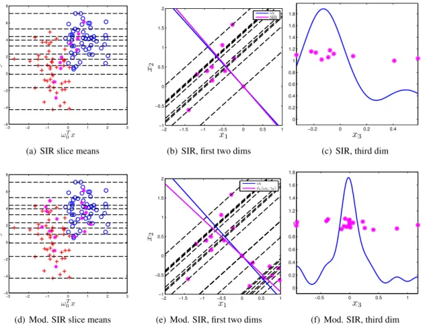
2.5.4 Illustrative Example
The modified SIR procedure described in the previous section is very similar to the original SIR procedure. The main difference is that the subgroup structure is taken into account in the former. Note that in SIR all termsX˜iX˜j0 are included in the covariance matrix whereas in the modification
only terms whereXi andXj lie on the same side of they hyperplaneωTX−γ = 0are included.
This additional restriction helps reduce the noise that can arise from aggregating across subgroups. To illustrate the noise issue, the performance of SIR is examined by studying a simple toy example. Set the parameters in Model (2.1) to the following:
n= 100, d= 3, ω0 = (
1 √
2,− 1 √
2,0), γ0 = 1 4, (µ1,0, σ21,0) = (0,4), (µ2,0, σ22,0) = (4,1),
−3 −2 −1 0 1 2 3 −6 −4 −2 0 2 4 6 8 ωT 0x y
(a) SIR slice means
−2 −1.5 −1 −0.5 0 0.5 1
−1 −0.5 0 0.5 1 1.5 2 x1 x2 ω0 SIR
(b) SIR, first two dims
−0.2 0 0.2 0.4 0 0.2 0.4 0.6 0.8 1 1.2 1.4 1.6 1.8 x3
(c) SIR, third dim
−3 −2 −1 0 1 2 3
−6 −4 −2 0 2 4 6 8 ωT 0x y
(d) Mod. SIR slice means
−2 −1.5 −1 −0.5 0 0.5 1
−1 −0.5 0 0.5 1 1.5 2 x1 x2 ω0 ˆ
νn(ω0, γ0)
(e) Mod. SIR, first two dims
−0.5 0 0.5 1
0 0.2 0.4 0.6 0.8 1 1.2 1.4 1.6 1.8 x3
(f) Mod. SIR, third dim
Figure 2.1: Toy example illustrating the differences between SIR and the proposed method of incorporating the surrogate variable described in Section 3.2.3. The estimateνˆn(ω0, γ0) is less
accurate than the SIR estimate in the first two dimensions but a better overall estimate across all three dimensions.
Note that the third component ofω0is 0 and thus the third dimension contains no information on the
subgroup structure. Despite the overlap between the distributionsN(0,4)andN(4,1), the surrogate variable clearly has valuable information for guiding classification.
The number of slicesH is set ton/10in both the modified and original SIR procedure. The top row in Figure 2.1 examines various aspects of the original SIR estimator for this toy dataset. Figure 2.1(a) plots the projection ofxonto the true directionω0against the surrogate variabley. The
circle and plus symbols correspond to the true subgroup membership. The asterisks in Figure 2.1(a) represent the sample meansmˆhwithin each slice whose boundaries are delineated by the horizontal
dashed lines. The slice means exhibit variation along theω0 direction moving across the slices.
Figure 2.1(b) shows the positions of the sample meansmˆh in the first two coordinates. The SIR
is 0.0545. Figure 2.1(c) shows the distribution of the slice means in the third coordinate. The slice means are not centered at zero despiteω0being zero in the third coordinate. This suggests the SIR
estimate will be inaccurate in the third coordinate. Indeed, the distance between the SIR estimate and ω0in the third coordinate is 0.2718, much higher than in the first two coordinates combined. Thus
although SIR is accurate in the first two coordinates, it is inaccurate in the third coordinate.
Next the performance of the modified SIR procedure on this toy example is examined. The second row in Figure 2.1 is as in the top row except the asterisks now represent the sample means
ˆ
mh,1(ω0, γ0)andmˆh,2(ω0, γ0)forh= 1, . . . , H. The distance betweenνˆn(ω0, γ0)andω0is 0.0888
in the first two coordinates, which is larger than the distance between the SIR estimate andω0.
However the accuracy in the third coordinate is a significant improvement over SIR. Figure 2.1(f) shows that the slice meansmˆh,1(ω0, γ0)andmˆh,2(ω0, γ0)in the third coordinate are centered at zero.
The distance betweenνˆn(ω0, γ0)andω0in the third coordinate is found to be 0.11. Thus, overall
across all three dimensions,νˆn(ω0, γ0)is more accurate than the SIR estimate.
2.6 Consistency
In this section, M-estimation theory is used to establish the consistency of the data-driven sieved maximum likelihood estimator(ˆωs
n,ˆγns). LetP denote the probability measure ofZ = (X, Y)under
Model 2.1. Define the empirical measure to bePn =n−1Pni=1δZi whereδz is the measure that
assigns mass 1 atzand zero elsewhere. For a measurable functionf, letPnf =n−1Pni=1f(Zi)be
the expectation off under the measurePnandP f = R
f dP the expectation underP. Using the empirical processes notation described above, the likelihood expression in Equation (2.2) can be rewritten as
Mn(ω, γ, θ(ω, γ)) =Pnmω,γ,θ(ω,γ)
where
mω,γ,θ(ω,γ)(x, y) =−log(σ2(x, ω, γ))−(y−µ(x, ω, γ))
2
σ2(x, ω, γ) . (2.9)
Note that the constant 1/2 and the log 2π terms have been dropped as they do not affect the maximization. The following assumptions are needed:
(A2) The univariate random variableωT
0Xhas a strictly bounded and positive densityfover[a, b]
withP(ωT
0X < a)>0andP(ω0TX > b)>0.
(A3) µ1,0=µ2,0andσ21,0 =σ22,0are not simultaneously true.
(A4) The surrogate variableY has finite first and second moments, i.e.EY <∞andEY2 <∞. (A5) For anyb∈Rp, the conditional expectationE(bX|ωT
0X)is linear inω0TX.
(A6) The covariateXhas a continuous distribution.
The interval[a, b]in (A1) may be estimated from the data by first calculating the direction of maximal variation of the sample covariatesX, and next considering the range of the resulting projections. The second assumption is satisfied for most continuous distributions ofXwhose support includes[a, b]. The third assumption ensures that the Gaussian mixture parameters are well defined. Assumption A4 is reasonable for most surrogate variables in practice. A5 is a key assumption in Li (1991) and is satisfied when the distribution ofXis Gaussian or more generally, elliptically symmetric. Finally Assumption A6 is necessary to guarantee the semi-continuity of the functionM(ω, γ, θ(ω, γ). Certain of these assumptions are for mathematical convenience and may be stronger than necessary. For instance the last assumption requiring the covariateXto have a continuous distribution is quite stringent and may be relaxed at the cost of more complicated proofs. The proposed method is later applied to real datasets in Section 2.9 that contain categorical covariates and the method is seen to perform well despite this.
Theorem 1. Let(X1, Y1), . . . ,(Xn, Yn)be iid from Model(2.1). Under (A1)-(A6), the data-driven
sieved maximum likelihood estimator defined in(3.5)using the boosted sieve in(3.8)is consistent for the true parameters(ω0, γ0).
Proof of Theorem 1. Following Theorem 14.1 (Argmax Theorem) in Kosorok (2008), the following will be established to show consistency: 1) The sequence(ˆωs
n,ˆγns)is uniformly tight; 2) The map
(ω, γ)7→M(ω, γ, θ(ω, γ))is upper semicontinuous with a unique maximum at(ω0, γ0); 3) Uniform
convergence ofMntoMover compact subsetsKofSp×[a, b], i.e.
sup
(ω,γ)∈K
in probability; and 4) The estimator “nearly” maximizes the objective function, i.e. ωˆs
n andγˆsn
satisfies
Mn(ˆωsn,ˆγns, θ(ˆωns,γˆns))≥Mn(ω0, γ0, θ(ω0, γ0))−oP(1).
The first condition is easily seen to hold. Since ωˆs
n is a unit vector in Rp, it is easy to see
||ˆωs
n||=OP(1). The intercept estimateγˆnslies in the interval[a, b]and is thus uniformly tight.
To check semi-continuity ofM(ω, γ, θ(ω, γ)), the conditional expectation ofmω,γ,θ(ω,γ)given Xis first examined. Taking the expectation with respect to the randomness inY gives
P(mω,γ,θ(ω,γ)(X, Y)|X)
=−log(σ2(X, ω, γ))−P{(Y −µ(X, ω, γ))
2|X}
σ2(X, ω, γ)
=−log(σ2(X, ω, γ))−P{(Y −µ(X, ω, γ))
21{ωTX−γ ≥0}|X}
σ2(X, ω, γ)
−P{(Y −µ(X, ω, γ))
21{ωTX−γ <0}|X}
σ2(X, ω, γ)
=−log(σ2(X, ω, γ))−P{(Y −µ1(ω, γ))
21{ωTX−γ ≥0}|X}
σ2(X, ω, γ)
−P{(Y −µ2(ω, γ))
21{ωTX−γ <0}|X}
σ2(X, ω, γ)
=−log(σ2(X, ω, γ))−P{(Y −µ1,0+µ1,0−µ1(ω, γ))
21{ωTX−γ ≥0}|X}
σ2(X, ω, γ)
−P{(Y −µ2,0+µ2,0−µ2(ω, γ))
21{ωTX−γ <0}|X}
σ2(X, ω, γ)
=−log(σ2(X, ω, γ))−[σ
2
1,0+ (µ1,0−µ1(ω, γ))2]1{ωTX−γ ≥0}
σ2(X, ω, γ)
−[σ
2
2,0+ (µ2,0−µ2(ω, γ))2]1{ωTX−γ <0}
σ2(X, ω, γ)
Taking expectation on both sides (this time with respect to the randomness inX) gives
M(ω, γ, θ(ω, γ)) =−log(σ21(ω, γ))P1{ωTX−γ ≥0} −log(σ22(ω, γ))P1{ωTX−γ <0}
− [σ
2
1,0+ (µ1,0−µ1(ω, γ))2]P1{ωTX−γ ≥0}
σ12(ω, γ)P1{ωTX−γ ≥0}+σ2
2(ω, γ)P1{ωTX−γ <0}
− [σ
2
2,0+ (µ2,0−µ2(ω, γ))2]P1{ωTX−γ <0}
σ2
1(ω, γ)P1{ωTX−γ ≥0}+σ22(ω, γ)P1{ωTX−γ <0}
SinceP1{ωTX−γ ≤0}is nonzero for(ω, γ)∈
Sp×[a, b], bothµ1(ω, γ)andσ12(ω, γ)are well
defined. Next, sinceX has a continuous distribution by Assumption A6, derivations in Lemma 2 in Appendix A showµ1(ω, γ) andσ12(ω, γ)are both continuous in (ω, γ). It can be similarly
shown µ2(ω, γ)and σ22(ω, γ) are continuous and well defined. Thus M(ω, γ, θ(ω, γ)) is upper
semi-continuous (in fact continuous) in(ω, γ).
Next the unique maximality of(ω0, γ0)is established. The conditional expectation of (Y −
µ(X, ω, γ))2givenXis uniquely minimized whenµ(X, ω, γ) =E(Y|X), i.e. whenω =ω 0and
γ =γ0. ThusM(·)is uniquely maximized at(ω0, γ0).
Establishing the third condition reduces to showing the individual classes of functions that comprise{mω,γ,θ(ω,γ)}are Glivenko-Cantelli with integrable envelopes. Next the fact that sums, differences, products, and compositions of GC classes with integrable envelopes are GC can be used. Lemma 2 in Appendix A provides the proof for this.
Finally the last condition of near maximization is checked. Lemma 3 in Appendix A establishes the existence of a sequenceωs
n∈Ωˆnthat converges toω0 and a corresponding sequence of intercept
estimatesγs
n∈[a, b]that converges toγ0. By definition, the sieve estimator(ˆωns,γˆns)satisfies
Mn(ˆωsn,ˆγns,θˆn(ˆωns,γˆns))≥Mn(ωsn, γns,θˆn(ωns, γns)). (2.10)
Lemma 4 in Appendix A shows that
|Mn(ωn, γn,θˆn(ω, γ))−Mn(ωn, γn, θ(ω, γ))| →0
in probability for any sequence(ωn, γn)∈Sp×[a, b]. Rewriting Equation (2.10) (by adding and
subtracting the same expressions) gives
0≤Mn(ˆωns,ˆγns,θˆn(ˆωsn,γˆns))−Mn(ˆωsn,ˆγns, θ(ˆωns,γˆns))
+Mn(ωns, γns, θ(ωsn, γns))−Mn(ωns, γns,θˆn(ωsn, γns))
Applying Lemma 4 to the second and third line above gives
Mn(ˆωns,ˆγns, θ(ˆωsn,γˆns))≥Mn(ωsn, γns, θ(ωns, γns))−oP(1). (2.11)
Now consider the following decomposition
|Mn(ω0, γ0, θ(ω0, γ0))−Mn(ωsn, γns, θ(ωns, γns))|
≤ |Mn(ω0, γ0, θ(ω0, γ0))−M(ω0, γ0, θ(ω0, γ0))|
+|Mn(ωns, γsn, θ(ωns, γns))−M(ωsn, γns, θ(ωns, γns))|
+|M(ωsn, γns, θ(ωns, γns))−M(ω0, γ0, θ(ω0, γ0))|.
The first two lines go to zero in probability by Lemma 2. The third line goes to zero in probability sinceMis continuous in(ω, γ)and(ωs
n, γns)converges to(ω0, γ0). Thus,
|Mn(ω0, γ0, θ(ω0, γ0))−Mn(ωns, γns, θ(ωsn, γns))| →0. (2.12)
in probability. Combining Equations (2.11) and (2.12) gives
Mn(ˆωns,ˆγns, θ(ˆωsn,γˆns))≥Mn(ωsn, γns, θ(ωns, γsn))−oP(1)
=Mn(ω0, γ0, θ(ω0, γ0))
−[Mn(ω0, γ0, θ(ω0, γ0))−Mn(ωsn, γns, θ(ωsn, γns))]−oP(1)
=Mn(ω0, γ0, θ(ω0, γ0))−oP(1).
Thus the near-maximization criterion for(ˆωs
n,ˆγns)is satisfied.
2.7 Model checking
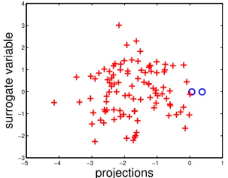
considered a less serious offense than splitting the sample into two subgroups when there is in fact no subgroup structure at all. It should be noted additionally the existence of numerous methods for determining the number of components in a finite mixture model. For instance it is common to add a penalty function, say based on the Bayesian inference criterion, to the main log likelihood term.
−5 −4 −3 −2 −1 0 1
−3 −2 −1 0 1 2 3 4
projections
surrogate variable
Figure 2.2: Estimated subgroups when there is actually only one component in the model. The plot here shows that the method gives a reasonable answer when there is only one component.
To understand what happens if the proposed method is applied to the setting where there is no subgroups structure at all, consider the following simulation setting. Letµ1,0 =µ2,0 = 0and
σ1,02 =σ22,0 = 1in Model (2.1). Let the dimension and sample size be set top= 5andn= 100, respectively. The covariateXis drawn from the standardp-variate Gaussian distribution. The first p/2components ofω0 are set to−p1/2and the rest top1/2, and the intercept is set to1/4. Figure
2.2 displays the projections onto the sieve estimated directionωˆs
nshifted by the estimated intercept
ˆ γs
nagainst the surrogate variabley. The resulting subgroups are indicated by different symbols and
are seen to be highly unbalanced as the plus subgroup contains merely two members. This greatly suggests that there is indeed only one component in the model.
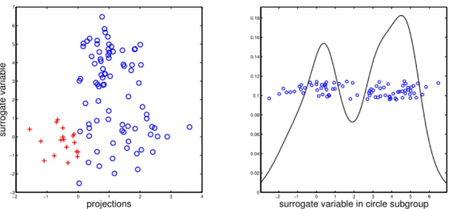
Another major violation of Model (2.1) occurs if the separating decision boundary is not linear inx. For concreteness consider the simulation setup above save for two changes – 1) the means and variances are set to(µ1,0, σ21,0) = (0,1)and(µ1,0, σ1,02 ) = (4,1)and 2) subgroup membership
−2 −1 0 1 2 3 4 −3
−2 −1 0 1 2 3 4 5 6 7
projections
surrogate variable
−2 −1 0 1 2 3 4 5 6
0 0.02 0.04 0.06 0.08 0.1 0.12 0.14 0.16 0.18
surrogate variable in circle subgroup
Figure 2.3: Left panel shows estimated subgroups when the decision boundary is not linear but quadratic. Right panel shows the bimodality of the surrogate variable in the circle subgroup. These plots suggest an easy visual tool to diagnose this type of assumption violation.
clearly bimodal. In general, if the two-component Gaussian mixture assumption is confirmed to hold, then this type of diagnostic suggests the boundary is not linear inx.
The two issues discussed above are major departures from Model (2.1). There are certainly other ways in which the presumed model may not hold – take departures from the normal distribution, for instance. This turns out to be a rather minor issue. For one, there exists many methods to transform a univariate random variable to have an approximate Gaussian distribution. Also, simulations in the next section suggest that the methodology is robust against non-Gaussianity of the surrogate variable.
There is also the question of how to assess whether the surrogate variable approximates well the underlying class label. This is an important, albeit philosophical, issue. In some cases, the selection of an appropriate surrogate variable can be guided by previous studies. When this is not possible, a surrogate variable can be chosen that is interesting in its own right. The binary outcome of interest can be defineda posterioriwith respect to the chosen surrogate variable. For instance, the surrogate variable “cholesterol level” is of interest in and of itself. The corresponding binary outcome of interest can then be defined with respect to this choice.
2.8 Simulations
noise to signal ratio is high. Lastly, a setting where the surrogate variable arises from the exponential distribution is considered. This is of interest because many outcome variables related to time can be well approximated by the exponential distribution. Since Model (2.1) assumes normality for the surrogate variable, this setting also tests how robust the methodology is to distributional violations in Model (2.1).
Simulation Setting Subgroup 1 Subgroup 2 Stochastically Ordered (SO) N(0,1) N(4,1) Non-stochastically Ordered (NSO) N(0,4) N(4,1) Variance Only (VO) N(0,1) N(0,4)
Exponentials (EXP) exp(1) exp(10)
Table 2.1: Description of simulation settings. The subgroups are determined by a hyperplane ωTX−γ= 0and the distributions of the surrogate variableY in each subgroup is given.
The vector of covariatesXis distributed as a standard multivariate Gaussian. Two different settings for the directionω0are considered. In the first setting, which shall be referred to as “sparse”,
all components ofω0 are set to zero except the first two which are set to(2−1/2,−2−1/2). This
reflects situations where only a few covariates matter. In the other setting, which shall be referred to as “abundant”, the firstp/2components ofω0are set to−p1/2and the rest top1/2. This reflects
situations where all the covariates drive the separation between the two subgroups. The intercept is set toγ0= 1/4which results in roughly60/40split of the data into two subgroups.
Different ratios of sample size to dimension are considered for the simulations. In the low dimensional problem the sample size is set ton= 100and dimension top= 5, andn= 200, p= 25 for the high dimensional. For the sparse setting, Tables 2.2 and 2.3 show the average norm difference between the estimate and the trueω0over 1000 Monte Carlo simulations for various settings. The
lowest average norm difference is highlighted in italics. The Tables 2.4 and 2.5 give the corresponding results for the abundant setting.
Settings NSO SO VO EXP Y Clustering 0.31 (0.11) 0.25 (0.09) 0.85 (0.31) 0.48 (0.18) X-Y Clustering 0.31 (0.11) 0.25 (0.08) 0.84 (0.33) 0.48 (0.18) EM 0.32 (0.15) 0.27 (0.13) 0.53 (0.23) 0.33 (0.13) Regression 0.25 (0.10) 0.19 (0.07) 1.07 (0.26) 0.36 (0.13) SIR 0.24 (0.09) 0.19 (0.07) 0.49 (0.23) 0.29 (0.12) Simple Sieve 0.22 (0.09) 0.20 (0.08) 0.33 (0.18) 0.24 (0.11) Proposed Method 0.14(0.07) 0.11(0.05) 0.30(0.16) 0.20(0.10)
Table 2.2: Sparse ω0, low dimensional setting. Average norm difference between estimate and
ω0 over 1000 Monte Carlo simulations. The standard error is given in the parentheses. The best
estimator (lowest norm difference) is highlighted in italics.
Settings NSO SO VO EXP
Y Clustering 0.52 (0.08) 0.43 (0.06) 1.13 (0.19) 0.75 (0.11) X-Y Clustering 0.52 (0.08) 0.43 (0.06) 1.14 (0.20) 0.75 (0.11) EM 0.50 (0.10) 0.43 (0.08) 0.78 (0.18) 0.54 (0.09) Regression 0.45 (0.07) 0.35 (0.06) 1.28 (0.10) 0.61 (0.09) SIR 0.44 (0.08) 0.34 (0.05) 0.82 (0.19) 0.54 (0.11) Simple Sieve 0.95 (0.11) 0.91 (0.11) 1.01 (0.13) 0.98 (0.12) Our Method 0.40(0.08) 0.31(0.05) 0.72(0.14) 0.49(0.10)
Table 2.3: Sparse ω0, high dimensional setting. Average norm difference between estimate and
ω0 over 1000 Monte Carlo simulations. The standard error is given in the parentheses. The best
estimator (lowest norm difference) is highlighted in italics.
especially high-dimensional settings. The best competitor appears to be the SIR method though the proposed method outperform it in every setting considered here, by large margins at times (see for instance the low-dimensional settings). Linear regression performs poorly in the low dimensional, VO setting. The simple sieve method is consistently among the worst in the high dimensional settings. The two clustering methods perform very similarly to each other and are decent for the NSO and SO settings, though they perform poorly for the VO and Exp simulations.
Settings NSO SO VO EXP Y Clustering 0.32 (0.12) 0.25 (0.09) 0.85 (0.33) 0.47 (0.17) X-Y Clustering 0.32 (0.12) 0.25 (0.09) 0.84 (0.34) 0.47 (0.17) EM 0.32 (0.15) 0.26 (0.12) 0.55 (0.23) 0.33 (0.13) Regression 0.25 (0.10) 0.20 (0.07) 1.05 (0.26) 0.36 (0.13) SIR 0.24 (0.09) 0.19 (0.07) 0.50 (0.24) 0.29 (0.12) Simple Sieve 0.22 (0.09) 0.21 (0.08) 0.35 (0.18) 0.25 (0.11) Proposed Method 0.14(0.07) 0.11(0.06) 0.33(0.18) 0.19(0.10)
Table 2.4: Abundantω0, low dimensional setting. Average norm difference between estimate and
ω0 over 1000 Monte Carlo simulations. The standard error is given in the parentheses. The best
estimator (lowest norm difference) is highlighted in italics.
Settings NSO SO VO EXP
Y Clustering 0.52 (0.08) 0.43 (0.06) 1.14 (0.19) 0.75 (0.11) X-Y Clustering 0.52 (0.08) 0.43 (0.06) 1.15 (0.19) 0.75 (0.11) EM 0.50 (0.09) 0.43 (0.07) 0.78 (0.18) 0.54 (0.08) Regression 0.45 (0.07) 0.35 (0.06) 1.28 (0.10) 0.61 (0.09) SIR 0.44 (0.08) 0.34 (0.06) 0.83 (0.19) 0.53 (0.10) Simple Sieve 0.94 (0.12) 0.90 (0.10) 1.01 (0.13) 0.98 (0.12) Proposed Method 0.41(0.08) 0.31(0.06) 0.72(0.13) 0.50(0.09)
Table 2.5: Abundantω0, high dimensional setting. Average norm difference between estimate and
ω0 over 1000 Monte Carlo simulations. The standard error is given in the parentheses. The best
estimator (lowest norm difference) is highlighted in italics.
2.9 Examples
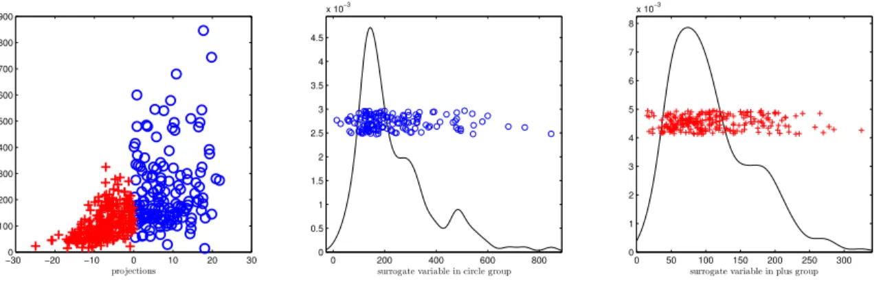
2.9.1 Pima Indian Diabetes Dataset
The Pima Indian Diabetes dataset contains information on 8 clinical measurements, including a 2-hour insulation measurement, for 768 individuals. It also records whether each individual later developed diabetes. The proposed method will be applied to find a diabetes and non-diabetes sub-group. The corresponding surrogate variable should approximately satisfy the normality assumption in Model (2.1) and be relevant to the binary event of interest. The 2-hour insulin measurement is a reasonable surrogate for the unobserved binary outcome and was approximately Gaussian. Furthermore, 374 out of the 768 total cases were missing the 2-hour insulin measurement. Since classification in the proposed method is completely determined by a separating hyperplane in the covariate space, it does not make use of the surrogate variable for classification of future objects. Thus the surrogate variable can be a quantity that is difficult to measure or obtain, as is the case here, since it is used only in the learning process.
−30 −20 −10 0 10 20 30
0 100 200 300 400 500 600 700 800 900 projections se ru m in su li n
0 200 400 600 800
0 0.5 1 1.5 2 2.5 3 3.5 4 4.5
x 10−3
surrogate variable in circle group
0 50 100 150 200 250 300
0 1 2 3 4 5 6 7 8
x 10−3
surrogate variable in plus group
Figure 2.4: Diabetes dataset. First panel shows the projections onto the estimated separating hyperplane versus the surrogate variable, 2-hour insulin. The second and third panels show the distribution of the surrogate variable in each of the discovered subgroups.
The projections of the covariates onto the estimated separating hyperplane is shown in the first panel of Figure 2.4. A smoothed histogram of the 2-hour insulin measurement in each discovered subgroup is shown in the next two panels of Figure 2.4. There is a bit of departure from Gaussianity here but it does not seem severe enough to affect the performance of the method. The circle subgroup corresponds well with the individuals who later develop diabetes and the plus subgroup with those who did not.
the misclassification rate on this test set. The error rates of logistic regression and three “off-the-shelf” methods described in Section 2.4 – Y Clustering, X-Y clustering, and the EM algorithm – are also examined. The bottom row in Table 2.6 shows the performance of each method for this data example. To make the methods comparable, the surrogate variable used in the proposed method is not included in the logistic regression model. Logistic regression is a rather minor improvement over the proposed method considering it requires trained labels. The EM, Y clustering, and X-Y clustering are all slightly less accurate than the proposed method.
Dataset the proposed method Logistic Regression Y Clustering X-Y Clustering EM Heart 0.23 (0.06) 0.18 (0.04) 0.40 (0.05) 0.43 (0.09) 0.41 (0.05)
Diabetes 0.27 0.26 0.29 0.29 0.30
Table 2.6: Classification accuracy. For the Heart dataset, accuracy is measured by 10-fold cross validation. Standard error across the folds is given in the parentheses. For the Diabetes dataset, accuracy is measured by the test error on a held-out test set of 374 cases who are missing the 2-hour insulin measurement.
2.9.2 Cleveland Heart Disease Dataset
This dataset contains information on heart disease for 297 individuals. There are 13 clinical measurements in addition to the diagnosis, i.e. presence/absence of heart disease. The data was collected from the Cleveland Clinic Foundation. The proposed method was applied to find a subgroup with heart disease and a subgroup without. The maximum-heart-rate-achieved variable was chosen as the surrogate variable because it was approximately normally distributed and is correlated to cardiac mortality (MS et al., 1999).
The projections of the covariates onto the estimated separating hyperplane is shown in the first panel of Figure 2.5. A smoothed histogram of the maximum-heart-rate measurement for each discovered subgroup is shown in the last two panels of Figure 2.5. The Gaussian assumption seems to hold quite well and there is no indication that the two component structure is incorrect. The plus subgroup corresponds well with the individuals who were diagnosed with heart disease and the circle subgroup with those who were not.
−3 −2 −1 0 1 2 3 60 80 100 120 140 160 180 200 220 projections m a x im u m -h ea rt -r a te -a ch ie ve d
100 120 140 160 180 200
0 0.005 0.01 0.015 0.02 0.025
surrogate variable in circle subgroup
80 100 120 140 160
0 0.002 0.004 0.006 0.008 0.01 0.012 0.014 0.016 0.018 0.02
surrogate variable in plus subgroup
Figure 2.5: Heart dataset. First panel shows the projections onto the estimated separating hyperplane versus the surrogate variable, maximum-heart-rate achieved. The second and third panels show the distribution of the surrogate variable in each of the discovered subgroups.
relatively well considering it does not use labeled data at all. The other methods, EM, Y clustering, and X-Y clustering, perform quite poorly for this dataset.
2.9.3 Prostate Cancer Dataset
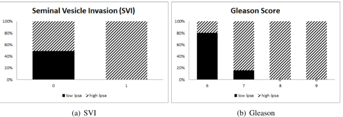
The Prostate dataset comes from a study which examined the relationship between the level of PSA and certain clinical measures in men who were about to receive a radical prostatectomy. The dataset has information on 97 subjects and 8 covariate measurements. Using the log PSA (lpsa) as the surrogate variable, the proposed method is applied to find two subgroups that differ in terms of log PSA. There is no binary outcome variable provided in this dataset. However, PSA is known to be associated with more severe grades of prostate cancer so the binary outcome could be taken to be “more severe” versus “less severe” grades of prostate cancer.
Figure 2.6 is a scatterplot of the continuous covariates in the Prostate dataset. The subgroups found by the proposed method are displayed as different symbols, with the circle subgroup having higher log PSA. Taking a look at Figure 2.6, patients with higher log PSA (circle) indeed have higher log cancer volume (lcavol) and log prostate weight (lweight).
−2 0 2 0
0.2
lcavol
−1 0 1
0 0.5
lweight
−1 0 1 2
0 1 2
lbph
−1 0 1 2 3
0 1 2
lcp
−1 0 1
−2 0 2 lweight lc av o l
−1 0 1 2
−2 0 2 lbph lc av o l
−1 0 1 2 3
−2 0 2 lcp lc av o l
−2 0 2
−1 0 1 lcavol lw ei g h t
−1 0 1 2
−1 0 1 lbph lw ei g h t
−1 0 1 2 3
−1 0 1 lcp lw ei g h t
−2 0 2
−1 0 1 2 lcavol lb p h
−1 0 1
−1 0 1 2 lweight lb p h
−1 0 1 2 3
−1 0 1 2 lcp lb p h
−2 0 2
−1 0 1 2 3 lcavol lc p
−1 0 1
−1 0 1 2 3 lweight lc p
−1 0 1 2
−1 0 1 2 3 lbph lc p
Figure 2.6: Scatterplot of the continuous covariates in the Prostate dataset. A complete list of the full names of the variables is given in Appendix A. The symbols represent the subgroups found by the proposed method where the circle subgroup has higher lpsa values on average. Note that the circle group has higher log cancer volume (lcavol) and higher log prostate weight (lweight), two variables that are linked to the severity of the cancer.
2.10 Discussion
(a) SVI (b) Gleason
CHAPTER 3: LATENT SUPERVISED LEARNING FOR SURVIVAL DATA 3.1 Introduction
Latent supervised learning is a machine learning technique for performing binary classification using a surrogate variable when labeled training data is unavailable. Wei and Kosorok (2013) first introduced this idea and applied it to a model wherein the surrogate variable is Gaussian distributed. Here we extend the methodology to the surrogate variable that is a right-censored survival time.
The proposed methodology is particularly motivated by the problem of stratifying a population into two risk groups based on a set of biomarkers. One rather naive approach for risk stratification is to cluster the patients based solely on biomarkers. This approach ensures patients with similar biomarker values are assigned to the same subgroup. There is no guarantee, however, that the resulting clusters will exhibit different survival experiences. Another approach is to stratify patients based solely on survival time. This, however, is likely to have the undesirable effect of producing subgroups of patients in the same risk group with dissimilar biomarker patterns.
The proposed methodology can be applied to discover subgroups that are both biologically and clinically meaningful. An index using the the binary rule ”index<cutpoint” is constructed to divide the population into two subgroups. The index is chosen to be a linear combination of the biomarkers to be estimated from the data. Our model takes the classic Cox model as a starting point. LetT denote the true (unobservable) lifetime andC the censoring time. The observed data consists of Y = min(T, C),δ = 1{T ≤C}and a realp-dimensional covariate vectorX. The proposed model assumes the linear hyperplane in the covariate space defined byωT
0x−γ0 = 0, whereω0 ∈Rpand
γ0 ∈R, “separates” the survival times into two distributions with proportional hazards. Accordingly,
the conditional hazard function is given by
whereh0(t)is the baseline hazard function andβ0is the log hazards ratio, assumed to be nonzero for
identifiability. It is further assumed that censoringCis independent of survivalT, conditional onX. In the estimation of Model (3.1), the primary parameters of interest areω0andγ0. The estimation
procedure used in the Gaussian model in Wei and Kosorok (2013) will be adapted for Model (3.1) to account for censoring. The estimation is obtained by maximizing the Cox proportional hazards partial likelihood over a data-driven sieve, an approximating space constructed to grow dense as sample size increases.
3.1.1 Related work
Tian and Tibshirani (2011) proposed the adaptive index model which constructs a score that is the sum of several binary rules such as “age> 60” or “blood pressure> 120mm Hg”. The conditional hazard function in an adaptive index model is given by
h(t|x) = exp(β0+β K X
k=1
1{x∗k≤ck})h0(t), (3.2)
wherex∗kare from the set{±x1, . . . ,±xp}andK, the number of binary rules, is no bigger thanp,
the dimension of the covariate vectorX.
In both Model (3.1) and (3.2), the covariate space is divided into regions with different survival experiences. As linear boundaries offer an especially rich and flexible array of binary partitions in high dimensions, Model (3.1) may in this regard have certain advantages over the adaptive index model in which boundaries always remain parallel to the coordinate axes.There is also no need to pre-specify in the proposed model the number of covariates to include in the final stratification rule. This is to be contrasted with the requirement thatK in Model (3.2) be carefully chosen. Variable selection is built into the proposed methodology since all covariates are assigned a weight which give an indication of the importance of a variable.
data (Leblanc and Crowley, 1993; Banerjee and Noone, 2007). Another generalization is multivariate trees, see for instance Gama (2004), which allow for a linear combination of variables at decision and leaf nodes rather than a single variable.
Trees combine binary rules constructed using univariate variables. In contrast, the proposed methodology constructs a single binary split based on a linear combination of all variables. While tree-based methods allow for finer risk stratification, the proposed methodology can offer easier interpretation. For instance, patients that belong to neighboring nodes in a tree-based survival model may exhibit very different survival outcome even though their covariate patterns are similar. The richness of linear decision boundaries in high dimensions makes a further case for studying a parsimonious model as in Model (3.1). Also, there are fewer tuning parameters involved in the proposed methodology whereas in many tree-based methods, careful decisions have to be made regarding growing the tree and then pruning it back.
There are also several related works in the literature that deal with risk stratification using non-tree approaches. One such methodology was put forth in Bair and Tibshirani (2004). There, a continuous predictor of survival based on gene expression is constructed and a threshold on the predictor is used to identify two subgroups. The procedure has two steps: 1) a subset of genes with the highest Cox scores is selected, and 2) principal components analysis is performed on this subset of the gene expression data, and a proportional hazards model based on the first few principal components is used to obtain a continuous predictor of survival. A disadvantage of this two-step procedure is that genes which do not play a strong individual role but play an important role when considered in an ensemble of genes will be completely removed in the first step.
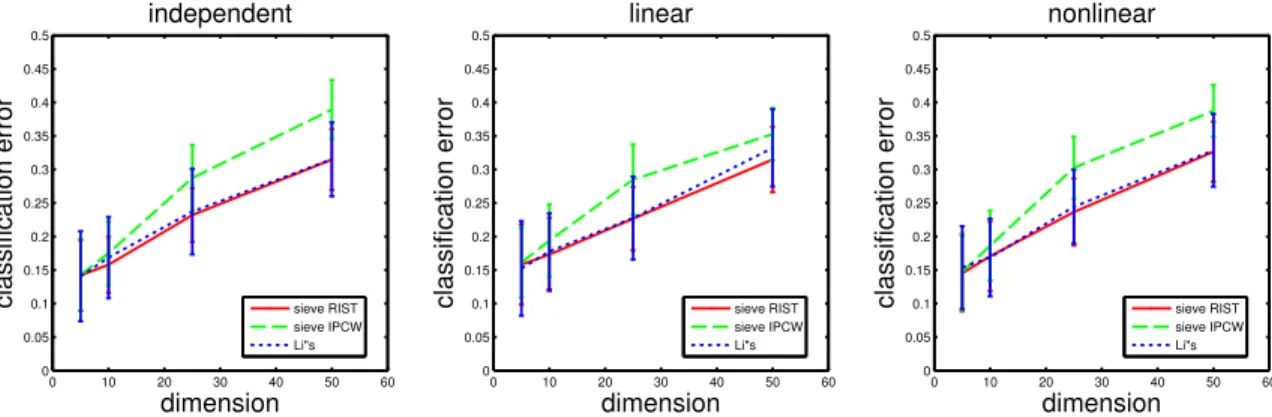
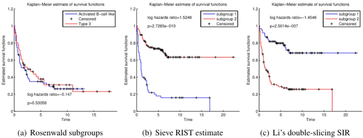
In the simulations and data examples found later in this chapter, we will directly compare the proposed methodology to a method proposed in Li et al. (1999), which will be referred to as Li’s double-slicing method. This method is based on the dimension reduction technique Sliced Inverse Regression (SIR) (Li, 1991). The SIR model assumes the response variableT ∈Ris related to the covariate vectorX ∈Rpin the following manner: