Bayesian density regression and predictor-dependent clustering

(1)

BAYESIAN DENSITY REGRESSION AND

PREDICTOR-DEPENDENT CLUSTERING

by Ju-Hyun Park

A dissertation submitted to the faculty of the University of North Carolina at Chapel Hill in partial fulfillment of the requirements for the degree of Doctor of Philosophy in the Department of Biostatistics, School of Public Health.

Chapel Hill 2008

Approved by:

(2)

(3)

ABSTRACT

JU-HYUN PARK: Bayesian Density Regression and Predictor-Dependent Clustering.

(Under the direction of Dr. David Dunson.)

Mixture models are widely used in many application areas, with finite mixtures of Gaus-sian distributions applied routinely in clustering and density estimation. With the increasing need for a flexible model for predictor-dependent clustering and conditional density estimation, mixture models are generalized to incorporate predictors with infinitely many components in the semiparametric Bayesian perspective. Much of the recent work in the nonparametric Bayes literature focuses on introducing predictor-dependence into the probability weights.

(4)

ACKNOWLEDGMENTS

This thesis is the end of the first act of a play entitled “Ju-Hyun, Professional Biostatistician.” I don’t think that it would have been possible for me to have finished the first act without help and support from many people.

First, I am very grateful to my thesis advisor, Dr. David Dunson. In addition to his insightful comments and advice, he gave me the encouragement and confidence to get through all the hardships that I encountered in my research. In Korea it is believed that a person has three major life-changing opportunities in his/her life. I believe that this was one of my three opportunities to have Dr. Dunson as my thesis advisor.

I thank Dr. Amy Herring who encouraged me to pursue to the Ph.D program in Biostatistics at UNC-CH. Whenever I was depressed or had troubles in my life, she was my personal counselor. Her warm words of wisdom and encouragement rescued me out of the swamp of emotional instability.

I thank my committee members, Dr. Michael Kosorok, Dr. Hongtu Zhu, and Dr. Kenneth Bollen, for their support. Their valuable comments made my thesis more fruitful. I also thank the faculty and staff in Biostatistics for their kind assistance and guidance.

I am grateful to the Collaborative Studies Coordinating Center, UNC-CH, and the Biostatis-tics Branch in the National Institute of Environmental Health Sciences for the experience and financial support they provided me.

Finally, I thank my entire extended family for their support. Although they live in Korea, I feel as though they are here beside me. Their warm words in emails and calls gave me strength to carry on my studies. I dedicate my thesis to my parents, Youngcho Park and Jungnim Shin.

(5)

LIST OF FIGURES

2.1 Results for the first simulation example . . . 30

2.2 Comparison of estimated densities between the PPM and the GPPM . . . 31

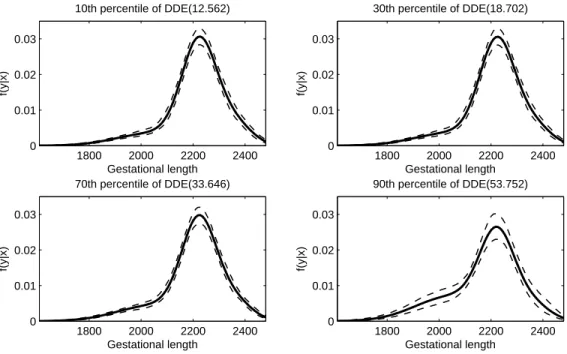
2.3 Estimated predictive densities for GAD at different DDE levels . . . 33

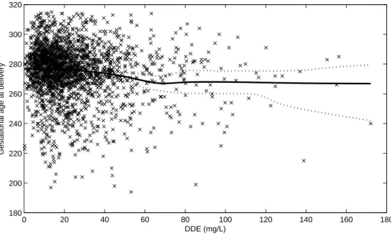
2.4 The conditional predictive mean of GAD . . . 34

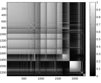
2.5 Pairwise marginal probabilities of being grouped with another subject in the CPP data. . . 35

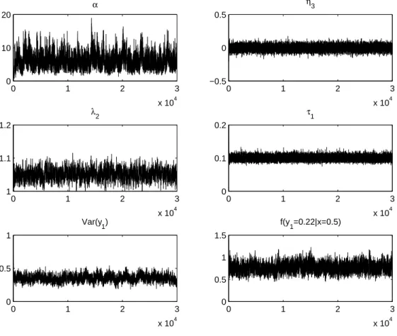
3.1 Trace plots of representative quantities. . . 51

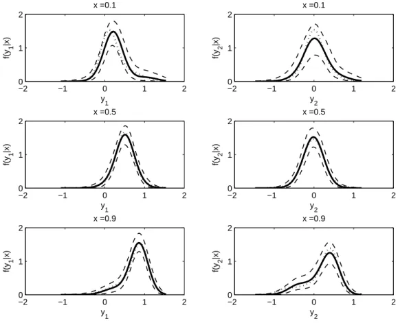
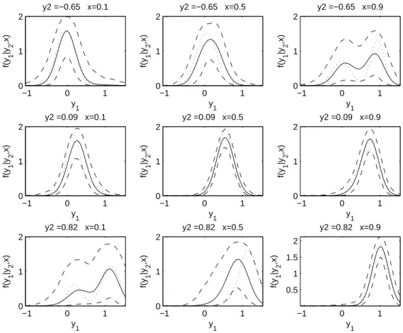
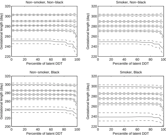
3.2 Estimated predictive conditional densities of y1 and y2 given xin simulation study 53 3.3 Estimated predictive conditional density of y1 given y2 and x in simulation study 54 3.4 Percentile plots of estimated conditional GAD density over percentiles of DDT by smoking status and ethnic group . . . 55

3.5 Percentile plots of estimated conditional BW density over percentiles of DDT by smoking status and ethnic group . . . 56

3.6 Heat plot of the marginal probability for a comparison of conditional densities by ethnic group . . . 58

3.7 Profile of estimated conditional densities of BW for different values of GAD . . . 59

4.1 Trace plots of representative quantities in simulation case 1. . . 71

4.2 Estimated conditional density of y given xin simulation case 1 . . . 72

4.3 Cross-validation results for prediction of y in simulation case 1 . . . 73

4.4 Estimated conditional density of y given xin simulation case 2 . . . 74

4.5 Cross-validation results for prediction of y in simulation case 2 . . . 75

(9)

LIST OF TABLES

(10)

CHAPTER 1 INTRODUCTION AND

LITERATURE REVIEW

1.1 Introduction

Mixture models are widely used in many application areas, with finite mixtures of Gaussian distributions applied routinely in clustering (Day, 1969; Binder, 1978; Symons, 1981) and density estimation (Roeder and Wasserman, 1997; Richardson and Green, 1997). A recent review of the use of mixture models in clustering and density estimation can be found in Fraley and Raftery (2002).

(11)

Motivated by such research problems and the successful use of mixture models characteriz-ing univariate and multivariate distributions, several attempts have been made to generalize the mixture models to incorporate predictors. A finite mixture of linear regressions has been the most widely used, with the probability weights assigned to components being either fixed (Viele and Tong, 2002) or modeled by a parametric regression model, commonly polytomous logistic regression. Hierarchical mixtures-of-experts models (Jordan and Jacob, 1994) in the machine learning literature instead use a probabilistic decision tree to model the probability weights. An alternative is a mixture of multivariate normals, which induces a conditional response distribu-tion given predictors as a locally weighted mixture of normal regression models, as in M¨uller et al. (1996).

There is a potential criticism on limited flexibility of a finite mixture of linear regression models due to its formulation. In finite mixture models, some a priori knowledge on the number of components is necessary and subjects are assigned to one of the preselected number of com-ponents. In this sense, the semiparametric Bayesian approach has been considered to provide a flexible mixture model that incorporates prior information but is free of the restriction on the number of components. From the Bayesian formulation, infinite mixture models can be obtained by assuming the mixture distribution to be generated from a stick-breaking prior, commonly the Dirichlet process (DP) (Ferguson, 1973; 1974) prior. With a remarkable advance in devel-oping Monte Carlo Markov chain (MCMC) methods, rich literature has been contributed to the Dirichlet process mixture (DPM) models (Lo, 1984; Escobar, 1994; Escobar and West, 1995).

Despite its flexibility in incorporating infinite number of linear regression models, a DPM of linear regressions itself is not appropriate for predictor-dependent clustering and conditional density estimation. Under the model, the probability weights are fixed and constant over the predictor space, implying that subjects are interchangeable and predictors are not informative about the clustering. The fixed probability weights also restrict a conditional response mean to be linear.

(12)

order-based dependent Dirichlet process, where the ordering of beta variates in the stick-breaking construction depends on predictors. As an alternative, Dunson et al. (2007) proposed a kernel-weighted mixture of DPs (WMDP), where the weights are proportional to the product of spatial closeness in the predictor space measured through a kernel and random weights assigned at the predictor values observed in the sample. Dunson and Park (2008) defined the kernel-stick breaking process (KSBP) by introducing independent random probability measures and beta-distributed random weights at each of infinite sequence of random locations. The probability weights are sequentially allocated by randomly breaking a probability stick (starting with a stick of length 1) and allocating the probability broken off to a basis location, with the length of each break being proportional to the product of a kernel and the assigned random weight. In addition, the latter two approaches have a desirable sparsity-favoring structure in which the introduction of additional mixture components is automatically penalized and the base parametric model is used to interpolate across sparse data regions.

Although the WMDP and KSBP are very flexible and can be implemented with a straightfor-ward Markov chain Monte Carlo (MCMC) algorithm, a potential criticism is expensive computa-tion in posterior sampling. There are many unknown parameters needed in defining such priors, including smoothing parameters in a kernel. The number of smoothing parameters increases as there are more predictors, resulting in the computational burden. In Dirichlet process mixture models, a common strategy to reduce expensive computation is to rely on a marginalized model that integrates out the infinitely-many parameters characterizing the process to induce a finite parameter sampling distribution through a random partition of subjects into clusters (Quintana and Iglesias, 2003; Quintana, 2006). A similar approach has yet to be developed that allows predictor-dependence in partitioning.

With a focus on the applications of predictor-dependent clustering and conditional density estimation, this dissertation proposes three semiparametric Bayesian methods, which greatly re-duce computational burden while facilitating simpler interpretations through the use of predictor-dependent partition models induced through marginalizing joint nonparametric process models. The first method focuses on generalizing the product partition model (Hartigan, 1990; Barry

(13)

and Hartigan, 1992) to incorporate predictors in its clustering process. The underlying idea is based on marginalizing out the parameters characterizing the predictor-component of the joint modeling approach of M¨uller et al. (1996). This allows us to obtain a generalized P´olya urn scheme, which incorporates predictor-dependent weights in a simple and intuitive manner. The development of this urn scheme is the main theoretical contribution of the thesis, with the re-mainder of the thesis focusing on using the result to obtain methods that allow latent variable distributions in hierarchical models to be unknown and predictor-dependent.

(14)

1.2 Literature Review

1.2.1 Nonparametric Bayes

In statistical modeling, one of the commonly-faced problems is how to model an unknown probability distribution for responsey. The easiest way to do this is to find a class of distributions in a parametric family, which usually provide us with ease of implementation and interpretation of a statistical model. In analyzing real data, however, it is quite common to have a belief that observed data don’t follow any known parametric distribution. This leads to modeling with an inadequate parametric assumption, often resulting in unreasonable inference. For this reason research interest has been taken to nonparametric methods as a way of getting very flexible models, typically defined by removing the parametric assumption.

Much of work on nonparametric inference has been achieved in the frequentist perspective. However, there are some attractive advantages of the Bayes formulation. First, it provides a full probabilistic characterization of the problem, which automatically allows for estimation uncertainty. It also provides a natural framework for inclusion of prior information allowing for shrinkage and centering on parametric models, limiting the curse of dimensionality. Finally, it allows embedding in larger hierarchical models, so that one can easily account for complicating features of the analysis, such as missing data, censoring, and model uncertainty. In this respect, nonparametric Bayesian inference is accomplished by defining probability models with infinite-dimensional parameters (Bernardo and Smith, 1994; M¨uller and Quintana, 2004). A collection of nonparametric Bayesian papers can be found in Ghosh and Ramamoorthi (2003). For a recent review on nonparametric inferences, refer to M¨uller and Quintana (2004).

1.2.2 Random Probability Measure

In the nonparametric Bayesian formulation, one can allow an unknown distribution by defin-ing a probability measure on a collection of distribution functions. More formally, a prior can be induced on a distribution by defining a random probability measure (RPM). According to

(15)

Ferguson (1973) and Antoniak (1974), there are two desirable properties of RPMs: (I) the prior distribution should have large support; (II) given a sample of observations, posterior distribution should be analytically manageable. In addition to the desirable properties mentioned in these earlier papers, there are a number of other properties considered in more recent work, such as posterior consistency (Ghosal et al., 1999; Lijoi et al., 2005; Walker et al., 2007) and existence of Bernstein von Mises theorems (Freedman, 1999).

1.2.2.1 Dirichlet Process

The Dirichlet process (DP) (Ferguson, 1973; 1974) has been most popular and playing a key role in the nonparametric Bayesian literature. Let Y be a space andA a σ-field of subsets, and letF0 be a finite non-null measure on (Y,A). Suppose thaty= (y1, . . . , yn) follow the following

model:

yi iid∼F, F ∼DP(αF0), (1.1)

where DP(αF0) denotes a DP with precision α and base measure F0. RPM F is said to follow a DP prior, DP(αF0), if for any measurable partition (A1, . . . , Ak) of Y, the vector of

(F(A1), . . . , F(Ak)) follows a Dirichlet distribution, D(αF0(A1), . . . , αF0(Ak)). For A∈ A, the

DPP has the following properties:

1) E(F(A)) =F0(A) and V(F(A)) = F0(A)(1−F0(A))/(1 +α)

2) F|y∼DP(α∗_F∗

0), where α∗ =α+n and F0∗ = (F0+

P_n

i=1δyi)

These properties imply that precision α controls the concentration on base measure F0 with a large value expressing confidence that F0 provides a good approximation, so that there is a high degree of shrinkage toward F0 in the posterior, which has a conjugate form being also a DP.

(16)

MacQueen (1973) P´olya urn scheme, obtained upon marginalizing over the prior over F:

P(y1 ∈ ·) = F0(·),

P(yi ∈ ·|y1, . . . , yi−1) =

µ

α α+i−1

¶

F0(·) +

i−1

X

j=1

µ

1

α+i−1

¶

δyj(·), (1.2)

it is obvious that the response yi for subject i either takes a value newly generated from

nonatomic base measure F0 with probability α/(α+i −1) or is set equal to one of the ex-isting values (y1, . . . , yi−1) chosen by sampling from a discrete uniform. This induced clustering process is also known as the CRP (Chinese Restaurant Process) (Aldous, 1985), the name of which originates from a sequential seating arrangement in a Chinese restaurant: customers sequentially enter a restaurant which have an infinite number of tables capable of having an unlimited number of customers, the first customer is seated at an empty table, and the ith cus-tomer can be seated either at a new table with probability α/(α+i−1) or at one of the tables occupied by the first i−1 customers with probability proportional to the number of customers seated at that table.

The DP can be alternatively constructed, based on Sethuraman’s (1994) stick-breaking rep-resentation. RPM F in expression (1.1) can be equivalently expressed as

F =

∞

X

h=1

πhδy∗

h, πh =Vh

h−1

Y

l=1

(1−Vl), Vh iid∼beta(1, α), y∗h iid

∼ F0. (1.3)

and from this expression, it follows that the DP is discrete with probability one.

1.2.2.2 Other RPMs

There have been many RPMs in the literature, which have a more general form than that of the DP, but we focus ourselves on a few most popular ones.

In expression (1.1), one can have a RPM associated with a species sampling model (SSM) (Pitman, 1996) by replacing the DPP with a random distribution, which has a functional form

(17)

as

F =

∞

X

h=1

whδy∗

h+

µ

1−

∞

X

h=1

wh

¶

F0, (1.4)

where atoms {y∗

h}∞h=1 are sampled from base measure F0 independent of weights {wh}∞h=1, with

P(P∞_h₌₁wh ≤1) = 1 andwh being interpreted as the relative frequency of thehth species with

tag equal to y∗

h in a certain large population of various species. If P(

P_∞

h=1wh = 1) = 1 and F0 is nonatomic, then the distribution in expression (1.4) is discrete. SSMs are flexible and rich, including finite-dimensional Dirichlet-multinomial process (Muliere and Secchi, 1995), the DP, its two-parameter extension, the two-parameters Poisson-Dirichlet process (Pitman and Yor, 1997), and the beta two-parameter process (Ishwaran and Zarepour, 2000) as special cases.

Another important class of RPMs is stick-breaking priors (Muliere and Tardella, 1998; Ish-waran and James, 2001), which can be also seen as a special case of expression (1.4). According to their definition, a stick-breaking prior has a form of

F =

N

X

h=1

whδy∗

h,

where for 1 ≤ N ≤ ∞, {y∗

h}Nh=1 are independent and identically distributed draws from F0, {wh}Nh=1 are probability weights with wh = Vh

Q

l<h(1−Vl), where Vh ind∼ Beta(ah, bh). Some

notable examples of stick-breaking priors are the two-parameters Poisson-Dirichlet process (with parametersah = 1−aandbh =b+ka), the beta two-parameter process (with parametersah =a

and bh =b), and the DP (with parameters ah = 1 and bh =α) for N → ∞.

The last, but not least, RPM we consider is the P´olya tree (PT) (Lavine, 1992; 1994), which is a generalization of the DP. The PT is defined by a set Π = {πl, l= 1,2, . . .}of nested binary

partitions of the sample space Y. The PT is initiated by splitting the spaceY into two disjoint subsets π1 ={B0, B1} and continues to partition the subsets, with the partition at levell being represented as πl = {B², ² = ²1. . . ²l}, where ² is a binary string of length l with ²j ∈ {0,1}.

(18)

nonnegative numbers C = {c²} and random variables Z = {Z²} with Z² ind∼ Beta(c²0, c²1) and for every l= 1,2, . . . and every²=²1. . . ²l,

F(B²1...²l) =

µ _Yl

j=1;²j=0

Z²1...²j−1

¶µ _Yl

j=1;²j=1

(1−Z²1...²j−1)

¶

.

The PT has the following properties: 1) Different from the other RPMs we considered in this subsection, continuous distributions can be generated from the PT with a certain choice of parameters, such as c²1...²l = l

2_{; 2) The PT is a conjugate prior,} _F_|_y _∼ _{P T}_(Π_,_C∗_{), where}

C∗ ₌_c

²+n² and n² is the number of observations inB² (Ferguson, 1974; Lavine, 1994) The DP

is a special case of the PT with c² =c²0+c²1.

1.2.3 Mixture models

1.2.3.1 Finite mixture models

Suppose that the response Yi follows one of k (usually <∞) group-specific densities fh(·) =

fh(θh), characterized by finite dimensional parameter θh ∈ Ψ (often Ψ = Rd) in a parametric

family, with probability ph, and then a (parametric) mixture model for Yi is defined as

p(yi) = k

X

h=1

phfh(yi|θh). (1.5)

By introducing an unobservable (latent) variableSi, withSi =hdenoting that subject ibelongs

to thehth mixture component, expression (1.5) can be equivalently expressed in hierarchial form as

Yi|Si ∼ f(θSi)

Si ∼ Multinomial({1, . . . , k};p), (1.6)

(19)

where p = (p1, . . . , pk), and thus S = (S1, . . . , Sn) completely determines a partition of n

subjects into k ≤n clusters. With respect to the interpretation of these models, the former can be viewed as a semiparametric construction as an alternative to nonparametric models, whereas the latter is the missing data formulation (Jasra et al., 2005). For a recent review of the use of finite mixture models in various applications, refer to Fraley and Raftery (2002).

In order to generalize (1.5) to incorporate predictors x= (x1, . . . , xp), one can model

predic-tor dependence in π = (π1, . . . , πk)0 and/or f(θh),h= 1, . . . , k, as follows:

f(y|x) =

k

X

h=1

πh(x)fh(y|θh,x).

For example, hierarchical mixtures-of-experts models (Jordan and Jacobs, 1994) character-ize πh(x) using a probabilistic decision tree, while letting f(y|θh) = N(y;x0βh, τh−1) with

θh = (β0h, τh)0 correspond to the conditional density for a normal linear model. The term

“ex-pert” corresponds to the choice of f(y|θh,x), as different experts in a field may have different

parametric models for the conditional distribution. A number of authors have considered alter-native choices of regression models for the weights and experts (e.g., Jiang and Tanner, 1999). For recent articles, refer to Carvalho and Tanner (2005), Ge and Jiang (2006), and Geweke and Keane (2007).

1.2.3.2 Mixture Models with RPMs

Due to the discrete feature of the RPMs in section 1.2.2, they are not suitable for use as a prior on continuous densities. To avoid this constraint, discrete RPMs are often used as a mixing distribution in the mixture model framework, and the model can be expressed in hierarchical form as

yi|φi ind∼ f(φi)

φi iid∼ G

(20)

often resulting in an infinite mixture model. For example, using Sethuraman’s (1994) stick-breaking representation of the DP in (1.3), the mixture model with a choice of G∼ DP(αG0) in expression (1.7), can be expressed as

p(yi) = ∞

X

h=1

πhfh(yi|θh), (1.8)

where πh and Vh are the same as in expression (1.3), but {θh}∞h=1 are an iid sample from base measure G0, and this model is often referred to as the Dirichlet process mixture (DPM) models (Lo, 1984; Escobar and West, 1995). For mixture models with other RPMs, refer to the following papers: Ishwaran and Jaems (2003) and Navarrete et al. (2008) (for the RPM associated with the SSM), Ishwaran and James (2001) (for the stick-breaking prior), and Hanson and Johnson (2002), Paddock et al. (2003), and Hanson (2006) (for the PT).

With a focuss on the DPM models, there have been rich contributions to developing algo-rithms for posterior computation, and most of algoalgo-rithms follows one of the three main ap-proaches: the marginal approach, the conditional approach, and the split-merge approach. In order to avoid the need for expensive computation for the infinite-dimensional G, the marginal approach is to marginalize over the Dirichlet process, resulting in the P´olya urn scheme (Black-well and MacQueen, 1973), which plays a key role in the Gibbs sampling methods (Escobar, 1994). Based on expression (1.2), the Gibbs sampling proceeds by sequentially sampling φi from

its full conditional distribution

(φi|φ(i),y, α) ∼ qi0Gi,0+

k(i)

X

h=1

qihδ_θ(i)

h , (1.9)

where θ(i) _{= (}_θ(i) 1 , . . . , θ

(i)

k(i)) is the k(i) unique values of φ(i) = (φ1, . . . , φi−1, φi+1, . . . , φn), the

posterior Gi,0(φ) is

Gi,0(φ) =

G0(φ)f(yi|φ)

R

f(yi|φ)dG0(φ)

= G0(φ)f(yi|φ)

hi(yi)

,

(21)

qi0 =c wi0hi(yi),qih=c wihf(yi|θh), and c is a normalizing constant. Due to a possibility of slow

mixing, Bush and MacEachern (1996) modified the Gibbs sampling algorithm by updating the cluster specific parametersθseparately from the cluster membership indicatorsS= (S1, . . . , Sn),

withSi =hifφi =θh. Jain and Neal (2004) mentioned that in a case where mixture components

are similar in terms of parameter values, the Gibbs sampler can become trapped in local modes, resulting in inefficient sampling and an inappropriate clustering. The authors suggested a split-merge MCMC method based on a Metropolis-Hastings procedure as a remedy for such problem. One disadvantage of using the P´olya urn Gibbs sampler is that one cannot directly sample from the posterior of the DP, which is a motivation of the conditional approach. Ishwaran and Zarepour (2000) proposed a MCMC algorithm for a truncation approximation to the DP in the DPM model in (1.8), and the truncation approximation is alleviated by Papaspiliopoulos and Roberts’s (2007) retrospective algorithm and Walker’s (2007) slice sampling approach. Dunson and Park (2008) used both marginal and conditional approaches to posterior computation for kernel stick-breaking process models.

Parallel to the attempt to incorporate predictors within the finite mixture model frame-work, there has been considerable recent interest in the Bayesian nonparametric literature on developing priors for predictor-dependent collections of random probability measures. Start-ing with the Sethuraman (1994) stick-breakStart-ing representation of the DP, MacEachern (1999; 2001) proposed a class of dependent DP (DDP) priors, which is defined with common fixed weights πh, but with atoms θh varying with predictors x in a stochastic process. DDP priors

(22)

1.2.4 Applications of Mixture Models

1.2.4.1 Density Regression

Conditional density estimation has had an increasing attention in the frequentist literature with an attempt to provide information on the relationship between a responseY and predictors

X = (X1, . . . , Xn). Since pioneered by Rosenblatt (1969), kernel-based estimation methods

with a basis on iid observations have played a key role in nonparametric conditional density estimation, having a similar functional form to expression (1.5). Hyndman et al. (1996) modified Rasenblatt’s estimator using Nadaraya-Watson kernel regression, showing the properties of their estimator. An alternative approach was proposed by Fan et al. (1996), where local polynomial regression is instead used to generalize the Rasenblatt’s estimator, later further improved by Hyndman and Yao (1998). Hall et al. (1999) proposed two improved methods, one based on a local logistic model and the other modifying the Nadaraya-Watson estimator. Bashtannyk and Hyndman (2001) and Fan and Yim (2004) handled the bandwidth selection problem in kernel conditional density estimation. For a summary of current methods on error criteria, kernel functions, and a bandwidth selection in general kernel density estimation, refer to Ahmad and Ran (2004) and references therein.

As opposed to rich literature on conditional density estimation, the Bayesian literature on the topic of conditional density estimation, referred to as density regression (Dunson, 2007; Dunson et al., 2007), is sparse. In the Bayesian literature, most of attentions have been focussed on density estimation (Ferguson, 1973; Lo, 1984; West, 1992; Escobar and West, 1995; Roeder and Wasserman, 1997; Richardson and Green, 1997; Ker and Erg¨un, 2005). A difficulty in density regression arises from the need of defining a prior for a collection of dependent random probability measures, referred to as a RPM field (RPMF). Starting from a DPM of normals for the joint distribution of Y and X, M¨uller et al. (1996) expressed the conditional distribution of Y given X as a locally weighted mixture of normal regression models. Recently, Dunson et al. (2007) proposed a kernel-weighted mixture of independent DPs (WMDP) by placing a DP at each sampled predictor values, which resulted in a nonparametric mixture of regression

(23)

models for the conditional distribution of Y given X, with the mixture distribution varying with predictors. Motivated by a generalized urn scheme implied by the WMDP, Dunson (2007) dealt with the density regression problem in the empirical Bayesian approach, where hyperparameters were estimated by generalized maximum likelihood estimation. Noting a limited flexibility due to sample dependency of the WMDP prior, Dunson and Park (2008) proposed the kernel-stick breaking processes (KSBP), which is conceptually similar to WMDP, but differs in that independent RPMs and beta-distributed random weights are assigned to each of infinite sequence of random locations and the stick-breaking probability weights are expressed as a multiplication of a kernel by the beta weights.

With respect to density regression, the posterior consistency, asymptotic behavior of esti-mated densities to the true density, is a unrevealed research area, whereas Ghosal et al. (1999), Lijoi et al. (2005), and Walker et al. (2007) considered the property in density estimation. However, the results of Rodrigues et al. (2007) suggest that using the M¨uller et al. (1996) approach to induce a model for the conditional distributions does result in consistent estimates under some regularity conditions.

1.2.4.2 Clustering

As opposed to rich literature on conditional density estimation in both the frequentist and the Bayesian perspective, there is not much literature contributed to predictor-dependent clustering. Most of recent work focuses on clustering without predictors being involved.

Clustering based on mixture model in (1.5) is also known as Model-based clustering (MBC) (Murtagh and Raftery, 1984; Banfield and Raftery, 1993). A mixture model withfh(yi|θh) being

multivariate Gaussian with a mean vector µh and a covariance matrix Σh has been successfully

used in a broad variety of application areas (Murtagh and Raftery, 1984; Banfield and Raftery, 1993; Dasgupta and Raftery, 1998; Campbell et al., 1997; Celeux and Govaert, 1995; Mukerjee et al., 1998; Yeung et al., 2001). Banfield and Raftery (1993) further improved this model by parameterizing the covariance matrix Σh, determining the shape, volume, and orientation of

(24)

earlier methods based on Gaussian mixtures as special cases, such as the sum of squares criterion, as known as a heuristic (Ward, 1963), Friedman and Rubin (1967), Scott and Symons (1971), and Murtagh and Raftery (1984). For the detailed discussion concerning a class of models within this method, refer to Celeux and Govaert (1995).

With respect to implementing mixture models for clustering, there are two strategies: an agglomerative hierarchical approach based on the classification likelihood (Murtagh and Raftery, 1984; Banfield and Raftery, 1993) and an iterative relocation approach through the expectation-maximization (EM) algorithm for maximum likelihood estimation (methods based on likeli-hood ratio criteria, ; Celeux and Govaert, 1995). Dasgupta and Raftery (1998) and Fraley and Raftery (1998) showed good performance of the model through the EM algorithm, together with the Bayesian Information Criterion (BIC) approximation to determine the number of clusters. Refer to Fraley and Raftery (2002) for a recent review of the use of finite mixture models in clustering. For some other model selection criteria for mixture models, refer to Spiegelhalter et al. (2002) and Naik et al. (2007).

As an alternative model-based approach, Hartigan (1990) and Barry and Hartigan (1992) proposed the product partition models (PPMs), where the prior probability of the partition of {1, . . . , n}formed bySin expression (1.6) has a product form and the observations in grouphare sampled from a common density fh(θh), independently of other observations in different groups.

The authors designated and successfully applied the model to address change point problems in time series and Crowley (1997) considered the model to obtain the product estimates of normal means. Recently Quintana and Iglesias (2003) showed that the DP is a special case of a PPM by recognizing that the DP induced marginal prior distribution on partitions is in the form of PPMs, and this relationship is further generalized by Quintana (2006) in that PPMs and the species sampling models (SSMs) (Pitman, 1996; Ishwaran and Jaems, 2003) induces the same partition probability model under exchangeability.

Using nonparametric Bayesian methods, clustering is formed by a prediction rule, which is obtained upon marginalizing over a random probability measure. As mentioned in Section 1.2.2.1, the DP induces clustering through Blackwell and MacQueen (1973) P´olya urn scheme.

(25)

Dunson et al. (2007) and Dunson and Park (2008) obtained a predictor dependent prediction rule for the WMDP and the KSBP, respectively. However, these urn schemes are not immediately useful for posterior computation.

Clustering and estimation for component-specific parameters based on the MCMC simulated samples is sensitive to the component labeling, on which density regression does not depend. This problem is known as the ”label switching” problem (Redner and Walker, 1984), caused by the symmetric prior on the parameters a of mixture model, which leads to the symmetric posterior distribution invariant to relabeling of the parameters. A common solution to this problem is artificial identifiability constraints (ICs) (Diebolt and Robert, 1994). Noting that in certain cases, ICs fail to remove the symmetry in the posterior distribution, Stephens(1997, 2000) and Celeux (1998) proposed “relabeling algorithms” to minimize the posterior expectation of some loss function. Celeux et al. (2000) dealt with label switching in the decision theoretic perspective. For a recent review on these algorithms, refer to Jasra et al. (2005).

1.3 Overview of Research

(26)

CHAPTER 2 BAYESIAN GENERALIZED

PRODUCT PARTITION MODEL

2.1 Introduction

With the increasing need for flexible tools for clustering, density estimation, dimensionality reduction and discovery of latent structure in high dimensional data, mixture models are now used routinely in a wide variety of application areas ranging from genomics to machine learning. Much of this work has focused on finite mixture models of the form:

f(y) =

k

X

h=1

πhfh(y|θh), (2.1)

wherekis the number of mixture components,πhis the probability weight assigned to component

h, and fh(· |θh) is a distribution in a parametric family characterized by the finite-dimensional

θh, for h = 1, . . . , k. For a review of the use of (2.1) in clustering and density estimation, refer

to Fraley and Raftery (2002).

(27)

in π = (π1, . . . , πk)0 and/orfh(θh), h= 1, . . . , k, as follows:

f(y|x) =

k

X

h=1

πh(x)fh(y|x, θh). (2.2)

For example, hierarchical mixtures-of-experts models (Jordan and Jacob, 1994) characterize

πh(x) using a probabilistic decision tree, while letting fh(y|x, θh) =N(y;x0βh, τh−1) correspond

to the conditional density for a normal linear model. The term “expert” corresponds to the choice offh(y|x, θh), as different experts in a field may have different parametric models for the

conditional distribution. A number of authors have considered alternative choices of regression models for the weights and experts (e.g., Jiang and Tanner, 1999). For recent articles, refer to Carvalho and Tanner (2005) and Ge and Jiang (2006).

In this article, our goal is to develop a flexible semiparametric Bayes framework for predictor-dependent clustering and conditional distribution modeling. Potentially, we could simply rely on (2.2), as predictor-dependent clustering will naturally arise through the allocation of subjects sampled from (2.2) to experts. However, a concern is the sensitivity to the choice of the number of experts,k. A common strategy is to fit mixture models having different numbers of components, with the AIC or BIC used to select the model with the best fit penalized for model complexity. Unfortunately, these criteria are not appropriate for mixture models and other hierarchical models in which the number of parameters is unclear. For this reason, there has been recent interest in defining new model selection criteria that are appropriate for mixture models. Some examples include the DIC (Spiegelhalter et al., 2002) and the MRC (Naik et al., 2007).

(28)

new subject to have a new attribute that is not yet represented, allowing discovery of new components as observations are added.

There is a rich Bayesian literature on infinite mixture models, which letk → ∞in expression (2.1). This is accomplished by letting yi ∼ f(φi), with φi ∼ G, where G =

P_∞

h=1πhδθh, with

π = {πh}∞h=1 an infinite sequence of probability weights, δθ a probability measure concentrated

atθ, andθ ={θh}∞h=1 an infinite sequence of atoms. A wide variety of priors have been proposed for G, with the most common choice being the Dirichlet process (DP) prior (Ferguson, 1973; 1974). When a DP prior is used for the mixture distribution, G, one obtains a DP mixture (DPM) model (Lo, 1984; Escobar and West, 1995).

In marginalizing out G, one induces a prior on the partition of subjects {1, . . . , n} into clusters, with the cluster-specific parameters consisting of independent draws from G0, the base distribution in the DP. As noted by Quintana and Iglesias (2003), this induced prior is a type of product partition model (PPM) (Hartigan, 1990; Barry and Hartigan, 1992). When the focus is on clustering or generating a flexible partition model for prediction, as in Holmes et al. (2005), it is appealing to marginalize out Gin order to simplify computation and interpretation. The DP induces a particular prior on the partition and one can develop alternative classes of PPMs by replacing the DP prior on G with an alternative choice. Quintana (2006) applied this strategy for species sampling models (SSMs) (Pitman, 1996; Ishwaran and Jaems, 2003), which are a very broad class of nonparametric priors that include the DP as a special case.

Our focus is on further generalizing PPMs to include predictor-dependence by starting with (2.2) in thek=∞case, and attempting to obtain a prior which results in a PPM upon marginal-ization. There has been considerable recent interest in the Bayesian nonparametric literature on developing priors for predictor-dependent collections of random probability measures. Start-ing with the Sethuraman (1994) stick-breakStart-ing representation of the DP, MacEachern (1999, 2001) proposed a class of dependent DP (DDP) priors. In the fixed π case, DDP priors have been successfully implemented in ANOVA modeling (De Iorio et al., 2004), spatial data analysis (Gelfand et al., 2005), time series (Caron et al., 2006) and stochastic ordering (Dunson and Ped-dada, 2008) applications. Unfortunately, the fixed π case does not allow predictor-dependent

(29)

clustering, motivating articles on order-based DDPs (Griffin and Steel, 2006), weighted mixtures of DPs (Dunson et al., 2007) and kernel stick-breaking processes (Dunson and Park, 2008).

In order to avoid the need for computation of the very many parameters characterizing these nonparametric priors, we focus instead on obtaining a generalized product partition model (GPPM) through relying on a related specification to M¨uller et al. (1996). Section 2.2 reviews the PPM and its relationship with the DP. Section 2.3 induces predictor-dependence in the PPM through a carefully-specified joint DPM model. Section 2.4 describes a simple and efficient Gibbs sampler for posterior computation. Section 2.5 contains an application, and Section 2.6 discusses the results.

2.2 Product Partition Models and Dirichlet Process

Mix-tures

LetS∗ _{= (}_S∗

1, . . . ,S∗k) denote a partition of{1, . . . , n}, with the elements ofS∗h corresponding

to the ids of those subjects in cluster h. Letting yh ={yi :i∈S∗h} denote the data for subjects

in cluster h, forh= 1, . . . , k, PPMs are defined as follows:

f(y|S∗_{) =} k

Y

h=1

fh(yh), π(S∗) = c0

k

Y

h=1

c(S∗

h), (2.3)

wherefh(yh) =

R Q

i∈S∗

hf(yi|θh)dG0(θh),f(· |θ) is a likelihood characterized byθ, the elements

of θ= (θ1, . . . , θk)0 are independently and identically distributed with prior G0,c(S∗h) is a

non-negative cohesion, and c0 is a normalizing constant. The posterior distribution of the partition

S∗ _given _y_{also has a PPM form, but with the posterior cohesion} _c₍_S∗

h)fh(yh).

Note that a PPM can be induced through the hierarchical specification:

yi|θ,S ind∼ f(θSi),

Si iid∼ k

X

h=1

(30)

where Si = h if i ∈ S∗h indexes membership of subject i in cluster h, with S = (S1, . . . , Sn)0,

π = (π1, . . . , πk)0 are probability weights, and taking k → ∞ induces a nonparametric PPM.

Equivalently, one can let yi ∼f(φi) with φi ∼G and G=

P_k

h=1πhδθh. A prior on the weights

π induces a particular form for π(S∗_{), and hence the cohesion} _c_(·).

As motivated by Quintana and Iglesias (2003), a convenient choice corresponds to the Dirich-let process prior, G∼DP(αG0), with α a precision parameter andG0 a non-atomic base mea-sure. By the Dirichlet process prediction rule (Blackwell and MacQueen, 1973), the conditional prior of φi given φ(i)= (φ1, . . . , φi−1, φi+1, . . . , φn)0 and marginalizing out Gis

¡

φi|φ(i)

¢

∼

µ

α α+n−1

¶

G0(φi) +

µ

1

α+n−1

¶ X

j6=i

δφj(φi), (2.5)

which generates new values from G0 with probabilityα/(α+n−1) and otherwise sets φi equal

to one of the existing values φ(i) chosen by sampling from a discrete uniform. Hence, the joint distribution of φ= (φ1, . . . , φn)0 is obtained as

π(φ) =

n

Y

i=1

½

αG0(φi) +

P

j<iδφj(φi)

α+i−1

¾

. (2.6)

Let k = n(S∗_{) denote the number of partition sets, with} _k

h = n(S∗h) the cardinality of S∗h.

Letting φ_h = {φi : i ∈ S∗h}, with φh,l being the parameter for the lth subject, ordered by the

ids, in cluster h, Quintana and Iglesias (2003) show that (2.6) is equivalent to

π(φ) = X

S∗_∈P

1

Q_n

l=1(α+l−1)

k

Y

h=1

α(kh−1)!G0(φh,1)

kh

Y

j=2

δ_φ

h,1(φh,j)

= c0

X

S∗_∈P

k

Y

h=1

c(S∗_h)πh(φh), (2.7)

where P is the set of all partitions of {1, . . . , n}, c0 =

Q_n

l=1(α+l−1)−1, c(S∗h) = α(kh −1)!,

(31)

and πh(φh) is the prior on φh. The marginal likelihood of y is then obtained as

f(y) =c0

X

S∗_∈P

k

Y

h=1

c(S∗_h)Z Y

i∈S∗

h

f(yi|θ)dG0(θ), (2.8)

which is a special case of the form implied by (2.3) corresponding to a PPM with cohesion

c(S∗

h) = α(n(S∗h) − 1)!. This implies that simple and efficient Markov Chain Monte Carlo

(MCMC) algorithms developed for DPMs can be used for posterior computation in PPMs. However, the class of PPMs induced by the DPM specification above assumes that the subjects are exchangeable, and does not allow for the incorporation of predictors.

2.3 Predictor Dependent Product Partition Models

2.3.1 Proposed formulation

Our goal is to incorporate predictor values X = (x1, . . . ,xn)0 into a class of PPMs, so that

the prior on the partition S∗ _{has the form}

π(S∗_|_X₎_∝ k

Y

h=1

c(S∗

h,Xh), (2.9)

where Xh = {xi : i ∈ S∗h}, for h = 1, . . . , k, and the cohesion c(·) depends on the subjects

predictor values. Expression (2.9) has two appealing properties. First, the posterior distribution of the partition S∗ _{updated with the likelihood of response} _y _{= (}_y

1, . . . , yn)0 is still in a class

of PPMs, but with updated cohesion c(S∗

h,Xh)fh(yh). Secondly, there is a direct influence of

predictors X on the partition process. Previous incorporation of predictors in PPMs instead relies on replacing f(yi|θh) with f(yi|xi, θh) in expression (2.3), which allows the predictor

effect to vary across clusters but does not allow the clustering process itself to be predictor dependent.

To specify cohesion c(S∗

h,Xh), we exploit the connection between PPM and DPMs. For

(32)

are straightforward. Suppose zi = (yi,x0i)0 follows the hierarchical model:

f(zi|φi) = f(yi,xi|ϕi, γi) = f1(yi|xi, ϕi)f2(xi|γi),

φ_i ∼ G, G∼DP(αG0), (2.10)

where G0 = G0ϕ

N

G0γ is the product measure of G0ϕ and G0γ, components inducing a base

prior for ϕi and γi, respectively. This DPM model will induce partitioning of the subjects

{1, . . . , n} into k ≤ n clusters, with i ∈ S∗

h denoting that subject i belongs to cluster h, which

implies that ϕi = ϕ∗h and γi = γh∗, where γ∗ = (γ1∗, . . . , γk∗)0 and ϕ∗ = (ϕ∗1, . . . , ϕ∗k)0 denote the

unique values of γ = (γ1, . . . , γn)0 and ϕ = (ϕ1, . . . , ϕn)0, respectively.

Under (2.10), we can obtain a joint distribution ofφ= (ϕ,γ) using the same approach used in deriving expression (2.7). If we then multiply by the conditional likelihood Qn_i₌₁f2(xi|γi) and

marginalize out γ, the joint distribution of ϕ and X is given by

π(ϕ,X) = X

S∗_∈P

c0

k

Y

h=1

α(kh−1)!

½ Z Y

i∈S∗

h

f2(xi|γh∗)dG0γ(γh∗)

¾

G0ϕ(ϕh,1)

kh

Y

j=2

δϕh,1(ϕh,j), (2.11)

where ϕ_h,l is the parameter for the response y of the lth subject, ordered by the ids, in cluster

h, and therefore the conditional distribution of ϕ given X is

π(ϕ|X) = c∗

0

X

S∗_∈P

k

Y

h=1

α(kh−1)!

½ Z Y

i∈S∗

h

f2(xi|γh∗)dG0γ(γh∗)

¾

G0ϕ(ϕh,1)

kh

Y

j=2

δ_ϕ_h,₁(ϕ_h,j) = c∗

0

X

S∗_∈P

k

Y

h=1

c(S∗

h,Xh)πh(ϕh), (2.12)

where c∗

0 is a normalizing constant, so that the sum over P is unity, c(S∗h,xh) = α(kh −

1)!R Q_i_∈_S∗

hf2(xi|γ)dG0γ(γ), andπh(ϕh) is a prior on partitioned setϕh. Hence, we have induced

a generalized PPM (GPPM) of the form shown in (2.9) starting with a joint DPM model for the response and predictors related to that proposed by M¨uller et al. (1996). A related idea was independently developed by Fernando Quintana and collaborators in recent work (unpublished

(33)

communication), though our subsequent development differs from theirs.

2.3.2 Generalized P`

olya Urn Scheme

It is not obvious from expression (2.12) how the predictor and hyperparameter values impact clustering. However, as shown in Theorem 1, we can show that the proposed GPPM induces a simple predictor-dependent generalization of the Blackwell and MacQueen (1973) P´olya urn scheme, which should be useful both in interpretation and posterior computation.

Theorem 2.3.1. Let superscript (i) on any matrix or vector indicate that the contribution of

subject i has been removed. The full conditional prior of ϕi given α, ϕ(i), andX, or equivalently

given α, ϕ∗(i)_, _S(i)_{, and} _X_{, has the form}

¡

ϕi|α,ϕ∗(i),S(i),X

¢

∼w0(xi)G0ϕ+

k(i)

X

h=1

wh({xi,Xh(i)})δϕ∗_h(i), (2.13)

with the probability weights

w0(xi) = cα

Z

f2(xi|γ)dG0γ(γ), wh({xi,X(hi)}) =ck

(i)

h

Z

f2(xi|γ)dG∗0γ(γ|X

(i)

h ),

where c is a normalizing constant and G∗

0γ(·|X(hi)) is the posterior distribution updated with the

likelihood of predictor cluster h excluding the contribution from the ith subject.

The proof is in Appendix A. Theorem 2.3.1 implies that subject i is assigned to either a new generated value (creating a new cluster) or one of the existing unique values, with the probability weights being proportional to a product of the DP probability weights and the marginal likelihoods at its predictor value varying across clusters. Therefore, subject i is more likely to be grouped into cluster h if the predictor value of subject i, xi, is close to those of

other subjects in the hth cluster, Xh, with the measure of closeness depending on the scale of

the data through the choice of f2(·).

(34)

distributions. However, instead of measuring closeness through assuming a particular distance metric, our specification automatically induces a distance metric through a flexible nonpara-metric model for the joint distribution of the predictors. This allows the measure of close-ness to be adaptive depending on location in the predictor space, automatically producing spatially-adaptive bandwidth selection. In the special case of a degenerate distribution for x,

f2(x|γ) =δγ(x), formulation (2.13) reduces to the Blackwell and MacQueen P`olya urn scheme

of expression (2.5).

An apparent disadvantage of our formulation is that by inducing a prior for the conditional distribution ofyigivenxi through a prior for the joint distribution ofyi andxi, we are implicitly

assuming that the predictors are random variables. In fact, in many applications one or more of the predictors may be fixed by design, representing spatial location, time of observation or an experimental condition. The predictor-dependent urn scheme shown in Theorem 2.3.1 is still useful and coherent in such cases, as this urn scheme is defined conditionally on the predictor values. This urn scheme clearly results in a coherent joint prior for ϕ conditionally onX, which is invariant to permutations in the ordering of the subjects. It is in general very difficult to define a predictor-dependent urn scheme, which satisfies these conditions.

The use of the conjugacy simplifies the weights in (2.13), resulting in a closed and simple form for computation. Among many choices, we focus on two special cases: a normal-Wishart prior and a Poisson-gamma prior. Suppose that a normal-Wishart distribution is assumed for continuous p×1 predictors xand parameter γ = (µ_x,Σx)0:

x|µ_x, cx,Σx ∼ N(µx, c−x1Σx),

µ_x|µx, cµ,Σ0x ∼ N(µ0x, c−µ1Σx)

Σ−1

x |νx,Σ0x ∼ W(Σ−0x1, νx), (2.14)

where c−1

x and c−µ1 are multiplicative constants, and W(Σ−0x1, νx) is a Wishart with degrees of

freedom νx and expectation νxΣ−0x1. Then the marginal likelihood of xi in probability weight

w0(xi) in (2.13) is a noncentral multivariate t-distribution with degrees of freedomν =νx−p+1,

(35)

mean µ=µ₀_x, and scale Σ= (cx+cµ)/(νcxcµ)Σ0x:

f(x|µ, ν,Σ) = Γ((ν+p)/2) (πν)p/2_Γ(_ν/_2)|_Σ_|1/2

µ

1 + 1

ν(x−µ)

0_Σ−1₍_x₋_µ)

¶₋₍_ν₊_p₎_/₂

, (2.15)

while that in probability weight wh({xi,X(i)}), for h= 1, . . . , k(i) is also a noncentral

multivari-ate t-distribution, but with updmultivari-ated hyperparameters:

µ∗

0x =

cµµ0x+cxkh(i)x¯

(i)

h

cµ+cxk_h(i)

, c∗

µ=cµ+cxk(_hi), νx∗ =νx+k_h(i)

Σ∗₀_x =

½

Σ−₀_x1+k(_hi) X

j:Sj(i)=h

(xj −x¯(hi))(xj−x¯(hi))0 +

k_h(i)cxcµ

cµ+cxk(hi)

(¯x(_hi)−µ₀_x)(¯x(_hi)−µ₀_x)0

¾₋₁

,

where ¯x(_hi) =P_j_:_S(i)

j =hxj/k

(i)

h . Note that the structure in expression (2.14) is slightly different

from a commonly used normal-Wishart prior in that a multiplicative constant is multiplied not only to the variance of the expectation of xbut also to the variance ofx. The reasoning for this is to induce local clustering by making the distribution of x denser around its expected value, while the expected value can be drawn over the range of x, with c−1

x restricted to be in (0,1]

and c−1

µ = 1. Allowing cx to vary across clusters gives us additional flexibility.

In the case of discrete predictors, we can also obtain a closed form marginal likelihood of x. In order to simplify calculations in the discrete case, we assume a priori independence for the different predictors. Suppose that xj for j = 1, . . . , p follow a Poisson distribution with mean

Γj, which is assigned a Gamma prior with mean aj/bj, G(aj, bj), as the base measureG0γ. The

marginal distribution ofxinw0 is a product of negative binomials with the number of successes

rj =aj and success probability pj =bj/(1 +bj):

P r(Xj =k) =

Γ(rj+k)

k!Γ(rj)

prj

j (1−pj)k j = 1, . . . , p. (2.16)

(36)

with hyperparametersa∗

j =aj+

P

j:S_j(i)=hxj andb∗j =bj+k(_hi). For bounded discrete predictors,

we can instead use a multinomial likelihood with a Dirichlet prior for the category probabilities. The case of mixed discrete and continuous predictors can also be dealt with easily.

2.4 Posterior Computation

One of the appealing features of our predictor-dependent urn scheme is that we can rely on efficient P´olya urn Gibbs sampling algorithms developed for computation in marginalized DPMs (Bush and MacEachern, 1996) with minimal modifications. In addition, although we focus here on posterior computation through MCMC, our predictor-dependent urn scheme could similarly be used to develop sequential importance sampling (SIS) algorithms (MacEachern et al., 1999; Quintana and Newton, 2000), modified weighted Chinese restaurant (WCR) sampling algorithms (Ishwaran and Jaems, 2003), as well as fast variational Bayes approximations (Kurihara et al., 2006).

Following Bush and MacEachern (1996), our algorithm updates the cluster specific param-eters ϕ∗ _{separately from the cluster membership indicators} _S_{. From Theorem 2.3.1, the full}

conditional posterior distribution of ϕi can be derived as follows:

¡

ϕi|α,ϕ∗(i),S(i),X,y

¢

,∼qi,0G0ϕ,i+

k(i)

X

h=1

qi,hδ_ϕ∗(i)

h , (2.17)

where the posterior obtained by updating the prior G0ϕ with the likelihood of yi is

G0ϕ,i(ϕi) =

G0ϕ(ϕi)f1(yi|xi, ϕi)

R

f1(yi|xi, ϕi)dG0ϕ(ϕi)

= G0ϕ(ϕi)f1(yi|xi, ϕi)

hi(yi|xi)

,

qi,0 = cw0(xi)hi(yi|xi), qi,h = cwh({xi,X(i)})f1(yi|xi, ϕ∗h(i)), and c is a normalizing constant.

Instead of sampling directly from expression (2.17) in implementing the Gibbs sampling, we first sample Si, for i= 1, . . . , n, from its multinomial conditional posterior distribution with:

Pr(Si =h|ϕ∗(i),S(i),X,y) =qi,h, h= 0,1, . . . , k(i), (2.18)

(37)

and when Si = 0,ϕi is set to a new value generated from G0ϕ,i. As a result of updating S, the

number of clusters, k is automatically updated. As a next step, we updateϕ∗ _{conditional on}_S

and k from

¡

ϕh|ϕ∗(h),S, k,y,X

¢

∝½ Y

i:Si=h

f1(yi|xi, ϕh)

¾

G0ϕ(ϕh). (2.19)

In a case that there are some unknown parameters ψ characterizing the base measure G0ϕ, we

include an additional step for updating ψ based on the full conditional posterior distribution

¡

ψ|ϕ,y,x¢ ∝π(ψ)

½_Yk

h=1

G0ϕ(ϕ∗h|ψ)

¾

. (2.20)

We have found this algorithm to be both simple to implement and efficient in cases we have considered, as will be described in the subsequent sections.

2.5 Simulation Examples

2.5.1 Model specification

In this section, we illustrate the proposed method with simulations focusing on conditional density regression. We consider the following infinite mixture model:

f(yi|x∗i) = ∞

X

h=1

πh(x∗i)f1(yi|x∗i, ϕ∗h), (2.21)

where x∗

i = (1,x0i)0 = (1, xi1, . . . , xip)0 and f1(yi|x∗i, ϕ∗h) = N(yi;µh, σy,h2 ) with ϕ∗h = (µh, σy,h2 )0

for the first simulation and f1(yi|x∗i, ϕ∗h) =N(yi;x∗i0βh, σ2y) with ϕ∗h = (βh, σy,h2 )0 for the second

simulation. The GPPM proposed in Section 3 is used to place a prior on the partition S∗

and atoms ϕ∗_{. Although there are} _k _≤ _n _{mixture components represented in the sample of} _n

(38)

In the absence of prior knowledge about the scale, it is recommended that continuous pre-dictors be standardized to simplify prior elicitation. We require G0 to correspond to a proper distribution, since marginal likelihoods will be used in calculating conditional posterior proba-bilities for partitioning. To simplify updating of the scale parameter, cx, we assume a discrete

uniform prior on (0,1]. For discrete predictors, we fix aj = bj = 1, for j = 1, . . . , p−1. In

addition, let σ−2

y,h∼ G(ay, by),µh ∼ N(µ, κ−1σy,h2 ), βh ∼N(β, σ2y,hV) with V =κ−1n(X∗0X∗)−1

and X∗ _{= (}_x∗

1, . . . ,x∗n)0, µ ∼ N(µ0, κ−1σµ2), β ∼ N(β0, κ−1V0), and κ ∼ G(aκ, bκ). The last

three prior distributions on ψ = (µ, κ)0 _or _ψ _{= (β}_{, κ}₎0 _{are for additional flexibility. In the}

im-plementation, we let α = 1, µ₀_x =0, Σ−1

0x = 4Ip×p, νx =p, µ0 = 0, β0 =0, V0 =n(X∗0X∗)−1, and ay = by = aκ = bκ = 1. Other choices of these parameters are also considered to check

sensitivity of models to our primary choice.

2.5.2 Implementation and Results

We consider two cases in which n = 500, p = 1, and xi1 is generated from a uniform distribution over (0,1). We first simulated data from a normal distribution with mean x2

i1 and

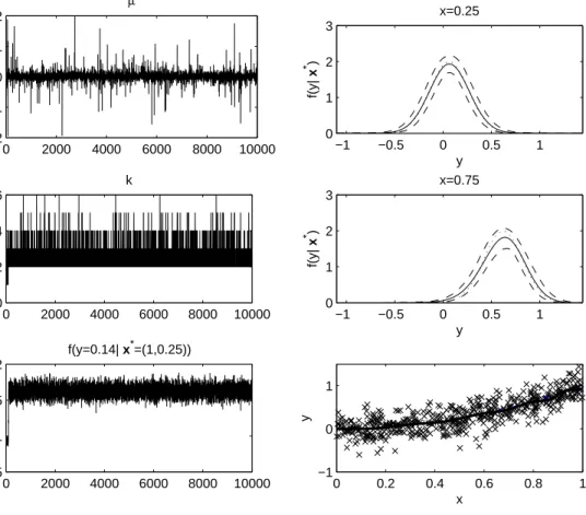
variance 0.04,N(yi;x2i1,0.04). The data were analyzed using a mixture of normals with the prior specification of Section 2.5.1, and with the MCMC algorithm of Section 2.4 implemented for 10,000 iterations, discarding the initial 1,000 iterations as a burn-in. Figure 2.1 shows selected results. The algorithm converged rapidly and mixing was good based on trace plots of µ, the number of clusters, andf(y= 1.5|x∗ _{= (1 0}_.₂₅₎0_{), where the data point for y is randomly selected}

among possible values (the left panel of Figure 2.1). As shown in the right panel of Figure 2.1, the predictive densities and mean function of y (solid lines) well approximate the true values (dotted lines), which are completely embedded within pointwise 99% credible intervals (dashed lines). The posterior mean of the number of clusters was 2.4 with a 95% credible interval of [2,4] and the estimated normal means were almost equally spaced over (0,1).

As a more challenging second simulation case, we simulated data to approximately mimic the data in the reproductive epidemiology study considered in Section 2.6. In particular, we

(39)

0 2000 4000 6000 8000 10000 −2 −1 0 1 2 µ

0 2000 4000 6000 8000 10000 0

2 4 6

k

0 2000 4000 6000 8000 10000 0.5

1 1.5 2

f(y=0.14| x*=(1,0.25))

−1 −0.5 0 0.5 1 0 1 2 3 f(y| x * ) y x=0.25

−1 −0.5 0 0.5 1 0 1 2 3 f(y| x * ) y x=0.75

0 0.2 0.4 0.6 0.8 1 −1

0 1

x

y

FIGURE 2.1: Results for the first simulation example. The left column provides trace plots for representative quantities, while the right panel shows the conditional distributions for two different values of x, as well as the mean function estimation along with the raw data. Posterior means are solid lines, pointwise 99% credible intervals are dashed lines, and true values are dotted lines.

generated data from the following mixture of two linear models:

f(yi|xi) = (1−xi41)N(yi; 1,0.04) +x4i1N(yi;,1−x2i1,0.01),