PRIORITIZATION IN SERVICE SYSTEMS WITH NONLINEAR DELAY COSTS
Huiyin Ouyang
A dissertation submitted to the faculty of the University of North Carolina at Chapel Hill
in partial fulfillment of the requirements for the degree of Doctor of Philosophy in the
Department of Statistics and Operations Research.
Chapel Hill
2016
Approved by:
Nilay T. Argon
Vidyadhar G. Kulkarni
Haipeng Shen
ABSTRACT
Huiyin Ouyang: Prioritization in Service Systems with Nonlinear Delay Costs
(Under the direction of Nilay T. Argon and Serhan Ziya)
ACKNOWLEDGEMENTS
I would like to express my special appreciation and thanks to my advisors, Dr. Nilay Argon and
Dr. Serhan Ziya, who have been encouraging me and helping me during my study, and providing
valuable advice for my research and career. I would also like to thank all my committee members,
Dr. Vidyadhar Kulkarni, Dr Nur Sunar, and Dr. Haipeng Shen for serving in my committee and
their comments and suggestions on my work.
TABLE OF CONTENTS
LIST OF TABLES . . . .
x
LIST OF FIGURES . . . xi
CHAPTER 1: INTRODUCTION . . . .
1
CHAPTER 2: PRIORITY ASSIGNMENT IN AN M/G/1 QUEUE WITH
NON-LINEAR WAITING COSTS . . . .
4
2.1
Introduction . . . .
4
2.2
Model description . . . .
6
2.3
Comparison of FCFS and fixed priority policies – general cost structures . . . .
7
2.4
Comparison of FCFS and fixed priority policies – polynomial cost functions . . . 11
2.4.1
Quadratic cost functions for both customer types . . . 12
2.4.2
Quadratic cost for one type and general cost for the other type . . . 17
2.4.3
Linear cost for one type and general cost for the other type . . . 20
2.4.4
Discussions . . . 21
2.5
Comparison of FCFS and fixed priority policies – exponential convex cost functions . . 22
2.5.1
General service time distributions . . . 23
2.5.2
Exponential service times with identical rates for both types . . . 24
2.6
Convex cost functions . . . 27
2.7
Concave cost functions . . . 28
2.7.1
Comparison of LCFS and fixed priority policies . . . 28
2.7.2
Waiting time LSTs . . . 29
2.7.3
Exponential cost function . . . 30
2.8.1
Same service rates . . . 32
2.8.1.1
Quadratic cost functions . . . 32
2.8.1.2
Exponential cost functions . . . 34
2.8.2
Different service rates . . . 35
2.8.2.1
Quadratic cost functions . . . 35
2.9
Conclusions . . . 36
CHAPTER 3: ALLOCATION OF INTENSIVE CARE UNIT BEDS DURING
PE-RIODS OF HIGH DEMANDS . . . 38
3.1
Introduction . . . 38
3.2
Literature review . . . 40
3.3
Model Description . . . 43
3.4
Single-bed ICU . . . 47
3.5
Analysis of the multi-bed ICU model . . . 49
3.5.1
Formulation of the discounted model . . . 49
3.5.2
Main results for the discounted model . . . 50
3.5.2.1
Optimality of non-idling ICU beds. . . 51
3.5.2.2
General structure of the optimal policy. . . 52
3.5.2.3
Conditions for the optimality of a state independent policy. . . 53
3.5.3
Long-run average cost criteria . . . 54
3.6
Numerical study . . . 57
3.6.1
A new policy and other benchmarks . . . 59
3.6.2
Results of the numerical study . . . 60
3.7
Conclusions . . . 62
CHAPTER 4: PRIORITIZATION IN A MULTI-SERVER QUEUEING SYSTEM
WITH IMPATIENT CUSTOMERS . . . 65
4.1
Introduction . . . 65
4.2
Literature Review . . . 66
4.3.1
Model description . . . 67
4.3.2
Formulation as an MDP . . . 68
4.4
Main results for the discounted model . . . 71
4.4.1
Conditions for optimality of non-idling policies . . . 72
4.4.2
Optimality of State-independent priority policies . . . 74
4.5
Main results for the average model . . . 75
4.6
Analysis of three special models . . . 75
4.6.1
Special model I: no queueing . . . 75
4.6.2
Special model II: no transitions between stages . . . 76
4.6.3
Special model III: Stage changes in one direction only while in queue . . . 78
4.7
Numerical study . . . 78
4.7.1
Switching curve . . . 79
4.7.2
Compare the performance of some priority index policies . . . 80
4.7.2.1
Single scenario comparison . . . 82
4.7.2.2
Random comparisons . . . 82
4.8
Conclusions . . . 84
CHAPTER 5: CONCLUSIONS . . . 86
APPENDIX A: PROOFS OF RESULTS IN CHAPTER 2 . . . 88
A.1 Proof of Results in Section 2.2 . . . 88
A.2 Proof of results in Section 2.3 . . . 89
A.3 Laplace-Stieltjies transforms (LSTs) of the busy period and waiting times
under FCFS and fixed priority policies . . . 91
A.4 Proof of results in Section 2.4 . . . 92
A.5 Proof of results in Section 2.5 . . . 100
A.6 Proof of results in Section 2.6 . . . 101
A.7 Proof of results in Section 2.7 . . . 102
APPENDIX B: PROOFS OF RESULTS IN CHAPTER 3 . . . 106
B.1.1
Proof of Proposition 3.1 . . . 106
B.1.2
Proof of Corollary 3.1 . . . 110
B.2 Proofs of the Results in Section 3.5 . . . 111
B.2.1
Proof of Proposition 3.2 . . . 111
B.2.2
Proof of Proposition 3.3 . . . 114
B.2.3
Proof of Proposition 3.4 . . . 126
B.2.4
Proof of Theorem 3.1 . . . 137
B.2.5
Proof of Theorem 3.2 . . . 139
B.2.6
Proof of Theorem 3.3 . . . 141
APPENDIX C: PROOFS OF RESULTS IN CHAPTER 4 . . . 143
C.1 Proof of results in Section 4.4 . . . 143
LIST OF TABLES
2.1
The threshold values (
A
and
B
) to characterize the best policy among
F, P F
1and
P F
2.
. . . 33
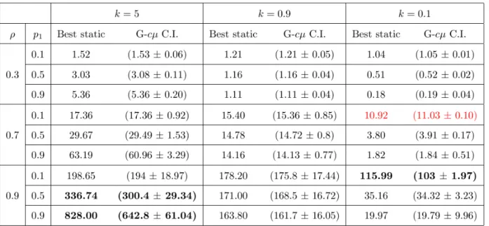
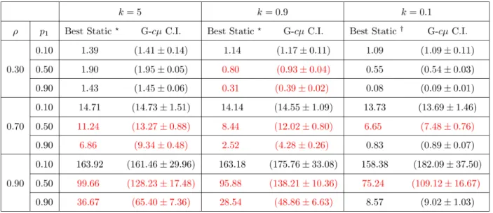
2.2
Compare the best static policy with G-
cµ
rule under quadratic cost . . . 33
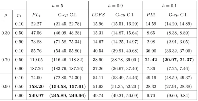
2.3
Compare the best static policy with G-
cµ
rule under exponential cost (10
−2) . . . 34
2.4
The threshold values (AandB) for different service rates.. . . 35
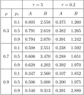
2.5
Compare the best static policy with G-
cµ
rule under quadratic costs with
τ
= 5 . . . 36
2.6
Compare the best static policy with G-
cµ
rule under quadratic costs with
τ
= 0
.
2 . . . 36
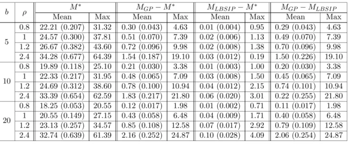
3.1
Performance comparison of the optimal policy, GP, and LBSIP. (All
num-bers are in percentages. In the columns titled “Mean” the first number
reported is the mean, the second number is the 95% C.I. half-width.) . . . 61
4.1
Priority index policies and corresponding index . . . 81
4.2
Priority indices for the base scenario. . . 82
4.3
Computations of the priority indices for several scenarios . . . 82
4.4
Comparisons of the static policies and the optimal policy . . . 83
LIST OF FIGURES
2.1
Plots of
A
and
B
with respect to
λ
for exponential service times . . . 13
2.2
Plots of
A
and
B
with respect to
p
1for exponential service times . . . 15
2.3
Plots of
a
2and
b
1with respect to
ρ
and
p
2. . . 26
2.4
Plots of
a
2and
b
1with respect to
h
2. . . 26
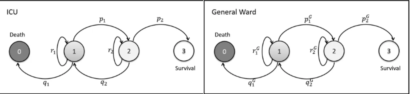
3.1
Transition diagram of patient evolution in the ICU and general ward . . . 44
4.1
Customer Transition Diagrams . . . 68
4.2
Optimal policy structure . . . 79
4.3
Changes of the switching curve in
µ
1,
R
1, and
β
1. . . 80
CHAPTER 1: INTRODUCTION
In many service systems customers are heterogeneous in that they have different service
require-ments and incur different costs. An interesting problem to the service provider is how to control
the service process by prioritizing service, and admitting or rejecting customers so that some
per-formance measure is optimized. For example, the director of an emergency department (ED) at a
hospital prioritizes the treatment of more severe patients to minimize the overall mortality rate. A
call center manager reserves several lines to serve more valued customers since these customers will
incur larger cost if they are unsatisfied. Hospital bed managers face the decision of how to allocate
beds when the demand exceeds their capacity, e.g., they either discharge an existing patient to
admit a new patient, or they reject the new patient. All these service systems provide services to
different types of customers, and their decisions are associated with prioritizing some customers
over others.
There is a vast literature that investigates models when the cost of holding customers in the
system are linear in their waiting time, and the optimal policies for these models are proved to be a
priority index rule. However, the costs in reality usually have more complicated structures that are
difficult to capture by a simple linear waiting cost approximation. For example, the health state of
ED patients does not in general deteriorate at a constant rate. On the other hand in certain cases,
it is even not appropriate to capture the cost structure as a function of waiting times. For example
in a hospital ward, the cost will depend on the medical outcome of the patients after his/her stay
in the ward, which may be indirectly related to waiting times. However, it is difficult to express
the cost as a direct function of waiting times in this case.
In the first part of this dissertation, we consider a single server queueing system with two
different types of customers. Each customer incurs a cost depending on its type and its waiting
time in the queue. The cost functions are assumed to be non-decreasing in the waiting time. Our
objective is to minimize the long-run average cost by controlling the order of service for customers
in the queue. The waiting costs for different types of patients are different, and also they are not
linear in the waiting time. In general, it is very difficult to keep track of the waiting times of all
customers in the system, or these kind of information may be very expensive or even impossible
to collect in practice. Hence, we are interested in finding “good” policies that do not need such
information under nonlinear costs.
The second part of this dissertation is motivated by the admission and discharge decisions given
in the intensive care units (ICUs) in hospitals. When a patient arrives to an ICU that is full, the
ICU director needs to decide either rejecting this new patient (by way of transfer to some other
ward or hospital) or discharging (transferring) an existing patient to make space for this one. In
an ICU setting, we are concerned about the dying probabilities of all patients, which can hardly
be approximated by a linear function.
In our model, the heterogeneity of ICU patients is in the sense of patients’ severity conditions,
and the severity conditions of patients could change during their stay in the hospital. We use
different stages to model the different health conditions of the patients, and we use a transition
matrix to represent the change of patient stages in the ICU. When patients are not in the ICU
either due to being early discharged or being rejected upon arrival, they will stay at some non-ICU
care place such as general wards, nursery rooms or even home, which we all refer as “the general
ward” throughout the dissertation. The stages of patients in such places will change according to
a similar pattern with different parameters from the transition matrix in ICU. The patients could
leave with an undesired outcome, e.g., death or readmission to ICU. Our objective is to minimize
the expected probability of such an undesired outcome by choosing which patients to keep in the
ICU.
become better or worse during the processing. The quality of completed jobs depends on which
stage they are finished with, and our objective is to maximize the total output quality by assigning
priorities, where jobs with lower priority will be processed by the general resource when the efficient
resources are all occupied.
CHAPTER 2: PRIORITY ASSIGNMENT IN AN M/G/1 QUEUE WITH
NONLINEAR WAITING COSTS
In this Chapter, we consider a single server queueing system with two different types of
cus-tomers. Each customer incurs a cost depending on its type and waiting time in the queue, which
is assumed to be non-decreasing and nonlinear. We would like to compare the performances of
several static policies.
2.1 Introduction
We consider a queueing system with two types of customers. For example, consider an
emer-gency room with patients who are more severely injured and those who only have small problems.
We assume that each customer incurs a waiting cost that depends on its type and the amount
of time it spends in the queue before its service starts. We also assume that the cost function is
increasing in time spent in the queue. The inter-arrival times and the service times depend on the
type as well. Our objective is to determine the best “static” policy that minimizes the long-run
average cost. By static policies, we mean policies that are independent of the state of the system,
such as priority policies that give priority to a certain type of customers or non-priority policies
like first-come-first-serve (FCFS) or last-come-first-serve (LCFS).
Then the problem that which type of customers should be prioritized was studied. For linear
cost functions when the cost is proportional to the delay, Cox and Smith (1961) first established
the optimality of the so called “
cµ
-rule” for M/G/1. According to the
cµ
-rule, customers with
larger
c
iµ
iindex are assigned higher priority, where
c
iis the per unit time waiting cost and
µ
iis
the service rate for type
i
customers, to minimize the long-run average waiting cost in the system.
Many other work has been done under the assumption of linear cost functions.
The consideration of nonlinear costs is necessary because approximating customers’ delay
sensi-tives with a linear function may not be reasonable in practice. For example, when perishable items
wait for service, or landing aircraft wait in the air for landing, etc., the cost of a unit delay cannot
be constant as delay increases, because in the former case, the items lose value, and in the latter
case, the aircraft may fail for lack of fuel. Dewan and Mendelson (1990) provided a more detailed
discussion about the delay cost structures. A number of papers have considered the generalized
cost functions in their queueing models. Af´
eche and Mendelson (2004) compared the
revenue-maximizing and socially optimal equilibria under uniform pricing, preemptive, and nonpreemptive
priority auctions with an admission price and a generalized delay cost structure. Hassin et al.
(2009) showed that relative priorities in an n-class queueing system can reduce customer waiting
costs in a single server Markovian model where the goal is to minimize a non-linear cost function
of class expected waiting times. Rothkopf and Smith (1984) conjectured that no static priority
policy would minimize the expected delay costs when delay cost functions are nonlinear. Haji and
Newell (1971) showed that when the cost functions are convex increasing functions, the optimal
strategy will always involve serving customers of the same type according to the FCFS discipline.
Van Mieghem (1995) proved that when waiting costs are convex in time, a generalized version of
the
cµ
-rule is asymptotically optimal under heavy traffic. Mandelbaum and Stolyar (2004) also
proved the heavy-traffic optimality of the generalized
cµ
-rule under more general settings.
The generalized
cµ
-rule is actually a dynamic policy that gives priority to the customer who
has the largest
C
i0(
t
)
µ
ivalue in the system at every service completion epoch, where
C
i(
t
) is the
policies, such as the FCFS and LCFS policies and priority policies that give priority to customers
according to their types without considering their waiting times in the system.
The remainder of this article is organized as follows. We describe our model in Section 2.2, then
in Section 2.3 we provide analytical comparisons of the three commonly used static policies, namely
F
,
P F
1and
P F
2, whereF
denotes first-come-first-serve (FCFS) and
P F
idenotes the priority policy
that prioritizes type
i
customers and employs FCFS within each type for
i
= 1
,
2. We apply our
results for polynomial cost functions in Section 2.4 and for exponential convex function in Section
2.5, then we give a theoretical result that shows when the cost functions are convex, we only need
to compare
F
,
P F
1and
P F
2in Section 2.6. We provide similar results when comparing policies
L
,
P L
1and
P L
2, where
L
denotes last-come-first-serve (LCFS), and
P L
idenotes the priority policy
that prioritizes type
i
customers and employs LCFS within each type for
i
= 1
,
2, and proved that
it suffices to compare only
L
,
P L
1and
P L
2when the cost functions are concave. By means of
a numerical study, we compare the best static policy that we found in earlier sections with the
generalized
cµ
-rule in Section 2.8. Finally, Section 2.9 provides our conclusions.
2.2 Model description
Consider a single server queueing system with two types of customers. Customers arrive to the
system according to a Poisson process with rate
λ >
0, and each arriving customer belongs to type
i
∈ {
1
,
2
}
with probability
p
i>
0, where
p
1+
p
2= 1, independent of the arrival process. Service
times for type
i
∈ {
1
,
2
}
customers are independent and identically distributed (i.i.d.) with mean
τ
i>
0 and second moment
ξ
i>
0. We define
ρ
i≡
p
iλτ
iand
ρ
≡
ρ
1+
ρ
2, which we call the system
load, and we assume that
ρ <
1 for stability. Each type
i
customer incurs a waiting cost
C
i(
t
)
when its waiting time in the queue is
t
, for
t
≥
0 and
i
= 1
,
2. We assume that
C
i(
t
) is first-order
differentiable and non-decreasing in
t
for fixed
i
.
be completed without any preemption before the server moves onto serving another customer. We
let Π denote the set of all such queueing policies.
For any policy
π
∈
Π, define the long-run average cost as
C
π≡
lim
t→∞P
2i=1
P
ni(t)k=1
C
i(
V
π,x0 i,k
)
t
,
(2.1)
where
n
i(
t
) is the number of type
i
customers that has arrived to the system by time
t
and
V
i,kπ,x0is the waiting time of the
k
th arriving type
i
customer under policy
π
and initial state
x
0. Our
objective is to identify policies that provide the smallest long-run average waiting cost
C
πin the
policy set Π for any given initial state
x
0. LetW
iπdenote the steady-state waiting time of a type
i
customer under policy
π
, then we will show in Appendix A that if
E
h
C
i(
W
iπ)
i
exists for both
i
∈ {
1
,
2
}
,
C
πdefined in (2.1) satisfies
C
π=
λp
1E
h
C
1(
W
1π)
i
+
λp
2E
h
C
2(
W
2π)
i
.
(2.2)
2.3 Comparison of FCFS and fixed priority policies – general cost structures
In this section, we present the comparison of three commonly used policies within Π, namely
F
,
P F
1and
P F
2. In order to compare
C
F,
C
P F1and
C
P F2, we need several definitions and lemmas.
Definition 2.1.
(E.g., Shaked and Shanthikumar (2007)). Let
X
and
Y
be two random variables
with corresponding cumulative distribution functions
F
X(
·
) and
F
Y(
·
). If
F
X(
x
)
≥
F
Y(
x
) for all
x
∈
(
−∞,
∞
), then
X
is said to be smaller than
Y
in the usual stochastic ordering (denoted by
X
≤
stY
).
Definition 2.2.
(Di Crescenzo (1999)). Let
X
and
Y
be two non-negative random variables with
X
≤
stY
and
E
[
X
]
< E
[
Y
]
<
∞
. Then, we write
Z
≡
Ψ(
X, Y
) to mean that
Z
is a random
variable with probability density function
f
Z(
x
) =
F
X(
x
)
−
F
Y(
x
)
where
F
X(
·
) and
F
Y(
·
) are the cumulative distribution functions of
X
and
Y
, respectively.
Di Crescenzo (1999) shows that
f
Z(
x
) is a probability density function.
Lemma 2.1.
(Theorem 4.1 of Di Crescenzo (1999)) Let
X
and
Y
be two non-negative random
variables satisfying
X
≤
stY
and
E
[
X
]
< E
[
Y
]
<
∞, and let
Z
= Ψ(
X, Y
)
.
Let also
g
be
a measurable and differentiable function such that
E
[
g
(
X
)]
and
E
[
g
(
Y
)]
are finite, and let its
derivative
g
0be measurable and Riemann-integrable on the interval
[
x, y
]
for all
0
≤
x
≤
y. Then,
E
g
0(
Z
)
is finite and
E
[
g
(
Y
)]
−
E
[
g
(
X
)] =
E
[
g
0(
Z
)]
E
[
Y
]
−
E
[
X
]
.
Lemma 2.1 presents a probabilistic analogue of the mean value theorem, where
Z
is a random
variable that can be considered as the “mean value” of
X
and
Y
. However, unlike for the
(deter-ministic) mean value theorem,
Z
does not change with the function
g
, and
Z
= Ψ(
X, Y
) is not
necessarily ordered (in some stochastic sense) between
X
and
Y
. For example, when
X
and
Y
are
exponential random variables with distinct rates,
Z
=
stX
+
Y
(see Example 3.1 in Di Crescenzo
(1999)).
We will use Lemma 2.1 in several of our results including our main result that compares
C
F,
C
P F1and
C
P F2. Before we present this result, we need two more lemmas for the comparison of
W
iF,
W
P Fii
,
W
P Fi3−i
for
i
= 1
,
2.
Lemma 2.2.
(E.g., Gross et al. (2008) and Miller (1960)) For an M/G/1 queueing sysem, the
expected steady-state waiting times under FCFS and
P F
iare given as follows:
E
[
W
F] =
λ
¯
ξ
2(1
−
ρ
)
,
E
[
W
P Fi
i
] =
λ
ξ
¯
2(1
−
ρ
i)
,
E
[
W
P Fi 3−i] =
λ
ξ
¯
2(1
−
ρ
i)(1
−
ρ
)
,
where
ξ
¯
=
p
1ξ
1+
p
2ξ
2, and we drop the subscript in
W
iFsince the distribution of
W
Fdoes not
depend on
i.
Lemma 2.3.
For fixed
i
= 1
,
2
, we have
W
P Fii
≤
stW
F≤
stW
3−P Fii.
for the non-priority type under a priority policy and greater than those for the priority type. Lemma
2.3 specifies a type of stochastic ordering between these three steady-state random variables.
Based on Lemmas 2.2 and 2.3, for
i
∈ {
1
,
2
},
we define the following random variables,
U
P Fii
≡
Ψ(
W
P Fii
, W
F) and
U
P Fi3−i
≡
Ψ(
W
F, W
P Fi 3−i)
.
Note that
U
P Fij
is well defined for
i, j
∈ {
1
,
2
}
because
W
P Fii
≤
stW
F≤
stW
P F3−ii
according to
Lemma 2.3, and when
ρ <
1 and
p
i>
0, we have
E
W
P Fii
< E
W
F< E
W
P F3−ii
<
∞
, for
i
= 1
,
2 by Lemma 2.2.
Our main results are all stated under the following assumption.
Assumption 2.1.
For fixed
i
∈ {
1
,
2
}
,
E
h
C
i(
W
iπ)
i
exists for
π
∈ {F, P F
1, P F
2}
.
We are now ready to present our main result and an immediate corollary
Theorem 2.1.
Under Assumption 2.1, we have,
(a) for
i
= 1
,
2
,
C
F≤
C
P Fiif and only if
a
i≤
b
i,
where
a
i≡
E
C
i0(
U
P Fii
)
τ
i, b
i≡
E
C
3−0 i(
U
P Fi 3−i)
τ
3−i.
(2.4)
(b)
C
P F1≤
C
P F2if and only if
(1
−
ρ
1)(
a
2−
b
2)
≤
(1
−
ρ
2)(
a
1−
b
1)
.
Corollary 2.1.
(a) If
a
1≤
b
1and
a
2≤
b
2, then
C
F≤
C
P F1and
C
F≤
C
P F2.
(b) For fixed
i
∈ {
1
,
2
}, if
a
i≥
b
iand
a
i−
b
i1
−
ρ
i≥
a
3−i−
b
3−i1
−
ρ
3−i,
then
C
P Fi≤
C
Fand
C
P Fi≤
C
P F3−i.
Corollary 2.1 provides necessary and sufficient conditions for the optimality of
F
,
P F
1and
P F
2within the set of these three policies. These conditions require computation of
a
iand
b
ifor
i
= 1
,
2.
In order to compute
a
iand
b
iin Theorem 2.1 and Corollary 2.1, we need to obtain
E
h
C
i0(
U
P Fji
)
i
for
i, j
∈ {
1
,
2
}
. In some situations, the cost functions may be simple for one type and complicated
for the other type. For example, we may assume that the cost function for type 2 customers is
linear or quadratic, and the cost function for type 1 customers has a more complicated structure.
In this case, we can use the next two results to order
C
F,
C
P F1and
C
P F2without computing
E
h
C
10(
U
P Fj 1)
i
, but by computing
E
h
C
20(
U
P Fji
)
i
for
i, j
∈ {
1
,
2
}.
Corollary 2.2.
(a) If
C
10(
t
)
≥
τ
1max
{a
2, b
1}
for all
t
≥
0
, then
C
P F1≤
C
F≤
C
P F2.
(b) If
C
10(
t
)
≤
τ
1min
{a
2, b
1}
for all
t
≥
0
, then
C
P F2≤
C
F≤
C
P F1.
(c) If
τ
1a
2≤
C
10(
t
)
≤
τ
1b
1for all
t
≥
0
, then
C
F≤
C
P F1and
C
F≤
C
P F2.
Corollary 2.3.
If
E
[
C
20(
U
P F21
)]
6
= 0
and
E
[
C
20(
U
P F1
1
)]
6
= 0
, define
α
≡
τ
1E
[
C
02
(
U
2P F2)]
τ
2E
[
C
20(
U
P F2
1
)]
and
β
≡
τ
1E
[
C
02
(
U
2P F1)]
τ
2E
[
C
20(
U
P F1
1
)]
.
(a) If
C
10(
t
)
≥
max
{α, β}C
20(
t
)
for all
t
≥
0
, then
C
P F1≤
C
F≤
C
P F2.
(b) If
C
10(
t
)
≤
min
{α, β}C
20(
t
)
for all
t
≥
0
, then
C
P F2≤
C
F≤
C
P F1.
(c) If
αC
20(
t
)
≤
C
10(
t
)
≤
βC
20(
t
)
for all
t
≥
0
, then
C
F≤
C
P F1and
C
F≤
C
P F2.
Corollary 2.2 compares
C
10(
t
) with two fixed quantities,
τ
1a
2and
τ
1b
1, for allt
≥
0. Hence
C
10(
t
) has to be bounded from either above or below to be able to apply this result as in the case of
a linear or logarithmic cost function for type 1 customers. On the other hand, in Corollary 2.3, we
compare
C
10(
t
) with two time-varying quantities,
αC
20(
t
) and
βC
20(
t
), and hence
C
10(
t
) does not need
to be bounded. However, in Corollary 3, we require that
E
h
C
20(
U
P Fi1
)
i
2.4 Comparison of FCFS and fixed priority policies – polynomial cost functions
In this section, we focus on the case where the cost function for at least one type of customer
is polynomial. In particular, suppose that for some
i
= 1
,
2,
C
i(
t
) =
j(i)X
l=1
h
l(
i
)
t
l,
(2.5)
where
j
(
i
) is the (finite) degree of the polynomial function
C
i(
t
), and
h
l(
i
) are some real numbers
such that
C
i0(
t
)
≥
0 for all
t
≥
0. We first provide conditions under which Assumption 2.1 holds
the polynomial cost functions in Lemma 2.4 (the proof is provided in Appendix A).
Lemma 2.4.
Assumption 2.1 is satisfied for
C
i(
t
)
that takes the form of
(2.5)
if
ρ <
1
, and the
first
(
j
(
i
) + 1)
moments of service times for both types are finite.
In order to apply Theorem 2.1 and Corollaries 2.1, 2.2 and 2.3, we need to compute
E
h
C
i0(
U
P Fmk
)
i
for some
i, k, m
∈ {
1
,
2
}
, where
E
h
C
i0(
U
P Fmk
)
i
=
j(i)
X
l=1
lh
l(
i
)
E
U
P Fmk
l−1.
(2.6)
Here,
E
U
P Fmk
l−1for
l
= 1
, . . . , j
(
i
) can be computed as
E
U
P Fmk
l−1=
E
(
W
F)
l−
E
(
W
P Fmk
)
ll
E
[
W
F]
−
E
[
W
P Fmk
]
,
(2.7)
by letting
g
(
x
) =
x
l/l
in Lemma 2.1. See Appendix A for the proof of (2.6).
2.4.1 Quadratic cost functions for both customer types
Suppose that
C
i(
t
) =
k
it
2+
h
it
, where
k
i, h
i≥
0 and
i
∈ {
1
,
2
}
. Let
ζ
idenote the third moment
of the service times for type
i
∈ {
1
,
2
}
and ¯
ζ
≡
p
1ζ
1+
p
2ζ
2. Then, we show in Appendix A that
a
i=
k
iτ
i2 ¯
ζ
3 ¯
ξ
+
λ
ξ
¯
1
−
ρ
+
λp
iξ
i1
−
ρ
i+
ξ
3−iτ
3−i+
h
iτ
i,
(2.8)
b
i=
k
3−iτ
3−i2 ¯
ζ
3 ¯
ξ
1 +
1
1
−
ρ
i+
λ
ξ
¯
1
−
ρ
1 +
1
1
−
ρ
i+
ξ
iτ
i(1
−
ρ
i)
2+
h
3−iτ
3−i.
(2.9)
When we compare
a
i’s and
b
i’s given above, we found that for
i
= 1
,
2,
b
3−i−
a
i=
k
iτ
i2 ¯
ζ
3 ¯
ξ
(1
−
ρ
3−i)
+
λ
¯
ξρ
3−i1
−
ρ
1
1
−
ρ
3−i+
1
1
−
ρ
i+
λp
3−iξ
3−i1
(1
−
ρ
3−i)
2+
1
1
−
ρ
i+
1
1
−
ρ
3−i≥
0
,
(2.10)
because
ρ, ρ
1, ρ
2<
1 and all moments of service times are non-negative. Therefore, when both cost
functions are quadratic, if
a
i> b
ifor some
i
= 1
,
2 (and thus
a
3−i≤
b
i< a
i≤
b
3−i), then
P F
iis
the best among
F
,
P F
1and
P F
2according to Corollary 2.1(b); otherwise (
a
1≤
b
1and
a
2≤
b
2),
F
is the best among
F
,
P F
1and
P F
2by Corollary 2.1(a). By comparing
a
iand
b
ifor fixed
i
∈ {
1
,
2
}
,
we find that
a
i≥
b
i(and thus
P F
iis the best), if and only if
k
iτ
i≥
k3−i
τ3−i
h
2−ρi 1−ρi
2 ¯ζ
3 ¯ξ
+
λξ¯1−ρ
+
λpiξi 1−ρi+
ξiτi
i
+
h3−iτ3−i
−
hi
τi
h
2 ¯ζ
3 ¯ξ
+
λξ¯1−ρ
+
λpiξi 1−ρi+
ξ3−i
τ3−i
i
.
(2.11)
Hence, using Corollary 2.1 and Equations (2.8) and (2.9), we were able to obtain a complete order
of policies
F
,
P F
1and
P F
2when cost functions are quadratic. To gain further insights, we next
consider the case that
h
1/τ
1=
h
2/τ
2, e.g., whenC
i(
t
) =
k
it
2for
i
= 1
,
2, in the remainder of this
section.
k
1/k
2> Bτ
1/τ
2, and
F
is the best if
Aτ
1/τ
2≤
k
1/k
2≤
Bτ
1/τ
2, where
A
≡
2 ¯ζ3 ¯ξ
+
λξ¯1−ρ
+
λp2ξ21−ρ2
+
ξ1 τ12−ρ2
1−ρ2
2 ¯ζ
3 ¯ξ
+
λξ¯1−ρ
+
λp2ξ21−ρ2
+
ξ2 τ2<
2−ρ11−ρ1
2 ¯ζ
3 ¯ξ
+
λξ¯1−ρ
+
λp1ξ11−ρ1
+
ξ1 τ12 ¯ζ
3 ¯ξ
+
λξ¯1−ρ
+
λp1ξ11−ρ1
+
ξ2 τ2≡
B.
Proposition 2.1 completely characterized the best policy among
F
,
P F
1and
P F
2for quadratic
cost functions with
h
1/τ
1=
h
2/τ
2. In particular, it provides thresholds on
k
1/k
2such that
P F
1is
the best if
k
1/k
2is large,
P F
2is the best if
k
1/k
2is small and
F
is the best if
k
1/k
2is medium.
Proposition 2.1 also provides some useful insights.
For example, when
λ
→
1
/
τ
¯
, where ¯
τ
=
p
1τ
1+
p
2τ
2is the mean service time, we find that
A
→
1−2−ρρ22and
B
→
2−1−ρρ11, then in heavy traffic
F
is preferred when
k
1and
k
2are not significantly different.
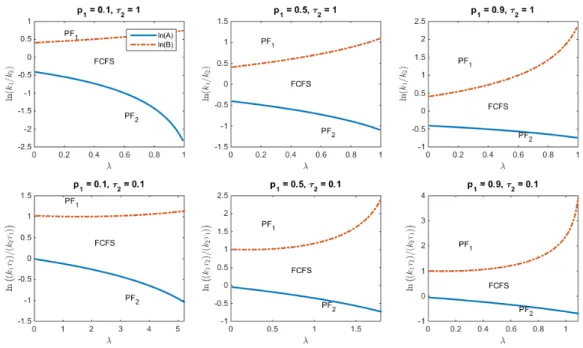
Figure 2.1 provides plots of ln
A
and ln
B
with respect to
λ
, from which we can observe the
above insights. We assume that the service times are exponentially distributed, and
τ
1= 1.
Figure 2.1: Plots ofAandB with respect to λfor exponential service times
Proposition 2.2.
A
decreases in
λ
if and only if
ξ
2τ
2−
(2
−
ρ
2)
ξ
1(1
−
ρ
2)
τ
1<
p2τ2
(1−ρ2)2
2 ¯ζ
3 ¯ξ
+
λξ¯1−ρ
+
λp2ξ21−ρ2
2 ¯ζ
3 ¯ξ
+
λξ¯1−ρ
+
λp2ξ21−ρ2
+
ξ1 τ1¯
ξ
(1−ρ)2
+
p2ξ2(1−ρ2)2
,
(2.12)
and
B
increases in
λ
if and only if
ξ
1τ
1−
(2
−
ρ
1)
ξ
2(1
−
ρ
1)τ
2<
p1τ1
(1−ρ1)2
2 ¯ζ
3 ¯ξ
+
λξ¯1−ρ
+
λp1ξ11−ρ1
2 ¯ζ
3 ¯ξ
+
λξ¯1−ρ
+
λp1ξ11−ρ1
+
ξ2 τ2¯
ξ
(1−ρ)2
+
p1ξ1(1−ρ1)2
.
(2.13)
Proposition 2.2 provides conditions under which the thresholds for the optimality of these
policies monotonically change with
λ
. Note that the right-hand side of (2.12) and (2.13) are both
nonnegative, which then give a sufficient condition, i.e., if
ξ1τ1
>
ξ2(1−ρ2)
τ2(2−ρ2)
, then
A
decreases in
λ
and
if
ξ1 τ1<
(2−ρ1)ξ2
(1−ρ1)τ2
, then
B
increases in
λ
. If
ξ1 τ1<
ξ2(1−ρ2)
τ2(2−ρ2)
, the left-hand side of (2.12) is positive
and the right-hand converges to 0 as
p
2→
0, thus (2.12) may not hold for very small
p
2and
A
increases in
λ
, which means
P F
2is preferred for a larger range of values of
k
1/k
2as
λ
increases.
Similarly if
ξ1τ1
>
(2−ρ1)ξ2
(1−ρ1)τ2
, we notice that
B
decreases in
λ
when
p
1is sufficiently small, and thus
P F
1is preferred for a larger range of values of
k
1/k
2as
λ
increases.
Thus, we conclude that if the
proportion of one type of customers is sufficiently small, and the ratio of
ξ
i/τ
ifor the same type is
sufficiently large, then prioritizing that type becomes more preferable as
λ
increases.
On the other hand, if the ratios
ξ
1/τ
1and
ξ
2/τ
2are similar, e.g., when service times are i.i.d.
for all customers, then the interval (
A, B
) enlarges as
λ
increases, which indicates that
F
is more
preferable as the system becomes busier. However, this result is only to compare
F
with the fixed
priority policies, under which prioritization is always given to one type of customers irrespective of
the waiting times of customers. Under such a static priority rule, as the arrival rate increases, the
non-priority customers will wait much longer, resulting in a significant increase in waiting costs as
the cost increases at a higher rate for longer waiting. If we consider dynamic prioritization that
takes into account the waiting times of customers, then
F
may not perform as well as a dynamic
priority rule as we illustrate later by a numerical study in Section 2.8.
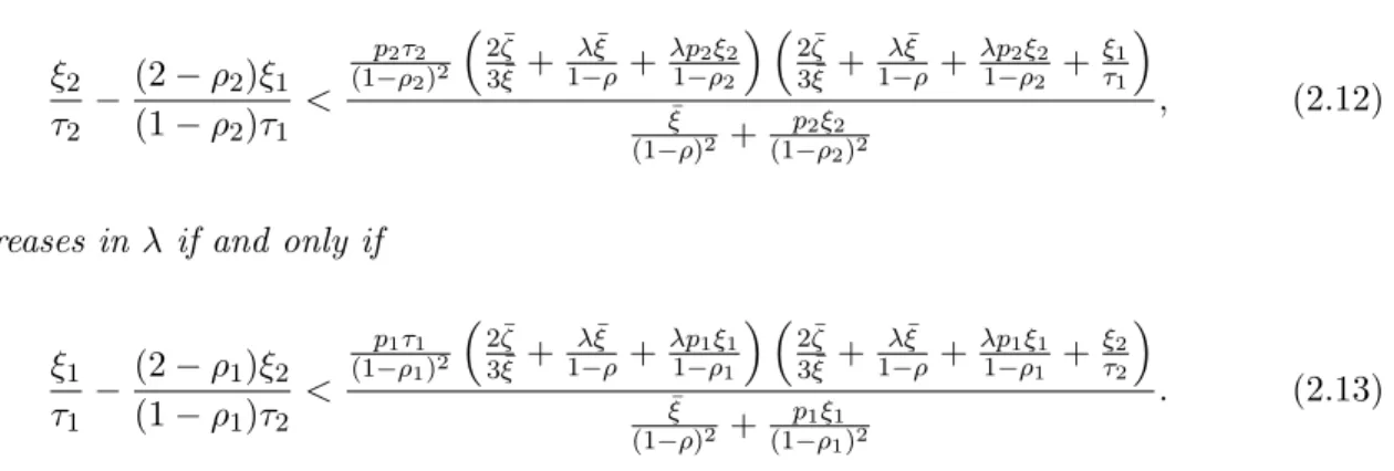
Figure 2.2: Plots ofA andB with respect top1for exponential service times
We notice from Figure 2.2 that when the mean service times are different,
A
and
B
do not
always change monotonically in
p
1. It is difficult to provide an algebraical analysis of how
A
and
B
change with respect to
p
i, given that ¯
ξ,
ζ, ρ
¯
and
ρ
iall change in
p
i. We can first look at the
heavy traffic setting, i.e., when
λ
→
1
/
τ
¯
. We have,
lim
p1→0 λ→1/τ2
A
= 0
,
lim
p1→0 λ→1/τ2
B
= 2
,
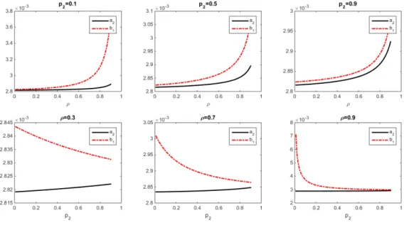
lim
p1→1 λ→1/τ1
A
=
1
2
,
plim
1→1 λ→1/τ1B
=
∞.
In words, we would not like to prioritize type
i
customers if the proportion of this type is close to
one under heavy traffic; on the other hand, if the proportion of type
i
customers is close to 0, we
would prioritize this type is preferred if
k
i/τ
i>
2
k
3−i/τ
3−i, and otherwise choose
F
under heavy
traffic.
Furthermore, if we assume that the service times are i.i.d., then, ¯
ξ,
ζ
¯
, and
ρ
no longer depend
on
p
i, and only
ρ
iwill change in
p
i. Our next result analyzes the monotonicity of
A
and
B
in
p
iunder such a setting.
Proposition 2.3 indicates that as the proportion of one type increases, giving priority to that
type is preferred for a smaller range of
k
1/k
2values, while prioritizing the other type is preferred
for a wider range of
k
1/k
2values. Intuitively, we would not like to prioritize type
i
customers if
their total load on the system is too large under quadratic waiting cost, since by prioritizing such
a large group, type 3
−
i
customers will wait much longer, resulting in a significant increase in
waiting costs. This intuition only works when service times are identical for all customers, and we
have numerical examples in Section 2.8 show that
A
and
B
do not necessarily increase in
p
1when
service times are different for the two types of customers.
When the service times are i.i.d., we have,
A
decreases in
λ
and increases in
p
1, and
B
increases
in both
λ
and
p
1from Propositions 2.2 and 2.3. Hence, we could obtain the range of values of
A
and
B
from their monotonicity. More specifically, we have
A >
lim
p1→0 λ→1/τ
A
= 0
,
and
A <
lim
p1→1 λ→0
A
=
2ζ3ξ
+
ξ τ4ζ
3ξ
+
ξ τ=
2
τ ζ
+ 3
ξ
24
τ ζ
+ 3
ξ
2,
and
B >
lim
p1→0 λ→0
B
=
4
τ ζ
+ 3
ξ
22
τ ζ
+ 3
ξ
2,
and
B <
plim
1→1 λ→1/τ
B
=
∞.
In the end of this section, we compare the values of
A
and
B
under two different service
time distributions. Let
A
exp[
B
exp] and
A
det[
B
det] denote the values of
A
[
B
] under exponential and
deterministic service times, respectively.
Proposition 2.4.
(a)
A
exp≤
A
detif and only if
τ
2≤
τ
1(2
−
ρ
2)
/
(1
−
ρ
2)
.
(b)
B
exp≥
B
detif and only if
τ
2≥
τ
1(1−
ρ
1)/
(2
−
ρ
1).
Proposition 2.4 implies that if
τ1 τ2∈
1−ρ2
2−ρ2
,
2−ρ1
1−ρ1
, then
A
exp≤
A
det< B
det≤
B
exp, and hence,
type is sufficiently faster to serve in the mean sense, say,
τ
1/τ
2>
(2
−ρ
1)
/
(1
−ρ
1), then
A
exp≤
A
detand
B
exp≤
B
det, which means that under exponential service times,
P F
2(prioritizing the slower
type) is preferred for a smaller range of values of
k
1/k
2, andP F
1(prioritizing the faster type) is
preferred for a wider range of values of
k
1/k
2than that under deterministic service times.
2.4.2 Quadratic cost for one type and general cost for the other type
Suppose one type of customers has a quadratic cost function (say,
C
2(
t
) =
k
2t
2+
h
2t
for
h
2, k
2≥
0), and the other type has a general cost function. In this section, we will demonstrate
how Corollaries 2.2 and 2.3 can be applied in such a case.
We first focus on Corollary 2.2. When
C
2(
t
) is a quadratic function,
a
2and
b
1are given by
(2.8) and (2.9), respectively, and hence we have
a
2≤
b
1from (2.10). Therefore, in Corollary 2.2,
we can replace max
{a
2, b
1}
with
b
1and min
{a
2, b
1}
with
a
2. Furthermore, sincea
2≤
b
1, we know
that the interval (
τ
1a
2, τ
1b
1) is not necessarily an empty set and hence part (c) of Corollary 2.2
could be applicable. Consequently, Corollary 2.2 implies that if the smallest marginal increase in
C
1(
t
) is at least
τ
1b
1, then type 1 customers should be prioritized; if the largest marginal increase
in
C
1(
t
) is at most
τ
1a
2, then type 2 customers should be prioritized; and if the marginal increase
in
C
1(
t
) lies between
τ
1a
2and
τ
1b
1at all times, then
F CF S
should be employed. Furthermore, by
Equations (2.8), (2.9) and (2.10), we notice that
a
i,
b
iand the difference
b
3−i−
a
iall increase in
λ
for
i
∈ {
1
,
2
}
since
ρ
i,
ρ
3−i, 1
/
(1
−
ρ
), 1
/
(1
−
ρ
i) and 1
/
(1
−
ρ
3−i) all increase in
λ
. This implies
that the bounds
τ
1a
2and
τ
1b
1, and the length of the interval (τ
1a
2, τ
1b
1) are all increasing asλ
becomes larger. Furthermore, both
a
2and
b
1go to infinity as
λ
approaches ¯
τ
−1. Combining this
with Corollary 2.2 leads to an important conclusion:
if the marginal increase in the cost function of
one type is bounded and the other type has a quadratic cost function, then it is better to prioritize
the type with quadratic cost under heavy traffic no matter what the service time and cost parameters
are.
We illustrate these observations further in Example 2.1.
Example 2.1.
in this case. We notice that as
λ
increases,
P F
1becomes less preferable, the range of
h
1values for which
F
is preferred is shifting up and becoming wider, and
P F
2is also preferred
for a wider range of
h
1values. Furthermore, since
a
2→ ∞
as
λ
→
1
/
¯
τ
,
P F
2is preferred for
any finite
h
1.This means that when type 1 customers have linear and type 2 customers have
quadratic waiting costs, prioritizing type 2 customers will reduce the cost in heavy traffic no
matter what the cost and service time parameters are.
(ii) When
C
1(t
) =
h
1(e
α1t−
1) for
t
≥
0 and positive constants
h
1
and
α
1, we haveC
10(
t
)
≥
h
1α
1for all
t
≥
0, and hence
C
P F1is the smallest if
h
1α
1≥
τ
1b
1.(iii) When
C
1(
t
) =
h
1ln(
t
+ 1) for
t
≥
0 and positive constant
h
1, we have
C
10(
t
)
≤
h
1for all
t
≥
0,
and hence
C
P F2is the smallest if
h
1≤
τ
1a
2. As
λ
→
1
/
τ
¯
, the bound
τ
1a
2goes to infinity,
which indicates that
P F
2is the best for any
h
1under heavy traffic.
♦
We next apply Corollary 2.3 to the case where the waiting cost for type 2 customers is a
quadratic function.
Proposition 2.5.
When
C
2(
t
)
is a quadratic function,
α
and
β
in Corollary 2.3 are given as
α
=
τ
1τ
2k
2h
2 ¯ζ
3 ¯ξ
+
λξ¯(2−ρ−ρ2)
(1−ρ)(1−ρ2)
+
λp1ξ1(1−ρ) ρ1(1−ρ2)
i
+
h
2k
2h
2 ¯ζ(2−ρ2)
3 ¯ξ(1−ρ2)
+
λξ¯(2−ρ2)
(1−ρ)(1−ρ2)
+
λp2ξ2 ρ2(1−ρ2)2i
+
h
2,
β
=
τ
1τ
2k
2h
2 ¯ζ(2−ρ1)
3 ¯ξ(1−ρ1)
+
λξ¯(2−ρ1)
(1−ρ)(1−ρ1)
+
λp1ξ1 ρ1(1−ρ1)2i
+
h
2k
2h
2 ¯ζ
3 ¯ξ
+
λξ¯(2−ρ−ρ1)
(1−ρ)(1−ρ1)
+
λp2ξ2(1−ρ) ρ2(1−ρ1)
i
+
h
2.
Furthermore, we have the following:
(a)
α < β.
(b) If
(2.12)
holds, then
α
decreases in
λ, and if
(2.13)
holds, then
β
increases in
λ. (When
h
2= 0
,
(2.12)
and
(2.13)
are also necessary for the respective results). Furthermore,
lim
λ→1/τ¯
α
=
τ
1τ
2·
1
−
ρ
22
−
ρ
2,
lim
λ→1/τ¯
β
=
τ
1τ
2(c) When the service times are i.i.d. for all customers,
α
and
β
both increase in
p
1(and hence
decrease in
p
2). Additionally, we have,
lim
λ→1/¯τ p1→0
α
= 0
,
lim
λ→1/¯τ p1→1
α
=
τ
12
τ
2,
and
lim
λ→1/τ¯
p1→0
β
=
2
τ
1τ
2,
lim
λ→1/¯τ p1→0
β
=
∞.
By Proposition 2.5(a), we can replace max
{α, β}
with
β
and min
{α, β}
with
α
in Corollary 2.3.
Besides, when the service times are i.i.d., as
λ
increases
α
decreases and
β
increases which implies
that when the system becomes more congested, the region where
F
is preferred becomes larger.
Note that the conditions given by Corollary 2.3 are sufficient but not necessary. For example,
P F
2is the best among three if
C
10(
t
)
≤
αC
20(
t
) for all
t
, while it does not mean that
P F
2is not the best
if the condition does not hold. Hence, the fact that
α
increases in
p
1only implies that Corollary
2.3 can provide a wider range of
C
10(
t
)
/C
20(
t
) under which
P F
2is the best.
We demonstrate how Corollary 2.3 could be applied for functions given in Example 2.1, and to
discuss the difference of this result from Corollary 2.2. In particular, we show that both Corollaries
2.2 and 2.3 could be useful in different situations.
Example 2.2.
(i) Let
C
1(
t
) =
h
1t
for
t
≥
0, where
h
1is positive. We compare
C
10(
t
) =
h
1with
αC
20(
t
) and
βC
20(
t
) for all
t
, where
C
20(
t
) = 2
k
2t
+
h
2. Since
C
10(
t
) is fixed and
C
20(
t
) is increasing without
any bound, the only possible case is that
C
10(
t
)
≤
αC
20(
t
) for all
t
, which is true if and only
if
h
1≤
αh
2. Hence, by applying Corollary 2.3 we haveP F
2is better than
F
and
P F
1if
h
1≤
αh
2. Hence, Corollary 2.3 provides a partial comparison of the three policies. Onthe other hand for this case, Example 2.1(i) showed that Corollary 2.2 lead to a complete
characterization. (Indeed, one can show that
αh
2< τ
1a
2.
) Hence, Corollary 2.2 is more useful
for this example.
A):
h
1≥
hα21β,
if
h
2≥
2αk12,
h
1≥
2kα22β1
e
h
2α1 2k2 −1
,
otherwise.
(2.14)
In this example, both Corollaries 2.2 and 2.3 provide conditions under which
P F
1is the best.
Whether Corollary 2.2 or 2.3 is better depends on the system parameters.
Given we can show that
τ
1b
1> h
2β
, which bound is better depends on the order of
τα1b11and
2k2βα2 1
e
h
2α1 2k2 −1
. To be more specific, Corollary 2.2 is more useful if
τ
1b
1α
1<
2
k
2βe
h
2α1 2k2 −1
and
h
2<
2αk12, and Corollary 2.3 is more useful otherwise.
(iii) When
C
1(
t
) =
h
1ln(
t
+ 1) for
t
≥
0 and positive constant
h
1, we have
C
10(
t
) =
h
1/
(
t
+ 1). As
t
→ ∞
, we have
C
10(
t
)
→
0 and
C
20(
t
)
→ ∞
. Hence, the only possible case from Corollary
2.3 is that
C
10(
t
)
≤
αC
20(
t
) for all
t
≥
0, which is true if and only if
h
1≤
αh
2. By applying
Corollary 2.3, we find that if
h
1≤
αh
2, then
C
P F2is the smallest. In this example, both
Corollaries 2.2 and 2.3 provide upper bounds on
h
1when
P F
2is the best, and since we can
show that
τ
1a
2> h
2α
, the bound from Corollary 2.2 is better than that from Corollary 2.3.
♦
2.4.3 Linear cost for one type and general cost for the other type
Suppose that one type of customers has a linear cost function (say,
C
2(
t
) =
h
2t
for
t
≥
0 and
h
2>
0). Then
a
2=
b
1=
h
2/τ
2and
α
=
β
=
τ
1/τ
2. Then, Corollaries 2.2 and 2.3 reduce to the
same result:
(a) If
C
10(
t
)
≥
h2τ1τ2
for all
t
≥
0, then
C
P F1≤
C
F≤
C
P F2.
(b) If
C
10(
t
)
≤
h2τ1τ2