The structure of a working catalyst : from flat surfaces to nanoparticles

(1)

Cover Page

The handle

http://hdl.handle.net/1887/29891

holds various files of this Leiden University

dissertation

Author

: Roobol, Sander Bas

Title

: The structure of a working catalyst : from flat surfaces to nanoparticles

(2)

The structure of a working catalyst

From flat surfaces to nanoparticles

(3)

(4)

The structure of a working catalyst

(5)

(6)

The structure of a working catalyst

From flat surfaces to nanoparticles

Proefschrift

ter verkrijging van

de graad van Doctor aan de Universiteit Leiden op gezag van Rector Magnificus prof. mr. C. J. J. M. Stolker

volgens besluit van het College voor Promoties te verdedigen op dinsdag 2 december 2014

klokke 11.15 uur door

Sander Bas Roobol

(7)

Promotor:

Prof. dr. J. W. M. Frenken

Universiteit Leiden

Overige leden van de promotiecommissie: Prof. dr. E. R. Eliel

Universiteit Leiden

Dr. I. M. N. Groot

Universiteit Leiden

Dr. P. J. Kooyman

Technische Universiteit Delft

Prof. dr. E. Lundgren

Lund University, Lund, Zweden

Prof. dr. B. E. Nieuwenhuys

Universiteit Leiden

Prof. dr. ir. T. H. Oosterkamp

Universiteit Leiden

(8)

(9)

(10)

About this thesis

Catalysis is the working horse of the chemical industry. In many cases, it is a poorly understood process that takes place at the surfaces of nanoparticles under relatively harsh conditions, such as high pressures and high temperatures.

This thesis focuses on new approaches to acquire atomic-scale information on catalytic processes on metal nanoparticles in high-pressure, high-temperature conditions. This thesis starts with a general introduction that motivates the need for

operandoorin-situobservations and advocates the simultaneous use of a combina-tion of atomic-scale measurement techniques. The body of this thesis is organised in two parts that can be read independently.

Part I takes a comprehensive approach to the development of novel instruments and methods forin-situexperiments on model catalysts under working conditions. It introduces the mechanical and electronic hardware of the ReactorAFM, the world’s first high-pressure, high-temperature non-contact Atomic Force Microscope. In addition, it describes two software packages for the analysis ofin-situmicroscopy data, and for the analysis of surface X-ray diffraction data.

In part II we have applied our new instrument in combination with other, recently developedin-situmeasurement techniques to study catalytic model systems at atmospheric pressures and elevated temperatures. We first describe a study of the interaction of gas mixtures of nitric oxide and hydrogen on the Pt(110) surface, using surface X-ray diffraction. This study serves as a stepping stone for the next chapter, where we exposed a Pt nanoparticle model catalyst to mixtures of nitric oxide and hydrogen in a high-pressure reaction cell in a transmission electron microscope. Finally, we have investigated spontaneous reaction oscillations on Pd nanoparticles during the catalytic oxidation of carbon monoxide. Using a combination of four in-situtechniques, including our new ReactorAFM, we have established the periodic formation and reduction of a thin oxide shell on the nanoparticles during the oscillations.

As will be explained in the first chapter, the differences between the idealised world of traditional surface science and the complex world of practical catalysis are commonly categorised into thepressure gapand thematerials gap. The approach taken in this thesis to combine severalin-situmeasurement techniques, is necessary to bridge thepressure gapand at the same time take a significant step across the

(11)

(12)

Introduction

Surface science and heterogeneous catalysis are a natural match, and this thesis further strengthens this alliance. In both fields, the interaction of molecules with solids forms a central topic. Although the two fields are complementary, as they approach this topic from two different sides, it is usually difficult to directly relate results obtained in one field to results obtained in the other. Bridging this gap has been a driving force for the work described in this thesis.

Traditional catalysis research can be seen as taking a top-down approach. Un-derstanding is derived from ensemble measurements on the reactants and products, e.g. the catalyst activity (how much reactant is converted) and selectivity (how much of the desired product is formed compared to undesired byproducts). This is often combined with extensive catalyst characterisation before and after reaction, using spectroscopy and microscopy. The challenge of this approach is usually in the catalytic system itself, for example because there are several competing reactions, or because the catalyst has a complex composition or structure. The gain is relevant knowledge for applications in e.g. the chemical industry, but the knowledge is often phenomenological in character.

(17)

The pressure gap and the materials gap

In practice, it is often difficult to relate results obtained by the traditional chemical approach to results obtained by surface science techniques. There are only a few documented cases in which the activity and selectivity of a real catalyst under realistic conditions can be predicted even to within one order of magnitude, based on the extrapolation of surface-science experiments[1, 2]. This suggests that there are intrinsic qualitative differences, for example in the reaction mechanisms, that are introduced when the experimental conditions differ too much. The two fields are often said to be separated by two gaps, thepressure gapand thematerials gap. This thesis describes work done in the field ofin-situcatalysis, in which we have aimed to overcome these gaps and combine the atomic-scale sensitivity of surface science with the relevant conditions of traditional catalysis research.

Thepressure gaprefers to the difference in operating pressure and temperature between applied catalysis and traditional surface science. In the chemical industry, catalysis typically takes place at pressures in the range of 1-100 bar and temperatures up to 1000 K[3]. Classical surface science uses low pressures in the range of 10−10to 10−6mbar, and a wide range of temperatures, down to a few K and beyond 1000 K[4]. A na¨ıve justification to extrapolate surface science results to real catalysis would be to use thermodynamics to argue that the conditions can be chosen such that the chemical potentials of the involved species are the same in certain low-pressure, low-temperature conditions as they are in the real high-pressure, high-temperature conditions. However, real catalytic processes are never in thermodynamic equi-librium and the role of kinetics must be taken into account. The kinetics strongly depend on temperature, and the enormous difference in kinetic limitations between high and low temperature are the cause of thepressure gap. These kinetic limitations could be either on the catalyst surface (e.g. due to barriers for diffusion, adsorp-tion/desorption or reaction steps) or in the gas phase (where not only diffusion but also fluid dynamics needs to be considered).

(18)

reactants and the products affect the catalyst structure, but the catalyst structure influences the activity and thus the presence of reactants and products[5].

Thematerials gapis due to the difference in complexity of catalysts between industrial catalysis and traditional surface science. Real, commercial catalysts are typically multi-scale materials, e.g. metal nanoparticles, dispersed on a three-dimensional, porous oxide support, pressed into centimetre-sized pellets. The flat metal surfaces used in surface science are easier to understand, but lack many of the features of a real catalyst. For example, nanoparticles have a much larger variety of adsorption sites than extended flat single-crystal surfaces[6] and they can have a different electronic structure from the bulk material[7]. Additional effects arise from the interaction between the metal particle and the support, e.g. via spillover effects[8] or further changes in the electronic structure[9].

New instrumentation to bridge the gaps

New instrumentation is needed to bridge thepressure gapand thematerials gapand combine the best of both approaches. The ambition is to combine the atomic-scale sensitivity from surface science with the applicability and relevance of traditional catalysis research. In other words, to obtain information on the fundamental atomic-scale mechanisms that are actually at play in a real catalyst under real conditions. The first part of this thesis is dedicated to the development of new instrumentation for this purpose.

Severalin-situtechniques are already available, some of which have been de-veloped very recently. These include Scanning Tunneling Microscopy (STM)[10, 11], Transmission Electron Microscopy (TEM)[12, 13], several hard X-ray scattering techniques[14, 15], several variants of X-ray absorption spectroscopy[16], X-ray Pho-toelectron Spectroscopy (XPS)[17], and infrared spectroscopy[18]. Preferably, these techniques should be used simultaneously with traditional chemical techniques such as mass spectrometry and calorimetry. In addition to these experimental techniques, theoretical approaches such as the combination of Density Functional Theory (DFT)[19] with Kinetic Monte-Carlo[20] and fluid dynamics simulations[21] can be also considered to bridge thepressure gap.

This thesis takes a multi-technique approach toin-situcatalysis research. We have applied new and existingin-situmeasurement techniques to study the fun-damentals of several catalytic reactions. The latest technique is Atomic Force Mi-croscopy (AFM), for which we have built a novel instrument with unique capabilities. The otherin-situtechniques that we have applied are TEM and three X-ray scatter-ing techniques: X-Ray Diffraction (XRD), Surface X-ray Diffraction (SXRD) and Grazing Incidence Small Angle X-ray Scattering (GISAXS).

(19)

forin-situcatalysis in all its aspects: mechanical hardware, electronic hardware, and software. A major part of this is devoted to the ReactorAFM that we have developed as part of this thesis work. The ReactorAFM is the world’s first high-pressure, high-temperature Non-Contact AFM.

Chapter 2 describes in detail the design and performance of this instrument. In short, the ReactorAFM can image model catalysts, not only flat surfaces but also supported nanoparticles, at temperatures up to 600 K and pressures up to 6 bar, with a resolution in the order of a nanometre. The instrument consists of a 0.5 ml high-pressure flow reactor joined with an AFM scanner based on a quartz tuning fork. The reactor/scanner is located in an ultrahigh vacuum system to be able to use standard surface-science techniques to prepare and characterise the sample. The true value of the ReactorAFM is demonstrated in chapter 7, where it provides an essential element in a combined study with three otherin-situtechniques, showing that it can bridge both thepressure gap and thematerials gapwhile providing information on the atomic scale.

In the context of instrumentation development for complex experiments, new hardware cannot be seen separately from specialised software, in order to deal with the increasing complexity of the generated data. Chapter 3 introducesSpacetime, a user-friendly data browser forin-situexperiments. Duringin-situmicroscopy studies, a variety of signals is recorded in addition to the images, for example the sample temperature, the gas flow settings and the output of a mass spectrometer. These signals are typically recorded independently from the microscopy data, often on separate computers, by a variety of software packages, ranging from home-built LabVIEW programs to professionally designed, commercial applications.Spacetime

can provide an integrated overview of the heterogeneous datasets obtained during

in-situexperiments, and has now become an essential tool in our laboratory. A second software package is described in chapter 4. Thanks to recent develop-ments in the field of SXRD, the data acquisition rate has increased tremendously. We have developedBINocularsas a tool for the reduction and analysis of large datasets obtained by a two-dimensional X-ray detector. When operating at a modern diffrac-tion beamline and with access to a computing cluster, it allows the acquisidiffrac-tion and processing of large-area, high-resolution reciprocal space intensity maps on a time scale of tens of minutes. It is already considered part of the basic toolkit by the staff of the ID03 beamline at the ESRF and it has received interest from several recurring users.

Operando catalysis

(20)

We start with two studies on the reduction of nitric oxide (NO) by hydrogen (H2) using a platinum catalyst. This system can be seen as a model reaction for the

reduction of NO that takes place in the three-way car catalyst. Since no literature was available on high-pressure surface-science experiments on this reaction, we started with a flat single crystal surface. In chapter 5, SXRD is used to study the interaction of mixtures of H2and NO with a Pt(110) surface at 1 bar and 100-400

○

C. This surface orientation of Pt easily reconstructs, and we have observed several new reconstructions under high-pressure conditions. In addition, after prolonged expo-sure to NO/H2mixtures, the flat surface started faceting into vicinal orientations

close to the (320) orientation. As many catalytic reactions take place predominantly on step sites, it is extremely relevant to understand when and how a catalyst might be actively forming steps. In this case, we suggest that the mechanism for the step formation is related to the surface stress of the Pt(110) surface, which is dramati-cally altered by the high coverage of adsorbed NO molecules due to their repulsive interaction. This demonstrates that high-pressure restructuring mechanisms can not exclusively be interpreted or predicted on the basis of adsorption energies at different sites, but also the surface stress needs to be considered. This is a true

pressure gapeffect: the high NO coverage, combined with sufficient mobility of the metal atoms on the surface to reorder on this scale, can only be obtained under high-temperature, high-pressure conditions.

Having seen this mechanism on flat surfaces, it is natural to wonder what this means for a more realistic catalyst, i.e. a system of metal nanoparticles. This is the topic of chapter 6, where we used TEM in combination with nanoreactors, specially designed forin-situcatalysis studies[13]. In general, the shape of a nanoparticle is dictated by the relative free energies of all interfaces between the particle and the gas environment. We observed that initially faceted particles became more rounded under the influence of NO, i.e. the flat, low-index facets broke up into vicinal surfaces. Thanks to the measurements on the flat (110) surface in the previous chapter, we can now understand that this is the logical nanoparticle analogue of the same mechanism: adsorbate-induced stress is held responsible for the change in surface free energies.

(21)

can be used to study surface structures, but the relevance for catalysis needs to be established from a surface-sensitive,in-situcatalytic measurement.

Apart from taking a truein-situapproach to bridge the pressure gap, chapter 7 also bridges thematerials gap, by moving beyond flat surfaces to a supported nanoparticle model system. Using size-selected Pd particles on a Al2O3substrate,

we observed reaction oscillations: at constant conditions (external heating power and gas feed), the system periodically switches between a high-reactivity regime and a low-reactivity regime. Here, our multi-technique approach really shows its power: by combining XRD, GISAXS, AFM and TEM, allin-situduring high-temperature, high-pressure reaction conditions, we have resolved a key ingredient of the mechanism of the reaction oscillations by establishing the presence of a 1 nm thin oxide shell, which is only present during the high-reactivity part of the oscillation period.

A multi-technique approach

The multi-technique approach toin-situcatalysis, as advocated in this thesis, is imperative. There is no singlein-situtechnique that can tackle all aspects of even the simplest catalytic reactions.

(22)

(23)

Part I

(24)

(25)

(26)

Chapter 2

The

ReactorAFM

: Non-Contact

Atomic Force Microscope

operating under high-pressure

and high-temperature catalytic

conditions

(27)

2.1 Introduction

Fundamental research on heterogeneous catalysis has been one of the driving forces behind the development of the field of surface science. However, the idealised world of surface-science experiments in Ultrahigh Vacuum (UHV) is radically different from industrial catalytic processes.

While traditional surface chemistry research takes place on single crystal sur-faces at pressures below 10−6mbar and temperatures ranging from a few K to beyond 1000 K, the chemical industry uses reactors at pressures that are easily 10 orders of magnitude higher, and only elevated temperatures. In addition, a commercial catalyst usually consists of a complex multi-scale material, e.g. metal nanoparticles on some porous oxide support pressed into cm-sized pellets, whereas the typical surface-science experiment is performed on single crystal samples that are extremely flat and homogeneous (the only structure is on the atomic scale, i.e. the crystal lattice).

These two differences between the conditions in traditional surface science and industrial catalysis are known as thepressure gapandmaterials gap respec-tively. It is now accepted that it is often incorrect to extrapolate observations across those gaps. This is due to kinetic barriers that cannot be overcome at low tempera-tures[20], differences in coordination number between single crystal surfaces and nanoparticles[6], and metal-support interactions[8, 9].

During the last decade new instruments have been developed that bridge the pressure- and/or materials gap and allow surface-sensitive in-situ measurements at the atomic or molecular scale. These instruments are based on either averaging techniques or real-space microscopy.

The averaging techniques are all photon based. Examples are vibrational sum frequency generation laser spectroscopy[18] and near-ambient pressure X-ray photo-electron spectroscopy[17], giving information on the vibrational states of adsorbed molecules and the chemical state of atoms respectively. A third example is surface X-ray diffraction (SXRD)[22] that provides information on surface structure.

Two approaches are starting to deliver microscopic structural information under catalytic conditions. One is the development of ultrathin reactors for transmission electron microscopy[13, 23]. The other is formed by scanning probe microscopes (SPMs). While electron-based techniques are challenging at high pressures because of the short mean free path of electrons, scanning probes do not have this intrin-sic limitation. The potential of scanning tunneling microscopy (STM) for in-situ catalysis studies was first explored in 1992[24]. Twenty years later our group was the first to demonstrate atomic resolution under high-pressure, high-temperature conditions using the ReactorSTM[11, 25].

(28)

gap, a different scanning probe technique is needed: Atomic Force Microscopy (AFM). STM uses an electrical current to probe the sample, whereas AFM uses the interaction force between tip and sample and is independent of the conductivity of the sample. The typical, more realistic, model catalyst that can only be imaged with AFM would consist of a flat oxide substrate, for example a single crystal of

α−Al2O3or quartz, with metal particles on top with a diameter of 1-100 nm of some

catalytically active material, for example a pure metal or an alloy.

This chapter introduces theReactorAFM. It is based on the proven design of the ReactorSTM, but its capability to image supported nanoparticles adds unique value for in-situ catalysis research. Some other variable pressure AFMs have been reported in literature. The easiest approach is to operate a standard AFM in an environmental chamber[26, 27], but this severely limits the operating temperature range and choice of gases (e.g. no corrosive gases). A more advanced approach uses a high-pressure flow cell that is separated from the piezo of the AFM scanner by a flexible membrane, to operate up to 423 K and 6 bar in liquids[28], or up to 350 K and 100 atm in supercritical CO2[29]. These two instruments are limited

to static AFM (i.e. contact mode) and constant temperature (long equilibration times), but could in principle be applied to catalytic systems. TheReactorAFMuses a similar concept with a high-pressure cell that is separated from the scanner, but has superior characteristics for catalysis research.

2.2 Design specifications

The purpose of theReactorAFMis to image heterogeneous catalytic processes, with gaseous reactants and model catalysts consisting of nanoparticles on a flat substrate under conditions relevant for industrial applications. The design specifications described here are a delicate balance between high-resolution imaging, realistic operating conditions and technical feasibility.

The catalytic reactions in theReactorAFMmust take place under conditions similar to those used in industry, which can be characterised by temperatures ranging from 400 to 1000 K and pressures from 1 to 100 bar. We limit ourselves to the low side of this pressure regime, and to a maximum sample temperature of 600 K, to allow the use of elastomers to seal off the high-pressure cell. In this way, a very compact design can be made for the reactor and scanner, which has distinct advantages related to mechanical stability, thermal management and gas handling, as will be discussed in section 2.3.

(29)

should be achieved, corresponding to one order of magnitude improvement in lateral and vertical resolution.

The AFM scanner should be sufficiently stable to allow uninterrupted imaging of a single feature on the surface for at least 1 hour during temperature, high-pressure conditions. This places constraints on the thermal drift of the scanner and the thermal drift of the force sensor. In particular, the drift in the lateral directions must be less than 50 nm/min and the vertical drift per hour must be less than the vertical piezo range of 1 µm. After a temperature change of more than 25 K a thermalisation period of at most 30 minutes is acceptable to stabilise the force sensor.

To interpret atomic-scale microscopy images of catalytic processes, it is essential that the starting situation is known in great detail, i.e. the structure and composition of the freshly prepared sample needs to be controlled down to the atomic scale. This requires standard surface-science techniques that operate in UHV. In addition, the gases and catalyst materials must have the highest available purity (impurity level typically 1-100 parts per million), and the sample cannot be transferred through air once it has been prepared in UHV. Thus, the high-pressure reactor and scanner must be embedded in a UHV system equipped with sample preparation and analysis tools. For some samples exposure to air might not be a problem, so it should be possible to transfer the sample out of the UHV system to use external preparation or characterisation techniques.

Highly relevant for catalysis is the correlation of the surface structure of the catalyst with the activity and selectivity of the process, i.e. the rate of formation of the reaction product(s). To do this with high sensitivity and time resolution, the reactor needs to be operated in a flow configuration and the gas stream leaving the reactor has to be analysed continuously. The gas manifold that feeds the reactor needs to allow independent control over flow and pressure, to be able to mix several gases over a wide range of mixing ratios. To allow time-resolved experiments, any change in parameters must be performed with a transition time shorter than 5 seconds.

For accurate reactivity measurements it is important to avoid spurious catalytic activity on components of the reactor, so all components that are exposed to the high-pressure gases must be inert under the conditions to which they are subjected during normal operation. This means for example that stainless steel is an acceptable material for the capillaries of the gas handling system, which is at room temperature, but not for a reactor wall that will become hot during operation.

In summary, the requirements are:

(30)

• High-temperature operation: Sample temperature from room temperature up to 600 K. Thermal drift below 1 µm/h (piezo range) inzand below 50 nm/min inxandy, after an initial thermalization period of 30 min.

• High-pressure gas conditions: reactor pressure beyond 1 bar. Arbitrary gas mixtures up to 1:100 ratio. Time constants in gas system (refresh rate of reactor, delay between gas system and reactor, delay between reactor and gas analyser) below 5 s.

2.3 Design

Many of the design specifications are met by the ReactorSTM, an instrument that has been developed in our group and has recently been described in this journal[11]. Most of the supporting infrastructure (UHV system, gas handling, vibration isola-tion) and the general design of the scanner/reactor (coarse approach, UHV/reactor sealing, sample holder) could be directly used for the AFM, and will not be de-scribed in detail here. The AFM scanner however is substantially different from the STM version.

The AFM scanner is based on the piezoelectric readout of a quartz tuning fork (QTF). The miniature design of the reactor of the ReactorSTM (volume 0.5 ml) does not offer optical access to the tip, ruling out the laser deflection techniques that are common in many AFMs. Quartz is chemically inert, and exceptionally high resolution has been reported using QTF-based AFMs[30, 31], making it the ideal choice for theReactorAFM.

2.3.1 UHV system

The UHV system is identical to that of the ReactorSTM, and is equipped with several standard techniques for sample preparation (annealing using electron bombardment or radiation heating to over 1000 K, low pressure exposure to oxygen, hydrogen or other gases, ion bombardment, metal deposition) and characterization (low-energy electron diffraction, Auger electron spectroscopy, and in a later stage also X-ray photoelectron spectroscopy). The system is divided into several compartments, one chamber containing the high-pressure AFM scanner, another chamber for sample preparation, a third chamber for analysis, and a load lock to transfer samples in and out of the system. This configuration separates the tasks and makes it possible to use corrosive gases for sample preparation, as the sensitive components in the other chambers are not exposed to those gases. A base pressure in the low 10−10mbar range is routinely achieved after bake-out, using a corrosion resistant turbo-molecular pump and several ion pumps combined with titanium sublimation pumps.

(31)

two for a heating filament, two for a K-type thermocouple connection and one to set the sample bias and/or measure (tunnelling) currents. The sample is electrically isolated from the body of the sample holder. The thermocouple is kept outside the high-pressure environment and if possible it is laser spot-welded directly to the side of the sample. For non-metallic samples this is usually not possible, so the thermocouple is welded to a molybdenum backplate that supports the sample. For a weakly heat-conducting oxide substrate this is estimated to limit the accuracy of the temperature measurement to a few tens of K.

The reactor with scanner is isolated from building vibrations by a spring sus-pension system with eddy current damping. The UHV setup is supported by four laminar-flow air legs and rests on a separate foundation.

2.3.2 Gas system

A computer-controlled gas system mixes up to 5 different gases at ratios ranging from 1:1 up to 1:100, and the mixtures can be made to flow through the reactor (typical flow 5 mln/min, up to 6 bar). It is equipped with a carbonyl trap consisting

of a copper capillary filled with copper braids that is heated to 250○C. A separate UHV system equipped with a quadrupole mass spectrometer (QMS) and pumped by a turbo molecular pump is used to continuously sample the reaction products. The entire gas system is electrically isolated from the main UHV system by the use of PEEK capillaries to reduce interference from the computer and the gas controllers. The system is optimised for minimal unrefreshed volume and in combination with the small reactor volume this results in a response time of several seconds, e.g. when changing the composition of the gas mixture. To achieve high purity gas flows, the manifold is bakeable to 70○C.

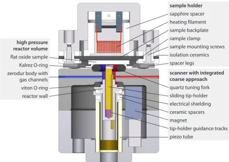
2.3.3 High pressure reactor with AFM scanner

Figure 2.1 shows the design of the AFM scanner in the high-pressure reactor cell. The model catalyst sample (typically 10×10 mm2, thickness 250 µm to 1 mm) forms the topside of the reactor, and the AFM tip approaches it from below. A Kalrez O-ring forms a leak-tight seal between the sample and the top of the scanner and closes the reactor volume. The sample is heated from the rear by a filament. Kalrez is specified for continuous use up to 600 K, and since the O-ring is in direct contact with the sample, this determines the maximum operating temperature of the scanner.

The scanner, O-ring and sample are pressed together by inflating a bellows with pressurised air. Three spacers limit the compression of the O-ring and define the mechanical loop of the scanner, resulting in a very stiff and compact design.

(32)

sample holder sapphire spacer heating filament sample backplate sample clamp sample mounting screws isolation ceramics spacer legs

scanner with integrated coarse approach quartz tuning fork sliding tip-holder electrical shielding ceramic spacers magnet

tip-holder guidance tracks piezo tube

high pressure reactor volume flat oxide sample Kalrez O-ring zerodur body with

gas channels viton O-ring reactor wall

Figure 2.1. _{The AFM version of the scanner/reactor. The Quartz Tuning Fork (QTF) is}

mounted on a magnetic rod that can slide up and down inside the piezo tube. The sliding rod rests on two tracks and is held in place by a magnet. The small high-pressure reaction cell is defined by the sample surface, two polymer O-rings, the reactor body with gas channels, and the holder for the sliding rod and tracks. The piezo tube and the sample heating filament are outside the reactor volume and remain in UHV.

1mm

(33)

of approximately 2 µm and vertical range of 1 µm. The piezo tube is located outside the high-pressure cell to avoid convective heating via the gas phase, which would result in chaotic thermal drift when operating at high temperatures.

The QTF with the AFM tip is mounted on a rod that is magnetically clamped inside the piezo tube. The rod can slide up and down during coarse approach using a stick-slip motion. The rod consists of two halves, and is held against two tracks by a Sm2Co17magnet located next to the piezo tube. Both the slider and the tracks are

made of machine steel and are gold-coated. With this coating, the static friction between the slider and tracks is sufficient to ensure that the slider does not move during normal scanning motion, but low enough to allow the stick-slip motion during coarse approach.

The tracks supporting the slider are mounted on a capped cylinder made of polyetherimide (PEI), which is located in the piezo tube. An additional cylinder made of aluminium between the PEI component and the piezo tube provides elec-trical shielding from the high piezo voltages. The PEI cylinder also forms part of the reactor wall, so the piezotube is not exposed to the high-pressure gases to avoid chemical and thermal stability issues.

The two tracks are also used as feedthroughs for the two electrical signals of the QTF through the PEI reactor wall. Each track is in contact with one of the two halves of the slider. The tracks traverse the (insulating) PEI component and are connected by coaxial cables to floating-shield BNC feedthroughs on the UHV flange of the scanner.

2.3.4 Tuning fork and tip

The quartz tuning fork is a commercial miniature crystal with a resonance frequency of 32.768 kHz, type number CM8V-T1A from Micro Crystal AG, that has been shortened by wafer cutting such that the prong length is reduced from 1.6 mm to 1.15 mm without altering its electrode topology. After modification, the overall dimensions of the tuning fork are 1.9×0.5×0.12 mm3and the fundamental resonance frequency is about 96 kHz.

The tuning fork is mounted using Stycast 2850 epoxy (with catalyst 24 LV) on the slider in the QPlus configuration[32], i.e. the lower prong is completely fixed in glue and the upper prong acts as a single piezoelectric cantilever. After gluing, the

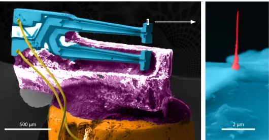
Q-factor of the first resonance at ambient conditions is 3⋅103. A ceramic (Macor[35]) spacer is used to tilt the tuning fork to an angle of 2.5○to ensure that the apex of the upper prong is the first part to come in contact with the sample surface. The resulting assembly is shown schematically in figure 2.2, and in figure 2.3.

(34)

500 μm 2 μm

Figure 2.3.Scanning Electron Microscopy images with false colours for enhanced contrast of the QTF glued on a ceramic spacer which is glued to the slider, with a close-up of the apex of the upper prong. The tip is grown using electron-beam-induced deposition of platinum from a MeCpPtMe₃precursor[34].

Nova NanoSEM 200 with MeCpPtMe₃as precursor[34], resulting in a structure consisting of 16 atom% platinum, the remainder being amorphous carbon[36]. Typical growth parameters are 15 keV electron energy, beam current of 1.4 nA, beam focused to a single spot of 5 nm, pressure 3⋅10−5mbar, for 2-5 minutes. This results in a tip with a length of 2-5 µm and a diameter of 0.1 µm. The radius of curvature of the tip apex is 30 nm. The tip is positioned on one of the electrodes of the tuning fork, but the conductivity is too low to measure tunneling currents. The tip is mechanically stiff enough for AFM measurements, but it can easily be wiped off with a tissue and replaced with a new one if needed.

The electrical connections from the tuning fork electrodes to the slider are made by ball bonding using 25 µm diameter gold wires. The electrical path contin-ues via the tracks that support the slider, followed by coaxial cables to the UHV feedthroughs.

2.3.5 Electronics

(35)

coefficient of the mechanical oscillator and this results in a shift of the resonance frequency. In the case of dissipative forces, there is also a decrease of the amplitude and an additional phase shift. The resonance frequency is measured using a phase-locked loop. The output signal of the phase-phase-locked loop is used as the input for the height feedback loop of the AFM scanner in order to trace the surface at constant frequency shift. A separate feedback system adjusts the drive amplitude to keep the oscillation amplitude constant, thereby ensuring that the surface of constant frequency shift corresponds to a surface of constant force gradient. The drive signal of this amplitude feedback loop is recorded in a separate channel and can be used to derive the dissipative force.

The tuning fork motion is controlled via an excitation/detection circuit located directly outside the UHV system. It is based on a circuit introduced by Grober et al.[38], which compensates for the stray capacitance of the tuning fork, and measures the (oscillating) current through the tuning fork with an I-V convertor when it is driven at resonance by an external oscillator voltage source. The I-V converter is based on the OPA657 operation amplifier from Texas Instruments and has a gain of 1 V/nA and a bandwidth of 100 kHz.

A Zurich Instruments HF2LI lockin amplifier with phase-locked loop detects the shift in resonance frequency of the QTF and supplies the oscillating drive voltage at resonance. The height feedback and scanning is performed using high speed SPM electronics from Leiden Probe Microscopy[39].

2.4 Performance

2.4.1 Imaging

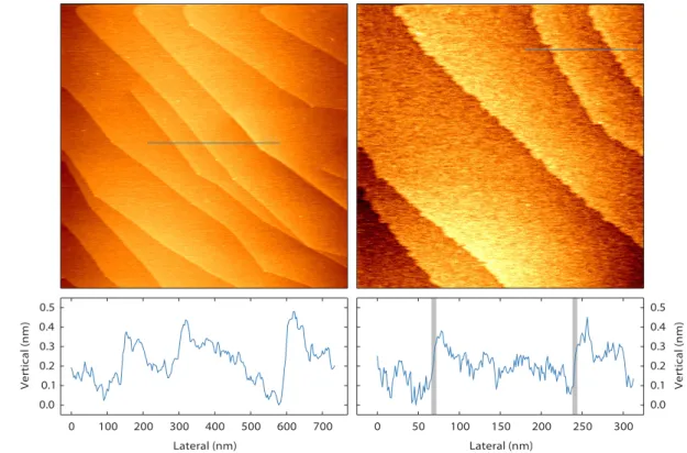
Due to limitations of the SPM control electronics it was not possible to systemati-cally characterise the performance of theReactorAFMusing force-distance curves. Instead, monoatomic terraces and steps on the (111) surface of a silver crystal have been imaged, in UHV and in flows of ethylene (figure 2.4). These images show a lateral resolution of 5 nm and a vertical resolution of 0.05 nm, as determined from the line profiles. The lateral resolution is presumably limited by the sharpness of the EBID tip.

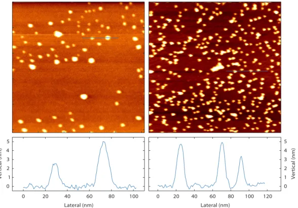
A catalytically more relevant demonstration is the imaging of palladium nanopar-ticles on a single crystal ofα−Al2O3. Figures 2.5 and 2.6 show these particles at

(36)

0 100 200 300 400 500 600 700 Lateral (nm)

0.0 0.1 0.2 0.3 0.4 0.5

Vertical (nm)

0 50 100 150 200 250 300 Lateral (nm)

0.0 0.1 0.2 0.3 0.4 0.5

Vertical (nm)

(37)

0 20 40 60 80 100 120 Lateral (nm)

0 1 2 3 4 5

Vertical (nm)

0 20 40 60 80 100 Lateral (nm)

0 1 2 3 4 5

Vertical (nm)

Figure 2.5. Palladium nanoparticles onα−Al₂O₃, image size 700×700 nm2, frequency shift setpoint +5 Hz, oscillation amplitude 5 nm, acquisition time 131 s per frame. No post processing has been performed except for planar background subtraction. Left panels, 425 K, 1 bar 1:1:20 Ar:CO:O₂mixture, total flow 5.5 mln/min. Right panels, 475 K, 1 bar 10:1:30 Ar:CO:O₂mixture, total flow 4.1 mln/min.

(38)

problem with AFM[41] — these images directly give unique information on the particle morphology and size distribution under catalytic conditions.

2.4.2 Influence of environment on QTF

Quartz resonators can be employed to measure temperature and several fluid prop-erties (density, viscosity and derived quantities)[42, 43]. These sensor applications use the resonance frequency or the damping of the oscillator to detect changes in the environment. Unfortunately, the same parameters are used to perform the height feedback in a NC-AFM configuration. Since the “parasitic” influences of the environment can be dominant over the effects “of interest” of the tip-sample interaction, a brief discussion is in place on the influence of the gas environment and the temperature.

The density and viscosity of the surrounding fluid influence the damping of the QTF, but this is easily compensated for by the amplitude feedback, and at highQ

it only results in a small change in resonance frequency. More problematic is that the fluid adds to the effective mass of the resonator[43], thereby further affecting the resonance frequency. For theReactorAFM, filling the reactor with 1000 mbar argon starting from low vacuum (<10 mbar) leads to a frequency shift of -50 Hz and a drop in Q-factor from 1⋅104to 3⋅103.

When using mixtures of gases such as oxygen, carbon monoxide, nitric oxide, carbon dioxide, nitrogen and argon, only limited total pressure variations can be tolerated because of these gas effects on resonance frequency and damping, but partial pressures can be changed freely since the fluid properties of these gases are sufficiently similar. However, when using mixtures of light gases such as hydrogen or helium together with a heavy gas, care needs to be taken not to change the total density and viscosity too much while scanning. This can be achieved by adjusting the total pressure or by compensation of the mixture by adding an appropriate amount of a heavy inert gas such as argon or xenon. In addition, the resonance frequency of the QTF is sensitive to temperature. This derives from the anisotropic thermal expansion of the crystal lattice. Since our particular QTF is designed as a reference oscillator and not as a temperature sensor, the orientation of the lattice is optimised for frequency stability at its standard operating temperature, 25○C. However, in the

(39)

A further complication can be introduced by combined effects of the fluid prop-erties with temperature: changing the gas mixture changes the thermal conductivity of the gas in the reactor and this results in a change of temperature of the QTF. Additionally, the viscosity of a fluid is strongly dependent on temperature, and this in turn influences the damping. These effects however are minimised using the precautions mentioned here.

2.5 Conclusion and outlook

TheReactorAFMcombines a UHV system with a high-pressure reactor and allows in-situ investigations of model catalysts. The scanner uses a miniature quartz tuning fork with a micrometre-sized tip, operates in non-contact mode and fits in the 0.5 ml reactor. Nanometre resolution is demonstrated under temperature, high-pressure conditions on a sample of supported metal nanoparticles. This instrument establishes an essential step to bridge thepressure gapandmaterials gap.

(40)

(41)

(42)

Chapter 3

Spacetime

: analysis software for

microscopy data of dynamical

processes

With the continuing advancement of imaging techniques along the whole spectrum of photon-, electron-, ion- and scanning probe microscopes, it has become increas-ingly common to apply such techniques for real-time,in-situstudies of dynamical systems. When analysing data from such experiments it is essential to correlate the images to parameters that have been changing during the experiment, either spontaneously or intentionally. Spacetimeis open source software to aid in this analysis by providing a single, unified view on heterogeneous datasets fromin-situ

(43)

3.1 Introduction

Some 400 years after the invention of the first microscope[44], the field of mi-croscopy is still expanding and evolving. A recent development is the application of (sub)nanometre-resolution electron- and scanning probe microscopes forin-situ

investigations of dynamical systems, that used to be limited to static ex-situ mi-croscopy investigations or macroscopic measurements on large ensembles. These microscopy studies usually involve one or more global parameters that are varied or measured while the microscope is used to image a very small, local region of the specimen, in order to unravel structure-function relationships.

Examples are catalytic studies using a scanning tunneling microscope (STM) and atomic force microscopy (AFM) inside a flow reactor[11, 45, 46], or using micromachined nanoreactors in transmission electron microscopy (TEM)[23] or scanning X-ray microscopy[47]. In the field of materials science,in-situTEM studies have been published on the hydrogenation of palladium[48] and electromigration in platinum electrodes[49]. In addition there are electrochemistry studies involving STM during deposition[50, 51].

The power of these studies lies in the correlation of the spatial microscopy data with the external parameters that either influence the system or are influenced by it. In a typical laboratory environment these external parameters are recorded from a variety of sources by specialised hardware or software. With the increas-ing complexity of such experiments, it becomes a non-trivial task to present this heterogeneous dataset, consisting of several different data types and file formats, together for analysis. For this purpose, dedicated software has been developed calledSpacetime.

3.2 Features

Spacetime aims to give a unified view on the spatial microscopy data together with any time-dependent parameter related to the dynamics of the system under investigation. It supports highly heterogeneous datasets, both in character (e.g. spatial data acquired in a single shot, spatial data acquired by a scanning technique, or purely time-dependent data) and in data format (ranging from standard image formats and plain text files to several vendor-specific formats or extensions). The emphasis is on browsing through datasets and searching for correlations to identify which subsets need to be analyzed using conventional image- or data analysis software. If desired,Spacetimeexports the originally heterogeneous dataset into a simple homogeneous format for analysis with other tools.

(44)

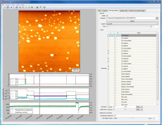
Figure 3.1._An_in-situ_{Transmission Electron Microscopy (TEM) experiment with}

(45)

them by selecting the data files and possibly defining other settings. Each module has a specific way of presenting its data. Time-dependent quantities can be plotted in graphs, showing the values versus time, while microscopy images are displayed together with a marker indicating the acquisition time and duration. The modules share a single time axis, which can be presented as an absolute date and time, or in the form of the time relative to a user-defined time origin. If needed, the timing of individual modules can be adjusted to correct for improperly synchronised clocks or propagation delays of a physical observable. The precision of the time axis is as good as 10 µs, even though many data formats have a time resolution of only 1 s.

Combined data can be exported to various raster and vector image formats, and can be animated and saved as a movie. For presentation purposesSpacetime

features a split-screen presentation mode, where the projector shows the selected combination of experimental data while the control interface remains on the com-puter/laptop screen.

3.3 Implementation

Spacetimehas been written in Python, a general-purpose programming language that is becoming increasingly popular in the scientific community[52].Spacetime

uses various open-source libraries, including NumPy[53] (numerical computation), Matplotlib[54] (plotting) and the Enthought TraitsUI toolkit[55] (graphical user interface or GUI). This makesSpacetimefully platform-independent so that it runs on e.g. Windows, Linux and Mac OS X.

The code is modular and easily extensible. The description of the GUI, the plotting logic and the data handling code is fully separated for each of the supported file formats. This means that when adding a new file format, only the actual file handling code has to be written, the plotting code, and GUI can be reused from other modules. Similarly, there can be multiple different graph types for a single file format.

At the time of this writing, the following file formats are supported: basic image formats (including PNG, JPEG, TIFF and BMP), basic plain text formats (CSV and tabulated), Leiden Probe Microscopy[56] Camera RAW files for scanning probe mi-croscopy, Gatan DigitalMicrograph 3[57] (DM3) images and stacks for transmission electron microscopy, TVIPS[58] extensions for TIFF images for transmission elec-tron microscopy, and various mass spectrometer formats from Pfeiffer Vacuum[59], Stanford Research Systems[60] and MKS Instruments[61].

(46)

Figure 3.2._{Another screenshot from}_Spacetime_{: Pd nanoparticles on}_α_-Al₂_O₃_{during an}

(47)

3.4 Outlook

Spacetimeis a flexible tool for exploring the heterogeneous datasets typically ac-quired during microscopy studies of dynamical processes, but can be used with any dataset combining two-dimensional images with time-dependent data. Future plans include arbitrary transformations of the time-axis using mathematical expres-sions or measurement data and expanding the number of supported file formats.

(48)

(49)

(50)

Chapter 4

BINoculars

: data reduction and

analysis software for

two-dimensional detectors in

surface X-ray diffraction

BINocularsis a tool for data reduction and analysis of large sets of surface diffraction data that have been acquired with a 2D X-ray detector. The intensity of each pixel of a 2D-detector is projected onto a 3-dimensional grid in reciprocal lattice coordinates using a binning algorithm. This allows for fast acquisition and processing of high-resolution datasets and results in a significant reduction of the size of the dataset. The subsequent analysis then proceeds in reciprocal space. It has evolved from the specific needs of the ID03 beamline at the ESRF, but it has a modular design and can be easily adjusted and extended to work with data from other beamlines or from other measurement techniques. This chapter covers the design and the underlying methods employed in this software package and explains howBINoculars

can be used to improve the workflow of surface X-ray diffraction measurements and analysis.

(51)

4.1 Introduction

Over the last decade there have been several developments that have radically changed data acquisition in X-Ray Diffraction (XRD) experiments. The primary development is that nearly all point detectors have been replaced by 2D-detectors, such as the MAXIPIX detector[64], that collect spatially resolved information from a region in reciprocal space in a single shot. Secondly, by synchronising the data acquisition with the actuation of the diffractometer motors, it is now possible to perform continuous scans during diffractometer movements. Even though this has been demonstrated already 50 years ago[65], it has only recently become routine practice[66]. Thirdly, the high photon flux at 3rd generation synchrotrons[67] allows integration times in the order of tens of milliseconds rather than seconds, thus enabling time-dependent observations of dynamic processes rather than the slow acquisition of static information.

The result of these developments is that the data acquisition rate has increased by six to seven orders of magnitude, from typically 1 point per second to millions of points per second, so the amount of data collected during one experiment increased dramatically. Today’s computer hardware can keep up with that increased demand, but the development of software to analyze these large datasets has been lagging behind, which has kept most users from exploiting the full potential of modern surface diffraction beamlines. BINocularsaims to fill this gap by taking a novel approach to data reduction in Surface X-Ray Diffraction (SXRD) experiments.

Currently, data reduction is typically performed by integrating a region of the image from a 2D-detector, sometimes coupled with another integration to determine the background level, and then basically treating the data as if it would have come from a point detector. Compared to a traditional point detector the advantages are mostly qualitative: the large acceptance angle of the detector, in combination with its good angular resolution, is very convenient during diffractometer and sample alignment, and makes it possible to visually identify peaks by their shape (i.e. one can easily distinguish between a powder ring, a crystal truncation rod or a region of diffuse background).BINocularsimproves on this by treating every pixel of a 2D-detector individually, rather than to reduce the 2D-detector to an expensive point detector.

BINocularstakes a series of images from a 2D-detector, calculates for each pixel the corresponding reciprocal lattice coordinates(h k l), and reduces the image collection to a single dataset by averaging the intensities of pixels taken at identical

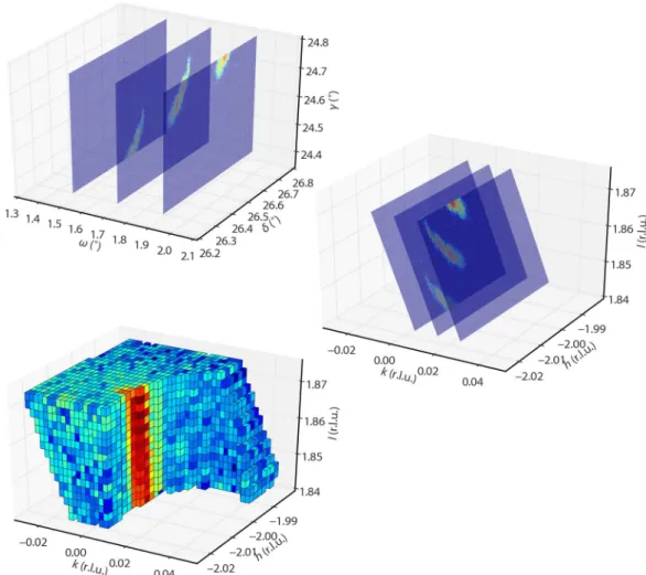
(h k l)positions (within a user-specified resolution). This transformation and aver-aging is illustrated in figure 4.1. To allow online analysis during data acquisition,

(52)

Figure 4.1.A graphical overview of the process performed byBINoculars. The data displayed here are a rocking scan through(h,k,l) = (−2, 0, 1.85)the diffraction pattern from a Pt(110) surface. Upper panel, raw data acquired by the 2D-detector with the corresponding angles

(53)

BINocularsprovides tools to further process the data, including visualisation, curve fitting, and crystal truncation rod integration. The latter can be seen as an imple-mentation of the reciprocal-space integration method, recently described by Drnec et al[69]. As a whole,BINocularscan be seen as a N-dimensional generalisation of PyFAI[70] and xrayutilities[71], optimised for (but not limited to) surface X-ray diffraction.

4.2 Implementation

BINocularshas been written in Python, an open source scripting language that is very suitable for scientific software, thanks to its powerful and clear syntax and the extensive support for numerical calculations via the Numpy and Scipy libraries[52].

BINocularshas been designed to process large datasets, and its operation is usually cpu-bound. An ordinary desktop computer can easily take many hours to deal with a dataset obtained in one hour (e.g. 1010pixels with 16 bit per pixel). To allow online analysis during data acquisition at a beamline,BINocularscan use a computing cluster to distribute the load over multiple computers.

To keepBINocularsmodular and flexible, the workflow for processing data is separated into four modules: thedispatcheris in charge of the whole process and handles job parallelization and distribution, theinputclass gathers the experimental data, and theprojectionclass converts the raw data into the coordinates of choice. Finally, the processed data is binned on a discrete grid and stored in aspaceclass, which provides generic tools for further analysis. The specific behaviour of the

dispatcher,inputandprojectionmodules can be changed independently. For these modules, the user can choose from several different implementations, each having a different set of features.

Theinputclass collects the raw 2D-detector images and assigns metadata to each individual pixel. This metadata is used later on by theprojectionclass to make the conversion to the desired coordinate system (e.g.(h k l)for a typical SXRD experiment). Theinputclass is specific to a certain experimental setup. As an example, for the ID03 beamline at the ESRF[72], a separate class has been written for each of the experimental hutches. In many ways the two experimental hutches are identical, for example the same numbering scheme is used for the images taken by the X-ray cameras, but one of the diffractometers operates at constant detector-sample distance while the other does not. Theinputclass takes care of all these technicalities, and writing a newinputis the most important task when adding support for another experimental setup. In addition, the work done by theinputclass is often the most computationally intensive step in the entire process ofBINoculars.

(54)

intensities from all images, binned on discrete (h k l) coordinates, stored on disk in HDF5 format

space dispatcher

node 1 node 2 node n

input

projection

space

2D image annotated with diffractometer angles

2D image annotated with

(h k l) coordinates

intensities from one image, binned on discrete (h k l) coordinates

input

projection

space

input

projection

space . . .

. . . . . .

Figure 4.2. Block diagram of the process performed byBINocularsfor a typical dataset from a diffraction experiment. Thedispatcherdistributes the load over multiple nodes from a computing cluster. Theinputclass gathers the experimental data and calculates the diffractometer angles for each pixel. Theprojectionclass converts the angles to(h k l)

(55)

an SXRD experiment, theinputclass will typically return a series of detector images with corresponding diffractometer angles for each pixel, and theprojectionclass will convert the angles into reciprocal space coordinates(h k l)for each image. In some cases, there are several projections that are useful. For example, for the ID03 beamline it is sometimes necessary to project onto the scattering angle 2θ

rather than(h k l)coordinates (although an alternative route would be to perform a coordinate transformation afterwards to convert the(h k l)spaceinto a 2θ space). Once the data has been gathered and projected on the desired coordinate system, the binning operation is performed by a class calledspace. This class represents ann-dimensional regular grid: it is a discrete subset of a vector space, where each dimension has a fixed step size. Many mathematical operations can be performed withspaces, including addition, subtraction, slicing, projections, and coordinate transformations. To bin an image, the(h k l)coordinates of each pixel of the image are mapped onto the nearest discretespacegrid location. Then the pixel intensities are accumulated at every discrete grid location, using the histogram-operation

bincountfrom Numpy. In addition, the number of contributions per coordinate is stored in order to calculate the mean intensity per bin rather than the integrated intensity. This binning operation is the essential data reduction step performed by

BINoculars, hence the name of the program.

Thedispatcherorchestrates the entire process: it asksinputfor the sequence of images from the 2D-detector, delegates it to the appropriateprojectionand performs the binning operation by feeding the projection result into aspace. Twodispatcher

implementations are currently present: one for local processing using multiple processor cores on a single computer, and one that distributes tasks over a high performance cluster managed using OAR[73]. Support for other types of clusters can easily be added. When running on a computing cluster, thedispatchergathers all intermediate spaces calculated by the individual nodes (for example using a shared filesystem) and they are added together to form the final resultingspace.

Spacesare stored on disk using the HDF5 file format[74].

After aspacehas been created, the size of the dataset has typically been reduced by a factor 10 to 100, and further analysis can usually be performed on a standard workstation. However, loading a high-resolution large-area 3D dataset can require several GB of memory, and for some operations it is required to have several copies in memory. If this is a problem, it is also possible to work with a subset of the data, either by selecting a smaller region, or by reducing the resolution, or by reducing the dimensionality.

(56)

the structure factors of a crystal truncation rod to be directly inserted into the fitting program ROD[75]. It takes as input a reciprocal mesh which it slices by a user-specified resolution and the resulting data are either fitted (typically with a 2D lorentzian) using a least-squares optimization, or simply integrated. The error is estimated from equation (4.2), as will be described in more detail in the next section.

4.3 Binning and error handling

BINocularscalculates the average intensity of multiple contributions, originating from different pixels and/or detector positions, to a single reciprocal space bin. This operation is similar but not identical to averaging a series of repeated measurements taken by a point detector at a fixed position. This section discusses the implications of the binning operation for the background intensity and the estimation of statistical errors.

When using a point detector, the typical surface diffraction experiment is set up such that there is a unique detector position for each set of reciprocal space coordinates(h k l). In practice, this means reducing the degrees of freedom of the diffractometer to three, e.g. by working with a constant surface normal and a fixed angle of incidence. When taking series of repeated observations at a certain reciprocal-space location, the systematic error in each measurement can be assumed to be constant (after the usual correction for variations in the total beam intensity), and the only variation is given by the shot noise of the incoming photons.

Using a 2D-detector, the spatial extent of the detector introduces two more degrees of freedom, meaning there is no longer a unique detector position for a given reciprocal space coordinate. This is usually solved by selecting one pixel of the detector to correspond with “the detector position”, and ignoring the fact that the other pixels are at a slightly different position. However,BINocularsdoes take the spatial extent of the detector into account, and calculates the average intensity at each location in reciprocal space, regardless of the detector position.

This means that multiple measurements, even when spaced closely together in time, exhibit variations not only due to the statistical nature of the process, but also due to a systematic error possibly resulting from different detector positions. This error is caused by differences in background originating from scatterers other than the sample, as is illustrated in figure 4.3. Flight tubes and slits between the sample and the detector can be used to reduce this background, but they also decrease the aperture of the 2D-detector. This reduces the range of(h k l)-locations over which data can be collected in one acquisition. This means that a careful trade-off needs to be made between acquisition speed and background suppression.

(57)

2D detector

slits

sample window

incoming x-rays

diffr acted x

-rays

Figure 4.3. The wide opening angle of the slits, which is required to capture a region in reciprocal space with a 2D-detector, results in a non-uniform background across the detector (indicated in grey in the figure). This background originates from scatterers other than the sample, for example a beryllium window. This means that when taking two images at slightly different detector positions such that there is some overlap between the two captured regions, the background intensity in the overlapping region is not constant.

it directly when the sample is not in the beam, or by estimating it from the dataset itself in regions in reciprocal space where the sample only weakly contributes to the total observed intensity. The latter approach will be explored in more detail in section 4.4.

The remaining error reflects the counting statistics in the number of detected photons and is typically assumed to obey Poisson statistics[76]. For a single obser-vation ofIcounts, the standard deviationσ is estimated usingσ =√I. WithN

independent observationsIi in a single bin, each with its ownσi =

√

Ii, the average

intensity is

I= 1

N ∑_i Ii, (4.1)

and the variance can be estimated under the assumption of normality (N orIi

sufficiently large) using

σ2≈ 1 N2(∑i

σi2) =

I

N. (4.2)

Assuming we have a separate estimate of the background intensityIbin this bin

with a corresponding varianceσ_b2, the the varianceσs2of the signalIs=I−Ibis now

given by

σs2=I/N+σb2. (4.3)

Of course, if the background was also obtained by averagingNmeasurements,

(58)

4.4 Demonstration

Four different examples will be discussed to show the capabilities and limitations of

BINoculars.

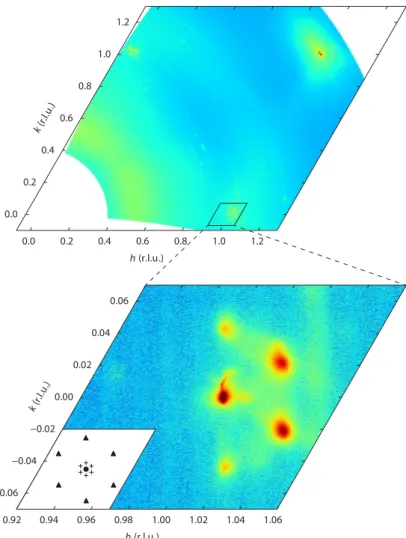
Figure 4.4 shows a high-resolution (0.0002 reciprocal lattice units or r.l.u.), large-area(hk)-surface in reciprocal space, covering the first reciprocal unit cell of a Au(111) surface, submerged in an electrochemical cell filled with sulphate containing electrolyte (pH 7) and kept at -800 mV vs. Ag/AgCl reference electrode. The gold surface exhibited the so-called herringbone reconstruction[77], which is a regular structure with a (22×√3 periodicity) that is organised into a zigzag pattern on an even larger scale. The(22×√3)superstructure peaks originating from this reconstruction[78, 79] are well-resolved in the scan. The differences between this diffraction pattern and the pattern reported in literature for the same surface in ultrahigh vacuum are not fully understood, however it is likely due to the sample preparation procedure in the electrochemical cell. The dataset was acquired in just 111 minutes.

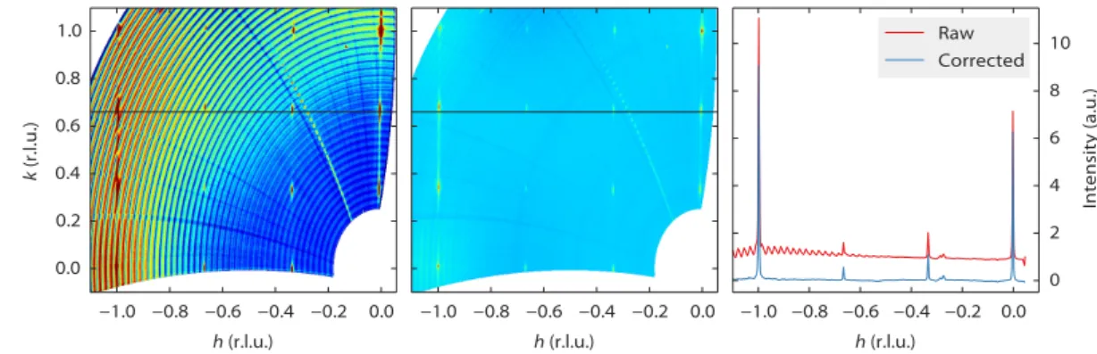
Figure 4.5 shows a dataset that is strongly affected by background intensity. Like figure 4.4, the dataset is built up from a series ofω-scans and in this case those scans are clearly visible as arcs after processing byBINoculars. The problem is that the background intensity not only depends on the position of a pixel, but also on the position of the camera. In other words, when moving the camera by only a small amount, such that a certain feature remains in the field of view (in this case a move inγbetween the consecutiveω-arcs), the contribution of the background intensity to that feature can change significantly, as illustrated in figure 4.3.

This particular dataset has been obtained using the high-pressure flow reactor setup at ID03[22], which has a beryllium dome around the sample. The dome acts as a strong X-ray scatterer only 14 mm away from the sample. It is not possible to lower the resulting background intensity using slits without dramatically reducing the aperture of the detector. However, for this sample it proved possible to estimate and subtract the background level, the result of which is shown in the middle panel of figure 4.5. For each pixel of the detector, the background was estimated as the average intensity of that pixel in all images in a singleω-scan. The average is calculated by fitting a Poisson distribution, as this turned out to give better rejection of outliers (which are in fact the diffraction peaks) than a simple mean or median calculation. This process was then repeated for eachω-scan, resulting in an estimate of the background intensity that was subtracted from the raw data.

(59)

0.0 0.2 0.4 0.6 0.8 1.0 1.2

h (r.l.u.) 0.0

0.2 0.4

0.6 0.8

1.0 1.2

k (r .l.u.

)

0.92 0.94 0.96 0.98 1.00 1.02 1.04 1.06

h (r.l.u.) −0.06

−0.04 −0.02

0.00 0.02

0.04 0.06

k (r.l. u.)

Figure 4.4. _{A large-area survey (upper panel) in reciprocal space of the herringbone}

reconstructed Au(111) surface, taken atl=0.3. The dataset has been obtained in 111 minutes using a series of continuous-acquisitionω-scans. A zoom-in (lower panel) around the

(60)

−1.0 −0.8 −0.6 −0.4 −0.2 0.0

h (r.l.u.) 0.0 0.2 0.4 0.6 0.8 1.0 k ( r. l.u .)

−1.0 −0.8 −0.6 −0.4 −0.2 0.0

h (r.l.u.)

−1.0 −0.8 −0.6 −0.4 −0.2 0.0

h (r.l.u.)

0 2 4 6 8 10 Intensity (a.u.) Raw Corrected

Figure 4.5.Some datasets require further processing to remove the curved background artefacts. This figure shows thel=0.5 plane from a Pt(110) sample in the high-pressure flow reactor setup at ID03. The surface exhibited a(3×3)reconstruction (which has not been described before in literature) during high-temperature, high-pressure exposure to NO and H₂. The setup had a relatively high diffuse background that could be corrected for by estimating the background level for each pixel of the detector, once per scan inω. The left panel shows the raw data, the middle panel the data after background correction. The right panel shows the intensity profiles along the linek=0.66 for a direct comparison between raw and corrected data. The small peaks ath=0.3 originate from scattering from the Be dome, this is also visible in the left and middle panel as a diagonal line.

module in the near future.

The third example, figure 4.6, shows the output of the crystal truncation rod (CTR) fitting module. The original dataset is a singlel-scan along the CTR. After processing byBINoculars, during which theinputmodule also takes care of the polarization correction factor necessary to obtain the structure factors[68], the three-dimensional rod can be visualised in reciprocal space. The dataset is then segmented into small intervals alongl. Each section is analysed separately by a numerical integration algorithm to calculate the structure factors as a function ofl. This method has recently been described by Drnec and co-workers[69].

At lowerlthe detector is more perpendicular to the surface, and for some sam-ples it might be useful to augment thel-scan with rocking scans at lowl.BINoculars

can easily deal with such a hybrid dataset, since it starts by processing the data into the three-dimensional rod, after which the integration procedure (taking place in reciprocal space) is performed completely independently of the original character of the raw data.

The fourth example demonstrates that BINoculars can be used with other coordinate systems than (h k l). Figure 4.7 shows the reflected intensity from a (PbSe)₄₊_δ(TiSe₂)₄ sample. It is constructed from images taken at different in-cidence angles that are projected ontoq∥andqz, the in-plane and out-of-plane

The structure of a working catalyst : from flat surfaces to nanoparticles

Cover Page

The handle

http://hdl.handle.net/1887/29891

holds various files of this Leiden University

dissertation

Author

: Roobol, Sander Bas

Title

: The structure of a working catalyst : from flat surfaces to nanoparticles

The structure of a working catalyst

From flat surfaces to nanoparticles

The structure of a working catalyst

The structure of a working catalyst

From flat surfaces to nanoparticles

About this thesis

Contents

Chapter 1

Introduction

The pressure gap and the materials gap

New instrumentation to bridge the gaps

Operando catalysis

A multi-technique approach

Part I

Chapter 2

The

ReactorAFM

: Non-Contact

Atomic Force Microscope

operating under high-pressure

and high-temperature catalytic

conditions

2.1 Introduction

2.2 Design specifications

2.3 Design

2.4 Performance

2.5 Conclusion and outlook

Chapter 3

Spacetime

: analysis software for

microscopy data of dynamical

processes

3.1 Introduction

3.2 Features

3.3 Implementation

3.4 Outlook

Chapter 4

BINoculars

: data reduction and

analysis software for

two-dimensional detectors in

surface X-ray diffraction

4.1 Introduction

4.2 Implementation

4.3 Binning and error handling

4.4 Demonstration