K2 Observations of SN 2018oh Reveal a Two Component Rising Light Curve for a Type Ia Supernova

(1)

K2 Observations of SN 2018oh Reveal a Two-Component Rising Light Curve for a Type Ia Supernova G. Dimitriadis,1 R. J. Foley,1 A. Rest,2, 3 D. Kasen,4, 5 A. L. Piro,6 A. Polin,7, 8 D. O. Jones,1 A. Villar,9 G. Narayan,3 D. A. Coulter,1 C. D. Kilpatrick,1 Y. -C. Pan,1 C. Rojas-Bravo,1 O. D. Fox,2 S. W. Jha,10

P. E. Nugent,7, 8 A. G. Riess,2, 3 D. Scolnic,11and M. R. Drout6,∗ —

K2 Mission Team

G. Barentsen,12, 13 J. Dotson,12M. Gully-Santiago,12, 13 C. Hedges,12, 13 A. M. Cody,12, 13 T. Barclay,14, 15 and S. Howell12

— KEGS

P. Garnavich,16 B. E. Tucker,17, 18, 19 E. Shaya,20 R. Mushotzky,20 R. P. Olling,20 S. Margheim,21 and A. Zenteno22

—

Kepler spacecraft team

J. Coughlin,12, 23 J. E. Van Cleve,12, 23 J. Vin´ıcius de Miranda Cardoso,12, 24 K. A. Larson,25 K. M. McCalmont-Everton,25C. A. Peterson,25 S. E. Ross,25 L. H. Reedy,26 D. Osborne,26C. McGinn,26

L. Kohnert,26 L. Migliorini,26 A. Wheaton,26 B. Spencer,26C. Labonde,26G. Castillo,26 G. Beerman,26 K. Steward,26 M. Hanley,26 R. Larsen,26 R. Gangopadhyay,26R. Kloetzel,26 T. Weschler,26 V. Nystrom,26 J. Moffatt,26 M. Redick,26 K. Griest,26 M. Packard,26 M. Muszynski,26 J. Kampmeier,26 R. Bjella,26 S. Flynn,26

and B. Elsaesser26 —

Pan-STARRS

K. C. Chambers,27 H. A. Flewelling,27 M. E. Huber,27E. A. Magnier,27 C. Z. Waters,27 A. S. B. Schultz,27 J. Bulger,27 T. B. Lowe,27 M. Willman,27 S. J. Smartt,28 and K. W. Smith28

— DECam

S. Points22 and G. M. Strampelli2, 29 —

ASAS-SN

J. Brimacombe,30P. Chen,31 J. A. Mu˜noz,32, 33 R. L. Mutel,34 J. Shields,35P. J. Vallely,35and S. Villanueva Jr.35 —

PTSS/TNTS

W. Li,36, 37 X. Wang,36J. Zhang,38, 39, 40 H. Lin,36J. Mo,36X. Zhao,41H. Sai,36X. Zhang,36 K. Zhang,36, 42 T. Zhang,43 L. Wang,43, 44 J. Zhang,36 E. Baron,45 J. M. DerKacy,45 L. Li,36Z. Chen,36D. Xiang,36 L. Rui,36

L. Wang,46, 47 F. Huang,48, 36 and X. Li36 —

Las Cumbres Observatory

G. Hosseinzadeh,37, 49 D. A. Howell,37, 49 I. Arcavi,37, 49, 50,† D. Hiramatsu,37, 49 J. Burke,37, 49 and S. Valenti51 —

ATLAS

J. L. Tonry,27L. Denneau,27 A. N. Heinze,27 H. Weiland,27 and B. Stalder52 —

Konkoly

J. Vinkó,53, 54, 42 K. Sárneczky,53A. Pál,53 A. Bódi,53, 55 Zs. Bognár,53 B. Csák,53 B. Cseh,53G. Csörnyei,53 O. Hanyecz,53 B. Ignácz,53Cs. Kalup,53 R. Könyves-Tóth,53 L. Kriskovics,53 A. Ordasi,53 I. Rajmon,56

A. Sódor,53 R. Szabó,53 R. Szakáts,53 and G. Zsidi53 —

ePESSTO

S. C. Williams,57 J. Nordin,58 R. Cartier,22 C. Frohmaier,59 L. Galbany,60 C. P. Guti´errez,61 I. Hook,57 C. Inserra,61and M. Smith61

—

University of Arizona

Corresponding author: Georgios Dimitriadis [email protected]

(2)

D. J. Sand,62 J. E. Andrews,62 N. Smith,62 and C. Bilinski62

1_{Department of Astronomy and Astrophysics, University of California, Santa Cruz, CA 95064, USA} 2_{Space Telescope Science Institute, 3700 San Martin Drive, Baltimore, MD 21218, USA} 3_{Department of Physics and Astronomy, Johns Hopkins University, Baltimore, MD 21218, USA}

4_{Department of Astronomy, University of California, Berkeley, CA 94720-3411, USA} 5_{Lawrence Berkeley National Laboratory, 1 Cyclotron Road, Berkeley, California 94720, USA} 6_{The Observatories of the Carnegie Institution for Science, 813 Santa Barbara St., Pasadena, CA 91101, USA}

7_{Department of Astronomy, University of California, Berkeley, CA, 94720-3411, USA} 8_{Lawrence Berkeley National Laboratory, Berkeley, CA, 94720, USA}

9_{Harvard-Smithsonian Center for Astrophysics, 60 Garden Street, Cambridge, MA 02138, USA}

10_{Department of Physics and Astronomy, Rutgers, The State University of New Jersey, 136 Frelinghuysen Road, Piscataway, NJ 08854,}

USA

11_{Kavli Institute for Cosmological Physics, University of Chicago, Chicago, IL 60637, USA} 12_{NASA Ames Research Center, Moffett Field, CA 94035, USA}

13_{Bay Area Environmental Research Institute, P.O. Box 25, Moffett Field, CA 94035, USA} 14_{NASA Goddard Space Flight Center, 8800 Greenbelt Rd, Greenbelt, MD 20771, USA} 15_{University of Maryland, Baltimore County, 1000 Hilltop Cir, Baltimore, MD 21250, USA}

16_{Department of Physics, University of Notre Dame, 225 Nieuwland Science Hall, Notre Dame, IN, 46556-5670, USA} 17_{The Research School of Astronomy and Astrophysics, Mount Stromlo Observatory, Australian National University, Canberra, ACT}

2611, Australia

18_{National Centre for the Public Awareness of Science, Australian National University, Canberra, ACT 2611, Australia} 19_{The ARC Centre of Excellence for All-Sky Astrophysics in 3 Dimension (ASTRO 3D), Australia}

20_{Astronomy Department, University of Maryland, College Park, MD 20742-2421, USA} 21_{Gemini Observatory, La Serena, Chile}

22_{Cerro Tololo Inter-American Observatory, Casilla 603, La Serena, Chile} 23_{SETI Institute, 189 Bernardo Avenue, Mountain View, CA 94043, USA}

24_{Universidade Federal de Campina Grande, Campina Grande, Brazil} 25_{Ball Aerospace and Technologies Corp., Boulder, Colorado, 80301, USA}

26_{LASP, University of Colorado at Boulder, Boulder, CO 80303, USA}

27_{Institute of Astronomy, University of Hawaii, 2680 Wood- lawn Drive, Honolulu, Hawaii 96822, USA} 28_{Astrophysics Research Centre, School of Mathematics and Physics, Queens University Belfast, Belfast BT7 1NN, UK}

29_{University of La Laguna, Calle Padre Herrera, 38200 San Cristbal de La Laguna, Santa Cruz de Tenerife, Spain} 30_{Coral Towers Observatory, Cairns, Queensland 4870, Australia}

31_{Kavli Institute for Astronomy and Astrophysics, Peking University, Yi He Yuan Road 5, Hai Dian District, Beijing 100871, China} 32_{Departamento de Astronom´ıa y Astrof´ısica, Universidad de Valencia, E-46100 Burjassot, Valencia, Spain}

33_{Observatorio Astron´}_{omico, Universidad de Valencia, E-46980 Paterna, Valencia, Spain} 34_{Department of Physics and Astronomy, University of Iowa, Iowa City, IA 52242, USA}

35_{Department of Astronomy, The Ohio State University, 140 West 18th Avenue, Columbus, OH 43210, USA} 36_{Physics Department and Tsinghua Center for Astrophysics (THCA), Tsinghua University, Beijing, 100084, China}

37_{Las Cumbres Observatory, 6740 Cortona Dr Ste 102, Goleta, CA 93117-5575, USA} 38_{Yunnan Astronomical Observatory of China, Chinese Academy of Sciences, Kunming, 650011, China}

39_{Key Laboratory for the Structure and Evolution of Celestial Objects, Chinese Academy of Sciences, Kunming 650216, China} 40_{Center for Astronomical Mega-Science, Chinese Academy of Sciences, 20A Datun Road, Chaoyang District, Beijing, 100012, China}

41_{School of Science, Tianjin University of Technology, Tianjin, 300384, China} 42_{Department of Astronomy, University of Texas at Austin, Austin, TX, 78712, USA} 43_{National Astronomical Observatory of China, Chinese Academy of Sciences, Beijing, 100012, China}

44_{Chinese Academy of Sciences South America Center for Astronomy, China-Chile Joint Center for Astronomy, Camino El Observatorio}

1515, Las Condes, Santiago, Chile

45_{Homer L. Dodge Department of Physics and Astronomy, University of Oklahoma, Norman, OK} 46_{Purple Mountain Observatory, Chinese Academy of Sciences, Nanjing 210034, China}

47_{George P. and Cynthia Woods Mitchell Institute for Fundamental Physics}_&_{Astronomy, Texas A.}_&_{M. University, Department of}

Physics and Astronomy, 4242 TAMU, College Station, TX 77843, USA

48_{Department of Astronomy, School of Physics and Astronomy, Shanghai Jiao Tong University, Shanghai, 200240, China} 49_{Department of Physics, University of California, Santa Barbara, CA 93106-9530, USA}

50_{The Raymond and Beverly Sackler School of Physics and Astronomy, Tel Aviv University, Tel Aviv 69978, Israel} 51_{Department of Physics, University of California, 1 Shields Ave, Davis, CA 95616-5270, USA}

(3)

53_{Konkoly Observatory, MTA CSFK, Konkoly Thege M. ut 15-17, Budapest, 1121, Hungary} 54_{Department of Optics & Quantum Electronics, University of Szeged, Dom ter 9, Szeged, 6720 Hungary}

55_{MTA CSFK Lend¨}_{ulet Near-Field Cosmology Research Group} 56_{Berzsenyi D´}_{aniel High School, K´}_arp´_{at utca 49-53, Budapest, 1133, Hungary}

57_{Department of Physics, Lancaster University, Lancaster, LA1 4YB, UK}

58_{Institute of Physics, Humboldt-Universit¨}_{at zu Berlin, Newtonstr. 15, 12489 Berlin, Germany} 59_{Institute of Cosmology and Gravitation, University of Portsmouth, Portsmouth, PO1 3FX, UK} 60_{PITT PACC, Department of Physics and Astronomy, University of Pittsburgh, Pittsburgh, PA 15260, USA}

61_{Department of Physics and Astronomy, University of Southampton, Southampton, SO17 1BJ, UK} 62_{Steward Observatory, University of Arizona, 933 North Cherry Avenue, Rm. N204, Tucson, AZ 85721-0065, USA}

ABSTRACT

We present an exquisite, 30-min cadenceKepler (K2) light curve of the Type Ia supernova (SN Ia) 2018oh (ASASSN-18bt), starting weeks before explosion, covering the moment of explosion and the subsequent rise, and continuing past peak brightness. These data are supplemented by multi-color Pan-STARRS1 and CTIO 4-m DECam observations obtained within hours of explosion. The K2 light curve has an unusual two-component shape, where the flux rises with a steep linear gradient for the first few days, followed by a quadratic rise as seen for typical SNe Ia. This “flux excess” relative to canonical SN Ia behavior is confirmed in our i-band light curve, and furthermore, SN 2018oh is especially blue during the early epochs. The flux excess peaks 2.14±0.04 days after explosion, has a FWHM of 3.12±0.04 days, a blackbody temperature ofT = 17,500+11,500₋_9,000 K, a peak luminosity of 4.3±0.2×1037erg s−1, and a total integrated energy of 1.27±0.01×1043erg. We compare SN 2018oh to several models that may provide additional heating at early times, including collision with a companion and a shallow concentration of radioactive nickel. While all of these models generally reproduce the early K2 light curve shape, we slightly favor a companion interaction, at a distance of∼2×1012_cm

based on our early color measurements, although the exact distance depends on the uncertain viewing angle. Additional confirmation of a companion interaction in future modeling and observations of SN 2018oh would provide strong support for a single-degenerate progenitor system.

Keywords: supernovae: general — supernovae: individual (SN 2018oh)

1. INTRODUCTION

Through a combination of theoretical arguments and strong observational constraints, it has long been un-derstood that Type Ia supernovae (SNe Ia) are the re-sult of a thermonuclear explosion of a carbon/oxygen white dwarf (WD) (e.g., Hoyle & Fowler 1960;Colgate & McKee 1969;Woosley et al. 1986;Bloom et al. 2012) in a binary system. Nevertheless, despite SNe Ia be-ing used to discover the acceleratbe-ing expansion of the Universe two decades ago (Riess et al. 1998;Perlmutter

et al. 1999) and continuing to be a powerful dark energy

probe (e.g., Scolnic et al. 2018; Jones et al. 2018), we still do not know the nature of their progenitor systems, whether they come from multiple progenitor scenarios, and if so, in what proportion.

Roughly speaking, possible SN progenitor systems can be separated into two main classes (or channels): the single-degenerate (SD) channel, where the primary

∗_{Hubble Fellow, Dunlap Fellow}

†_{Einstein Fellow}

WD accretes material from a non-degenerate compan-ion triggering a thermonuclear runaway near the Chan-drasekhar mass (MCh) (e.g.,Whelan & Iben 1973), and

the double-degenerate (DD) channel where the SN is triggered by the merger of two WDs (e.g.; Iben &

Tu-tukov 1984). Numerical modeling of explosions (e.g.,

Hillebrandt & Niemeyer 2000; Hillebrandt et al. 2013) combined with radiative hydrodynamic modeling (e.g.,

Kasen et al. 2009;Woosley & Kasen 2011;Pakmor et al. 2012;Sim et al. 2012,2013) indicate that the basic prop-erties of the SN Ia population can be reproduced by ei-ther scenario. Therefore, we must turn to observations to further constrain the possible progenitor systems of SNe Ia.

Thus far, the observations have been similarly lim-ited, and are often inconsistent with a single scenario. No SN Ia progenitor system has yet been directly ob-served in the handful of SNe Ia with reasonably deep pre-explosion images (Li et al. 2011;Goobar et al. 2014;

Kelly et al. 2014) (although one has for a peculiar WD

(4)

progenitor systems. On a different approach, a search for the surviving non-degenerate companion star at the central regions of SN remnants (SNRs), believed to have a SN Ia origin, also excludes WD + sub-giant or red gi-ant (RG) systems (Kerzendorf et al. 2012; Schaefer &

Pagnotta 2012; Kerzendorf et al. 2014). Nonetheless,

several indirect observations can reveal the nature of the companion with some scenarios having specific and distinct observational predictions.

Observing SNe Ia as close to explosion as possible can provide unique information for distinguishing between progenitor scenarios. For example, the earliest moments can be dominated by the shock cooling of the explod-ing WD (Piro et al. 2010), which was used in the case of SN 2011fe to constrain the explosion to be coming from a degenerate star (Bloom et al. 2012). For SD progenitor systems containing a Roche-lobe-filling com-panion, signs of the SN ejecta interacting with the non-degenerate companion star are expected for some lines of sight (Kasen 2010). This produces strong X-ray and UV/optical emission that will surpass the radioactive lu-minosity of the SN at these early epochs. The amount of observed flux depends on the viewing angle and the dis-tance between the exploding WD and the companion — which given the Roche-lobe overflow assumption, pro-vides constraints on the companion star radius. Specif-ically, evolved red giants are expected to produce more flux than smaller stars.

While early excess emission is a robust prediction for the Roche-lobe-filling SD scenarios, other physical phe-nomena can possibly also produce early heating. In par-ticular,56Ni near the surface (i.e., with a mass fraction exceeding that of lower layers) should also introduce flux in excess of the canonical “expanding fireball” model

(Piro & Nakar 2013). This scenario, which can occur

for both progenitor channels, can conceal or resemble interaction models. A specific explosion model that can produce such a configuration is the double-detonation explosion of a sub-MchWD, where the detonation of a

surface helium layer will produce significant surface56_Ni

(Noebauer et al. 2017). Piro & Morozova (2016) also found that shallow56_{Ni distributions and/or interaction}

with circumstellar material (CSM) expelled during a DD merger can modulate the early light curve shape.

Observations early enough and with sufficient cadence to search for these early light curve features are still rel-atively rare. Nearby events, such as SNe 2011fe (Nugent

et al. 2011; Bloom et al. 2012), 2014J (Goobar et al.

2014) and ASASSN-14lp (Shappee et al. 2016) provide upper limits to the potential separation distance of the companion, ruling out stars more evolved than a RG, while for SN 2009ig, a small blue excess is attributed to

the unusual color evolution of the particular event (

Fo-ley et al. 2012a). SN Ia sample studies (Hayden et al.

2010a;Bianco et al. 2011;Tucker 2011;Ganeshalingam

et al. 2011;Brown et al. 2012) exclude RGs for a fraction of the events, allowing less-evolved stars as companions. On the other hand, two SNe, SNe 2012cg and 2017cbv, have early light curves that are somewhat consistent with interaction with a companion star. Marion et al.

(2016) finds that interaction with a 6 M main se-quence (MS) star can explain the early UV/optical ex-cess of SN 2012cg. For SN 2017cbv,Hosseinzadeh et al.

(2017), analyzing many possibilities, favors an interac-tion with a subgiant companion, within the uncertain-ties in the modeling. Both of these interpretations have been questioned byShappee et al.(2018) andSand et al.

(2018), respectively, where the authors disfavor a non-degenerate companion, based, in part, on non-detections of stripped hydrogen or helium (within some limits) in nebular spectra. For SN 2012fr, Contreras et al. 2018

find an initial slow, nearly linear rise in luminosity, fol-lowed by a faster rising phase, and attribute it to a moderate amount of 56Ni mixing in the ejecta, while for the almost-linear rise of iPTF 16abc, Miller et al. 2018 argue in favor of either ejecta-mixing or pulsa-tional delayed-detonation models. In the case of the SN 2002es-like (Ganeshalingam et al. 2012) iPTF 14atg

(Cao et al. 2016), data are compatible with a

compan-ion at a separatcompan-ion of 70 R, withKromer et al. 2016, using numerical simulations of explosion models, find-ing difficulties reconcilfind-ing its peculiar spectral evolution with a non-degenerate companion. Finally,Jiang et al. 2017 show an early red flux excess for MUSSES1604D and, comparing different scenarios, favor a double deto-nation.

To search for such companion-shock emission, one would ideally conduct a survey with continuous, high-cadence observations to precisely constrain the explosion time and either track or constrain any possible early-time excess flux. The Kepler telescope (Haas et al. 2010) with its wide field of view and 30-minute cadence, continuous observations is particularly well suited to dis-cover SNe within moments of explosion and continuously monitor those SNe (for recent transient studies with

Ke-pler seeGarnavich et al. 2016; Rest et al. 2018a).

Ke-pler has the ability to observe thousands of galaxies at a time and therefore has the potential to discover∼10 SNe a month if the observations are devoted to relatively nearby galaxies. During the mainKeplermission,Olling

et al.(2015) discovered 3 likely SNe Ia with

(5)

extraordi-nary observations, there was no significant detection of interaction.

Nevertheless, it has been demonstrated that Kepler

has unique capabilities for precise monitoring of the ear-liest phases after a SN explosion. To this end, the suc-cessor of theKepler mission, K2, has dedicated a sub-stantial number of targets during Campaign 16, lasting from December 7, 2017 to February 25, 2018, to the K2 Supernova Cosmology Experiment (K2 SCE). Signifi-cant advantages of K2 SCE over previous Kepler mis-sion SN studies include (1) monitoring about 50 times as many galaxies (although for a shorter time) and (2) be-ing “forward-facbe-ing,” where the field is pointed roughly away from the Sun, allowing for simultaneous ground-based observations of all transients discovered in the Campaign 16 field.

In this paper, we present observations of SN 2018oh, a normal SN Ia whose host galaxy was monitored by the K2 SCE starting before explosion, continuing to first light, and through peak brightness. In addition to its impressive K2 light curve, SN 2018oh SN was extensively monitored by many ground-based facilities. In this pa-per, we focus on the first week after explosion. In the data, we robustly identify, with unprecedented photo-metric coverage, an excess early time rise component.

This work is part of a series of papers analyzing SN 2018oh: Shappee et al. (2018b) provide an alterna-tive analysis of the K2 light curve data of the SN and Li et al. (2018) present the photometric and spectroscopic properties of the SN near and after- peak brightness.

This paper is organized as follows: In Section 2, we present the discovery of SN 2018oh and the early-time data we use in this paper, including the reduction and calibration steps. In Section3, we describe the analysis of the early-time lightcurve, while in Section 4 we pro-pose various physical models that explain it. Finally, in Section 5, we discuss our findings in the context of the progenitor problem of SNe Ia, and outline our conclu-sions.

Throughout this paper, Modified Julian Days (MJDs) are reported as observed days while phases are reported in rest-frame, unless where noted. We adopt the AB magnitude system, unless where noted, and a Hubble constant ofH0= 73 km s−1 Mpc−1.

2. DISCOVERY AND EARLY-TIME OBSERVATIONS

SN 2018oh was discovered by the All Sky Automated Survey for SuperNovae (ASAS-SN,Shappee et al. 2014) in images obtained on 2018 Feb 4.41 UT (all times pre-sented are UT) (with discovery name ASASSN-18bt;

Brown et al. 2018) (Shappee et al. 2018b), at V =

15.2 mag, with the last non-detections at 2018 Jan 27.13. The supernova is located atα= 09h₀₆m₃₉s_._592, δ= +19o₂₀0₁₇00_._{47 (J2000.0) (}_{Cornect et al. 2018}_{), 7}_.₈00 North and 2.000East of the center of UGC 4780, a Sdm starforming galaxy, with a redshift ofz= 0.010981 and a distance of 49.4 Mpc. The Milky Way reddening to-ward SN 2018oh isE(B−V) = 0.0368 mag (Schlafly &

Finkbeiner 2011). The transient was classified on 2018

Feb 5 as a relatively young (−8 to −6 days relative to peak brightness), normal SN Ia (Leadbeater 2018;Zhang et al. 2018).

UGC 4780 was included as a Campaign 16 target through ‘The K2 ExtraGalactic Survey (KEGS) for Transients’ (PI Rest) and the ‘Multi-Observatory Mon-itoring of K2 Supernovae’ (PI Foley) programs as part of the K2 SCE (internal Kepler ID 228682548). After the end of Campaign 16, the data were transferred to MAST, from which we retrieved the UGC 4780 data. We produced a provisional light curve with the “quick look” routine _kadenza1 ₍_{Barentsen & Cardoso 2018}₎ by summing counts in a 5×5 pixel aperture centered at the peak of each 30-minute image. The background was determined by estimating the median flux of the outermost pixels. Due to its unique observing strategy which requires regular thruster use to maintain pointing, K2 data suffer from a ‘sawtooth pattern’ and long-term sensitivity trends, partly due to temperature changes as the sun angle and the zodiacal light levels change dur-ing a Campaign. In order to correct for these effects, third-order polynomials were fit in both spatial dimen-sions to remove the ‘sawtooth.’ To account for the long-term trends, we performed a principal-component anal-ysis that represents the common simultaneous trends seen in the light curves of all the (assumed non-varying) galaxies observed on the same chip. Through an iter-ative procedure, the optimal number of PCA vectors was determined to be only one. We then determined and removed the long-term trend for SN 2018oh. Fi-nally, the noise was estimated by computing the root-mean-squared variation just before the explosion and then scaling this by the square root of the galaxy flux plus the SN flux in the aperture. For a more detailed discussion on the K2 reduction steps, see Shaya et al.

(2015).

During Campaign 16, we actively observed the K2 field with both the Pan-STARRS1 telescope (PS1;

Chambers et al. 2016;Magnier et al. 2016;Waters et al.

2016) and the CTIO 4-m Mayall telescope with DECam

(Honscheid et al. 2008;Flaugher et al. 2015). The main

(6)

goal was to discover and obtain multi-color light curves of transients in K2-observed galaxies. This program was successful where we discovered 9 and 8 such tran-sients in C16 with PS1 (Smith et al. 2018) and DECam

(Rest 2018; Rest et al. 2018b), respectively.

Unfortu-nately immediately after the explosion of SN 2018oh, poor weather prevented observations for 7 nights. Dur-ing that gap, we did not have scheduled DECam nights either.

All PS1 and DECam images were reduced using the

photpipeimaging and photometry package (Rest et al. 2005, 2014), which performs standard reduction pro-cesses, including bias subtraction, cross-talk corrections, flat-fielding, astrometric calibration and image resam-pling. Instrumental PSF magnitudes are calculated by usingDoPhot(Schechter et al. 1993) on the difference images, and the final calibration is performed with PS1 standard-star fields. This photometric procedure is well-tested and has been applied in many transient studies (e.g.,Rest et al. 2014;Kilpatrick et al. 2018). We present PS1 and DECam images from before and immediately after explosion, as well as images near peak brightness, in Figure1.

Spectroscopic and photometric follow-up observations of the SN were performed immediately after its discov-ery, and a complete presentation of the SN properties is presented in Li et al. (2018).

3. ANALYSIS

In this Section, we present the early photometric ob-servations of SN 2018oh, both from ground-based facil-ities and K2. We then present a basic analysis of the early evolution of the SN, based on analytical models.

3.1. Ground-based Photometry

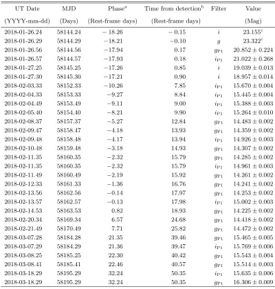
SN 2018oh is detected in PS1 g and i images, on UT 2018-01-26.56 and 26.57 (for g and i respectively), 8.9 days before the ASAS-SN discovery image, with AB magnitudes ofgP1= 20.72±0.18 andiP1= 20.94±0.25,

while the last non-detections were at UT 2018-01-23.38 and UT 2018-01-22.55. Moreover, from DECam i -band images taken one day later, SN 2018oh was i = 19.04±0.01 and 18.96±0.01 mag on 2018 Jan 27.25 and 2018 Jan 27.29, respectively, revealing a rise in the

i band of ∼1 mag in one day. A collection of ground-based images, showing pre-explosion, first detection and close-to-peak luminosity, ing and ibands, is presented in Figure1, and reported in Table1.

After correcting for the Milky Way extinction us-ing the Fitzpatrick (1999) law with RV = 3.1, we

fit the uBVgriz photometry (Li et al. 2018) with the most recent version of the _SALT2 light curve fitter

(SALT2.4;Betoule et al. 2014;Guy et al. 2010) through the SNANA framework (Kessler et al. 2009). We mea-sure a SALT2 shape parameter ofx1= 0.879±0.012 and

a color parameter of c = −0.09±0.01. We determine that SN 2018oh peaked at Bpeak = 14.185±0.010 mag

on MJD 58163.339±0.016.

To infer the distance, we use the distance estimator

fromBetoule et al.(2014), and references therein:

µ=mB−MB+α×x1−β×c+ ∆M, (1)

wheremB,x1andcare given above. We use the values

of the nuisance parameters α = 0.141, β = 3.099 and

MB =−19.17 given by Betoule et al. (2014).

Regard-ing the host galaxy mass step ∆M (Kelly et al. 2010;

Lampeitl et al. 2010;Sullivan et al. 2010), we use SDSS

g and i magnitudes with the relation of Taylor et al.

(2011, their Equation 8) to derive the host galaxy mass of UGC 4780. We find the mass to be 8.81 dex, comfort-ably on the low-mass side of the step function, and we correct with ∆M =−0.06 mag. The final distance

mod-ulus, assumingH0= 73 km s−1Mpc−1, is estimated to

beµ= 33.61±0.05 mag, corresponding to a distance of 52.7±1.2 Mpc. As UGC 4780 is not in the Hubble flow and has no independent distance measurement, the dis-tance using the SN itself is the most accurate and precise distance, and we use this distance for the remainder of the analysis.

The near-peak and post-peak photometric data of SN 2018oh show that the SN is a normal SN Ia, while the only spectral peculiarity is the (relatively) long-lived carbon absorption features, seen even to about 3 weeks after the maximum light and discussed in Li et al. (2018). From all available data, we conclude that SN 2018oh is a normal SN Ia.

3.2. Kepler Light Curve

After the reduction of the SN 2018ohKepler/K2 light curve as described in Section 2, which only provides a relative-flux light curve, we determine the true K2 flux as follows. We use the uBVgriz photometry (Li et al. 2018), which has been calibrated to the PS1 sys-tem to determine the SN 2018oh flux as a function of time and wavelength. We then use the “max model” of the SNooPy2 package (Burns et al. 2015) to deter-mine the spectral-energy distribution (SED) of the SN as a function of time. This model first fits for the peak flux in each photometric band by scaling template light curves (Burns et al. 2011) to the data, with the modelK -corrections calculated by warping theHsiao et al.(2007)

2 _{https://users.obs.carnegiescience.edu/cburns/SNooPyDocs/}

(7)

19.325 19.330 19.335 19.340 19.345 19.350

Decl. (degrees)

30" 18-01-26 UT 06:58:25.7

g > 23.32 mag - 18.21 d

18-01-26 UT 13:31:39.5

gP1 = 20.85 mag

- 17.94 d

18-02-11 UT 11:43:43.9

gP1 = 14.26 mag

- 2.19 d

136.68 136.67 136.66 136.65 19.325

19.330 19.335 19.340 19.345 19.350

Decl. (degrees)

30" 18-01-26 UT 05:39:50.4

i > 23.15 mag - 18.26 d

136.68 136.67 136.66 136.65 R.A. (degrees)

18-01-26 UT 13:43:59.4

iP1 = 21.02 mag - 17.93 d

136.68 136.67 136.66 136.65

18-02-09 UT 11:36:38.1

[image:7.612.70.541.69.381.2]

iP1 = 14.93 mag - 4.17 d

Figure 1. SN 2018ohg (top row) and i (bottom row) images of pre-explosion (left), first detection (middle) and close to

peak magnitude (right). The images are 107.500×107.500stamps from DECam (left) and PS1 (middle and right). For the first detections, we additionally show a zoom of 12.500×12.500of the difference image in the onset. We label the date of observation, time from B-band peak (in rest-frame days) and measured AB magnitude in each image stamp. The location of the SN is indicated with a tick mark (and a circle for the difference image).

SN Ia spectral series to match the observed colors. This approach accounts for assumptions about host-reddening and the distance to the SN by modeling the multi-band photometry before determining the K2 mag-nitudes. The best-fit parameters were used to normalize the mangled spectral series to the observed photometry and to generate a synthetic SED. As the Burns et al.

(2011) method mangles the spectral series to match the SED in each observer-frame passband, there is a choice of which passband’s normalized SED to use as a model for the K2 band. We use the V band as its effective wavelength is closest to that of the K2 band. After inte-grating over the K2 passband, recovering the ‘synthetic’ K2 light curve, we solve for the absolute zeropoint, us-ing the background-subtracted K2 flux light curve, in-terpolated over a range of ±3 d around the time of B -band maximum light, where the supernova color evolves slowly. We estimate ZPK2= 25.324±0.004 (statistical).

We find a ±0.011 (systematic) mag, systematic uncer-tainty arising from the choice of which (observer-frame)

passband normalized-SED is used to model the synthetic K2 light curve.

We present the SN 2018oh K2 light curve in Figure2, normalized to the peak of the light curve, which we es-timate by fitting a polynomial to the data from MJD 58160.0 to 58165.0. We find that the peak in the K2 band occurs at MJDK2max = 58162.58, ∼0.12 days prior

to B-band maximum, with K2max= 14.401±0.001. A

portion of the light curve is presented in Table2, while the complete dataset is available in the electronic edi-tion.

3.3. Basic Analysis of the K2 Light Curve

Assuming that the photospheric temperature of a SN Ia does not change significantly in the first few days af-ter explosion, the luminosity of the Rayleigh-Jeans tail of the blackbody radiation will increase with time as

(8)

−20

−15

−10

−5

0

5

10

0.0

0.2

0.4

0.6

0.8

1.0 −20

−15

−10

−5

0

5

10 Rest−frame Days Relative to K2 Peak Brightness

0.0

0.2

0.4

0.6

0.8

1.0 Normalized Flux

SN 2018oh

K2 Raw Data

K2 Binned Data (12h)

K2 first detection

Fit region

t

₀

0.0 0.1 0.2 0.3 0.4

PS1 DECam−i DECam

Non− Detection

−20 −18 −16 −14 −12

−0.01

0.00 0.01 0.02 0.03

[image:8.612.69.548.60.302.2]

Residual

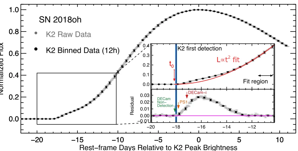
Figure 2. SN 2018oh K2 light curve, normalized to peak flux, with respect to peak brightness. Unbinned K2 photometry

and data averaged over 12 hours are shown as grey and black points, respectively. In the inset’s upper panel, we show the zoomed light curve from 20 to 10 days before peak brightness. AL∝t2 model (red line) fit to the data in the ‘Fit region’ is displayed. The residual of the fit is shown in the lower panel. The time of our last DECam non-detection, first PS1 and DECam observations are marked with green, orange and red arrows, respectively. The black vertical line corresponds to the estimation of the onset of the K2 light curve, as described in the text, with the blue-shaded region representing the 3-σstandard deviation.

an initial flux excess, from∼18 to 13 days before peak brightness, which eventually subsides and the usual “ex-panding fireball” rise dominates starting about 13 days before peak brightness.

We determine the onset of the K2 light curve as fol-lows: For a given sliding time-window, we calculate the weighted-mean of the flux and we compare it with the flux of the time-window prior to it, marking as a detec-tion when Fluxi > 3σi−1. By an iterative procedure,

using decreasing time-window widths, we record the de-tection times, and we estimate their mean and standard deviation. We calculatetK2

det=−17.99±0.04 days from

maximum light (at MJDK2_det= 58144.39), shown as the black vertical line in Figure 2. We note that the first PS1 detections were 0.18 days (4.32 hours) after the K2 first detection, which we estimate to be 2018 Jan 26.04. In order to determine the properties of the power-law rise (i.e., excluding the first-component rise), we attempt to estimate a time range by iteratively fitting, using _idl’s MPFIT function, a (t−t0)2 power law to

the data in a window from a variable (shifting by steps of 0.02 days) start time beginning 20 days before peak brightness until the flux reaches 40% of the peak flux, as has been done with other KeplerSN Ia studies (Olling

et al. 2015). Our best fit (reduced χ2 = 1.09) is for

a time window from 11.54 to 10.32 days before peak

brightness, which we mark with a vertical two-headed arrow in Figure 2. From this fit, we estimate a time of first light, t0 = −18.14±0.02 days — ∼0.15 days

(∼3.6 hours) before our first K2 detection. We display the residual to the fit in the bottom panel of the inset in Figure2. We find that ∼2 days after t0, the flux

ex-cess is∼3 times as luminous as the power-law rise, and represents∼65% of the total flux at that time.

As it has been shown in previous rise time studies

(Riess et al. 1999;Hayden et al. 2010b;Ganeshalingam

et al. 2011; Gonz´alez-Gait´an et al. 2012; Firth et al. 2015), the index of the power law can significantly vary from 2 for a particular SN. To account for this possibil-ity, we repeat the previous procedure and, usingemcee, a Python-based application of an affine invariant Markov chain Monte Carlo (MCMC) with an ensemble sampler (Foreman-Mackey et al. 2013), we fit a (t−t0)α

power-law (thus, additionally fitting for the power-power-law index). Doing so, we find a similar best-fit region as before, with the new best-fit parameterst0 =−17.86+0.24−0.25 days

be-fore peak brightness, withα= 1.92±0.07.

In order to quantify the rise of the excess flux com-ponent, and motivated by its shape, we consider a sim-ple analytical model that consists of (1) a power law

L∝(t−t0)α and (2) a skewed Gaussian to account for

(9)

SN 2018oh K2 Raw Data

K2 Binned Data (12h)

Flux Excess Full Fit

t0

0.0 0.1 0.2 0.3 0.4

Normalized Flux

t0

K2 first detection

0.00 0.01 0.02 0.03

Data

−

Power law

0 2 4 6

Rest−frame Days Since K2 First Detection −0.010

−0.0050.000 0.005 0.010

[image:9.612.327.550.61.521.2]

Residual

Figure 3. (Top) SN 2018oh K2 light curve, normalized to

peak flux, with respect to the first K2 detection. Our full fit is shown as a solid black line, while the decomposition of the fit is shown as a red line, for the SN power law flux, and a blue line, for the first rise component. The red downward arrow denotes the time of first lightt0, estimated from the

fit. (Middle) The early flux excess, plotted as the data minus the fitted power-law model. The result of the first component fit is shown as a blue line. (Bottom) The residual of the fit (data minus full model fit).

before peak brightness through the time when the flux reaches 40% of the peak flux, with both a fixed power law index of 2, and with the index allowed to float. By fixing the index toα= 2, we estimatet0=−18.00+0.03−0.02.

When simultaneously fitting for the power-law index, we findt0=−18.19±0.05 and a= 2.08±0.02. The later

fit is shown in Figure3. These results are generally con-sistent with the canonical expanding fireball model, and the initial assumption that L∝(t−t0)2 seems

reason-able given the data.

From the multi-component fit, we also estimate that the early excess flux peaked with a luminosity of (4.3± 0.2)×1037_{erg s}−1_at_tc1

peak=−16.05±0.04 days,

approx-imately 2.2 days aftert0, and had a FWHM of 3.12 days.

The total emitted energy above the power-law rise is (1.27±0.01)×1043 _erg.

3.4. Comparison to Other SNe

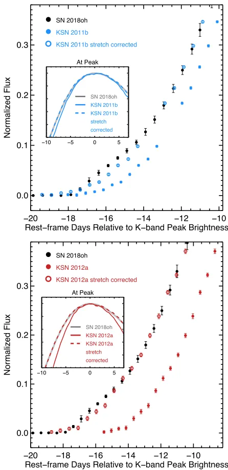
Firstly, we compare the K2 light curve of SN 2018oh with the Kepler SNe presented in Olling et al.(2015), focusing on the discovery and rise epochs (Figure 4). As mentioned inOlling et al. (2015), KSN 2011b (blue full circles) and KSN 2012a (red full circles) occurred in red and passive galaxies at redshifts∼0.05 and∼0.09 (we exclude the 3rd Kepler SN of Olling et al. 2015, KSN 2011c, due to the lower quality of data). More-over, these SNe are fast decliners (thus, have lower ab-solute luminosities) while SN 2018oh is a normal SN Ia. For this reason, we ‘stretch-correct’ (Perlmutter et al.

SN 2018oh

KSN 2011b

KSN 2011b stretch corrected

−20 −18 −16 −14 −12 −10

Rest−frame Days Relative to K−band Peak Brightness 0.0

0.1 0.2 0.3

Normalized Flux

At Peak

−10 −5 0 5

SN 2018oh KSN 2011b KSN 2011b stretch corrected

SN 2018oh KSN 2012a

KSN 2012a stretch corrected

−20 −18 −16 −14 −12 −10

Rest−frame Days Relative to K−band Peak Brightness 0.0

0.1 0.2 0.3

Normalized Flux

At Peak

−10 −5 0 5

SN 2018oh

KSN 2012a KSN 2012a stretch corrected

Figure 4. Comparison of the K2 SN 2018oh light curve

(black circles), normalized to peak, with respect to peak brightness, with KSN 2011b (upper panel) and KSN 2012a (lower panel). The Kepler light curves of KSN 2011b and KSN 2012a have been ‘stretch-corrected’ to match the SN 2018oh light curve. We show the original 12-h time binned data fromOlling et al.(2015) in full circles, and the ‘stretch-corrected’ ones with open circles. In the insets, we show a zoom of the light curves at peak.

[image:9.612.58.287.63.215.2]

(10)

As it can be seen, the applied stretch correction suc-cessfully matches the SNe at the epochs around peak brightness. However, SN 2018oh clearly deviates for the first few days after explosion, when the flux excess is observed. We estimate that, at the time of the peak of the flux excess,tc1

peak=−16.05 days, SN 2018oh is 51%

and 32% more luminous than the stretch-corrected KSN 2011b and KSN 2012a, respectively.

Next, we compare the early SN 2018oh light curves with those of two other SNe with very early data: the well-studied, extremely young SN 2011fe (Nugent et al. 2011), a normal Type Ia supernova that shows no flux excess at the extremely early times, and SN 2017cbv

(Hosseinzadeh et al. 2017), a SN Ia with a prominent

blue early flux excess. For this comparison, we need comparable filters. SN 2017cbv has extensive early-time photometry in the desiredgandibands (Hosseinzadeh

et al. 2017). SN 2011fe also has an early g-band light

curve (Nugent et al. 2011), but lacks an early i-band light curve. In place of filtered photometry, we use thePereira et al.(2013) spectrophotometric time series, from which we synthesize ani-band light curve.

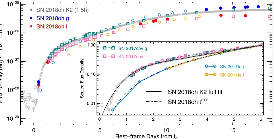
In Figure 5, we simultaneously display the early SN 2018oh K2 (gray),g(blue), andi(red) light curves. For comparison, we also show similar data for SNe 2011fe and 2017cbv. In the inset, we show the first 6 days after explosion, where the SN rose >2 orders of magnitude in flux. We also display the full two-component fit to the SN 2018oh light curve and just the power-law component.

While SN 2011fe clearly lacks the flux excess of SN 2018oh and rises close to t2, SN 2017cbv has a flux excess at early times and an early photometric behavior comparable to SN 2018oh. At later times (t > −10 days), all three SNe evolve similarly. No-tably, from that point on, SN 2018oh looks identical to the “normal” SN 2011fe.

Finally, we investigate the color evolution of SN 2018oh, and in particular theg−i,g−K2 and K2−icolors. We compare the SN 2018oh colors to the synthetic colors of SNe 2011fe and 2017cbv, calculated as described above (note that we also estimate the synthetic K2 magni-tude). Additionally, we compute the color evolution of

the Hsiao et al. (2007) template spectra. The results

are shown in Figure6.

While SNe 2018oh and 2017cbv generally have similar colors for the epochs examined here, generally having bluer colors than both SN 2011fe and the Hsiao et al.

(2007) template, there is a distinct difference at the earliest epochs, when the prominent flux excess is ob-served. We note the difference in the K2−i color, at the onset of the excess-flux component where SN 2018oh

is bluer than all comparison SNe (∼0.1 and 0.08 mag from SN 2011fe and SN 2017cbv, respectively). Unfor-tunately, we only have a singleiobservation during this phase. Nonetheless, this single observation is critical in separating SN 2018oh from SN 2017cbv.

3.5. SED of the Excess Flux

Finally, we investigate the SED of the excess flux ob-served from 18 to 13 days before peak brightness. While we have no spectra during this phase, we have filtered photometry that can constrain the SED. In addition to the K2 photometry, we will use the PS1gand DECami

observations att=−17.8 and−17.1 days, respectively which were obtained while the flux excess was still rising (see inset of Figure2).

We will focus on the crucial DECam iobservation at

t=−17.1 days from the K2 maximum, which coincides with the rise of the flux excess (see onset of Figure2). While there is no spectrum of SN 2018oh taken at that epoch, motivated by the similar peak/post-peak pho-tometric and spectroscopic behavior with SN 2011fe, we use the Lick/KAST spectrum, presented initially by

Nu-gent et al. (2011), taken ∼1.5 days after the SN 2011fe

explosion (−16.33 rest-frame days from B−band maxi-mum light). We attempt to spectroscopically match this spectrum (for which no flux excess is observed) with the photometric colors of SN 2018oh at the epoch in ques-tion. As mentioned above, we unfortunately don’t have

g observations at this epoch, therefore we assume no color evolution ing−ifor the first days (see left panel of Figure 6). We note that this assumption is some-how arbitrary: Our photometry at−17.8 days has large uncertainties, while theg−icolor is redder, compared to SN 2017cbv. Nevertheless, after redshifting the spec-trum to the redshift of SN 2018oh, we scale it to match the SN component of the K2 flux at−17.1 days, as de-termined in Section 3.3, Figure 3. We then perform a MCMC fit of this spectrum and a blackbody spectrum, where the resulting spectrum reproduces the observed photometry, with the results shown in Figure7.

Our best fit includes a blackbody withT = 17,500+11,500₋_9,000 K. The main source of the large uncertainty comes from the constant color evolution assumption and the corresponding large photometric uncertainty at this extremely early epoch. However, the resulting fitted temperature is high, providing an indication of a hot blackbody component, on top of the normal SN spec-trum.

4. MODELS

(11)

two-SN 2018oh K2 (1.5h) SN 2018oh g

SN 2018oh i

0 5 10 15

Rest−frame Days from t0 10−29

10−28 10−27 10−26 10−25

Flux Density (erg s

−

1 Hz

−

1 cm

−

2 )

SN 2018oh K2 full fit

SN 2018oh t2.08

SN 2011fe g

SN 2011fe i

SN 2017cbv g

SN 2017cbv i

0 1 2 3 4 5 6

0.01 0.10 1.00

[image:11.612.72.543.78.317.2]

Scaled Flux Density

Figure 5. SN 2018oh flux ingP1(blue),iandiP1(red) and K2 (gray), with respect to the rest-frame time since first light,t0,

as estimated in Section3.3. Non-detections in the K2 band are plotted as open gray circles. Similar light curves for SN 2011fe (g and syntheticiP1) and SN 2017cbv (gandi) are also shown, after being normalized to the appropriate peak flux of SN 2018oh.

(Inset) A zoomed-in region of the extremely early light curve, normalized to the K2 flux at 6 days after explosion. Note that the comparison SN sample is additionally plotted as solid (SN 2011fe) and dashed (SN 2017cbv) lines, with some of the photometric points removed for clarity. We overplot the fits described in Section3as indicated in the legend.

SN 2018oh PS1 SN 2018oh DECam SN 2018oh Swope SN 2018oh PS1 SN 2018oh DECam SN 2018oh Swope

SN 2011fe

SN 2017cbv

Hsiao 2007 SN 2011fe

SN 2017cbv

Hsiao 2007

-20 -10 0 10 20

Phase (rest-frame days) -1.2

-1.0 -0.8 -0.6 -0.4 -0.2 -0.0

g - i

Epoch of Flux Excess Epoch of Flux Excess

-20 -10 0 10 20

-0.2 0.0 0.2 0.4

g - K2

-20 -10 0 10 20

-0.4 -0.2 0.0 0.2

K2 - i

Figure 6. g−i(left),g−K2 (middle) and K2−i(right) color curves for SN 2018oh. We additionally include data from the

[image:11.612.73.540.447.635.2]

(12)

Observed Flux SN flux SN+BB flux

Black Body TBB = 17,500 +11,500 K

Black Body TBB = 17,500 −9,000

4000 5000 6000 7000 8000 9000

Observed Wavelength (Å) 0.0

0.5 1.0 1.5 2.0

Flux Density (10

−

16 erg s

−

1 Å

−

1 cm

−

2)

gP1 K2

i

[image:12.612.57.288.57.215.2]

Response Function

Figure 7. The +1.5 day from explosion SN 2011fe spectrum

(solid black line), redshifted and scaled to match thet2.08SN component of the SN 2018oh K2 photometry at +1.09 days after t0, obtained from the fit shown in Figure3. The gP1

(blue), K2 (orange) andi(red) photometry are shown as full diamonds, at each filter’s effective wavelength. The solid green line is the best-fit blackbody spectrum that repro-duces the observed photometric colors at +1.09 days aftert0

(full circles), with the open circles representing the synthetic fluxes of the resulting spectrum (dashed line). In the upper panel, we show the response functions of thegP1(blue), K2

(orange) and DECami(red) filters.

component rise seen in the SN 2018oh light curve: the in-teraction between the SN and a nearby companion star, a double-detonation model with 56_{Ni near the surface}

of the star, and an additional model in which we tune that amount of surface56_{Ni in an attempt to best match}

SN 2018oh.

4.1. Interaction with a companion star

One potential explanation for the early-time excess is shock-interaction between the supernova ejecta and a non-degenerate binary companion (Kasen 2010). The collision is characterized by prompt X-ray emission, fol-lowed by an optical/UV excess lasting about one week after explosion. Although the excess peaks in the UV, a measurable signature is observable in theKepler band-pass if the system is configured in a favorable viewing angle (Olling et al. 2015).

To test this scenario, we use a numerical model for the early light curve following the methods outlined inPiro

& Morozova (2016) (using the Chandrasekhar

progen-itor models from Mart´ınez-Rodr´ıguez et al. 2016) that roughly matches the rise of SN 2018oh, and then com-bine this with the analytic interaction model of Kasen

(2010). The interaction emission is mainly controlled through two parameters, the orbital separation a and the characteristic ejecta velocityv. Sinceacan vary by many orders of magnitude and v is relatively well

con-strained to bev≈109_{cm s}−1_{, this makes the interaction}

a powerful diagnostic for measuringa. In addition, there are viewing angle effects, but this is somewhat degener-ate with the other parameters. Thus we focus on the the case when one is observing directly into the shocked region (when the companion is roughly between the ex-plosion and the observer) and take the measuredaas a lower limit to the orbital separation.

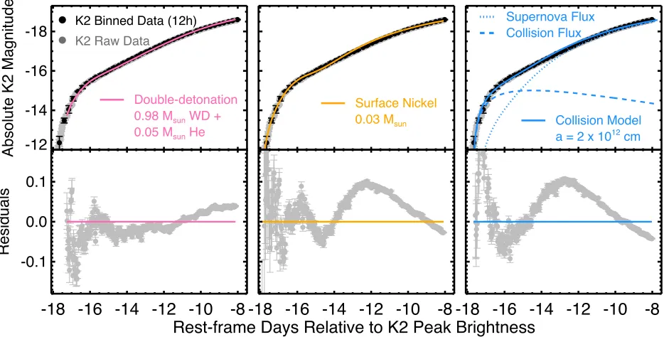
From this procedure, we find that a collision with a companion at a = 2×1012cm provides a reasonable match to the early rise. We plot this as a solid blue line in the right panel of Figure 8, and also show the con-stituent parts of the interaction (dashed blue line) and the SN itself (dotted blue line). An important assump-tion of this model is that the companion is overfilling its Roche lobe and therefore we can approximate its radius as (Eggleton 1983)

R= 0.49q

2/3

0.6q2/3_{+ ln(1 +}_q1/3₎a, (2)

where qis the ratio of the companion and WD’s mass. For a range of companion masses fromM ≈1−6 M, this results inR≈10−15 R, respectively. This is gen-erally too large for a main sequence star, and thus we conclude that the companion must be a subgiant if in-teraction is the correct explanation for the early excess. 4.2. Double-detonation sub-Chandrasekhar explosion

Another possible mechanism for creating an early-time flux excess is the double-detonation scenario for ex-ploding a sub-Chandrasekhar mass C/O WD with an ac-creted shell of helium on its surface. In this scenario, the helium shell detonates, producing on the surface some abundance of radioactive elements such as 56_{Ni and} 48_{Cr, and sending a shockwave into the WD that then}

ignites the C/O core (Woosley & Weaver 1994). The result produces observables generally consistent with a SN Ia, however, the amount of Fe-group elements syn-thesized during the He-shell detonation must be small to resemble SNe Ia near peak brightness. The photons produced by the radioactive decay of material on the surface quickly diffuse out of the ejecta, creating a flux excess relative to a typical SN Ia in the first few days after explosion (Noebauer et al. 2017).

We test this scenario as a candidate for SN 2018oh by exploring a hydrodynamic and radiative transfer numer-ical survey of double-detonations of sub-Chandrasekhar mass white dwarfs, the results of which are presented in

Polin et al.(2018). The parameter space of the survey

(13)

-12

-14

-16

-18

Absolute K2 Magnitude

K2 Binned Data (12h) K2 Raw Data

Double-detonation 0.98 Msun WD + 0.05 Msun He

-18 -16 -14 -12 -10

-8

-0.1

0.0

0.1 Residuals

Surface Nickel

0.03 Msun

-18 -16 -14 -12 -10

-8

Rest-frame Days Relative to K2 Peak Brightness

Collision Model

a = 2 x 1012_cm

Supernova Flux Collision Flux

[image:13.612.72.539.66.303.2]

-18 -16 -14 -12 -10

-8

Figure 8. The absolute magnitude K2 early-time light curve of SN 2018oh (grey and black circles). We overplot our best-fit

models, as described in Section4, of the double-detonation of a 0.98 MWD with a 0.05 MHe layer on its surface (left panel, solid pink), of a near-Chandrasekhar mass WD explosion with a surface layer of 0.03 M Nickel (middle panel, solid orange) and of a collision model (Kasen 2010) with a non-degenerate companion at a distance of a= 2×1012 _{cm (right panel, solid}

blue). We show the decomposition of the collision model to the contribution of the SN flux (dotted blue) and the interaction of the SN ejecta with the companion (dashed blue). The residuals of the model fits are shown in the lower panels.

χ2 _{measurement, is a 0.98 M}

WD with 0.05 M of Helium on its surface, with the ejecta smoothed over a mixing length of 0.25 M. This model produces a total of 0.448 M of 56Ni, 3.65×10−3 M of 48Cr and 1.8×10−2Mof52Fe. From these elements, the amount of each that is synthesized in the helium shell (i. e., in the outer layers of ejecta) is 1.22×10−2_{, 3.19}_×₁₀−2_and

6.11×10−2 _M

, corresponding to 2.7, 87.4 and 33.9%, respectively. The K2 synthetic light curve is shown in the left panel of Figure8. The approximate magnitudes of both the early-time excess and peak are reproduced, as is the duration of the excess and rise time to peak brightness.

4.3. A general off-center nickel distribution

The previous model is specifically applicable to the DD scenario, but it is possible in principle that other scenarios may mix56Ni to the outermost layers. To ex-plore this possibility more generally, we consider models in which we take a normal SN Ia explosion and place by hand some amount of 56Ni near the surface. As with the supernova model for the interaction scenario, we use the methods outlined in Piro & Morozova (2016) with the progenitors generated in the work of Mart´ınez-Rodr´ıguez et al.(2016). Using this we place the56_{Ni in}

two distinct regions, a centrally concentrated region that

provides the main rise and a shallow region above a mass coordinate of 1.3 M. The shallow abundance is varied to find the best fit with the K2 photometry, including smoothing with a 0.05 M boxcar which prevents nu-merical issues from sharp compositional gradients.

Our best-fit model under this scenario has 0.03 M of 56_{Ni near the surface of the WD as shown by the orange}

solid line in the middle panel of Figure 8. The model reproduces the general evolution of the light curve, en-capsulating the initial flux excess. We therefore pro-visionally consider this a viable model. Whether or not such a model can reproduce the full photometric and spectroscopic evolution of SN 2018oh is less clear. Iron-peak elements at shallow depths can provide exten-sive line-blanketing that alters the colors and spectra of the SN at peak luminosity, potentially making it diffi-cult for SN 2018oh to be a spectroscopically normal SN Ia. Below we consider in further detail whether such a model can even reproduce the early color evolution of SN 2018oh.

4.4. Detailed Model Comparisons

(14)

de-tections by PS1 and DECam are particularly powerful for this purpose.

In addition to detecting the flux excess in the K2 band, we also detect an excess in the i band (see Figure 5). Examining the K2−i color during the flux excess, we find that SN 2018oh is bluer than SN 2011fe by almost 0.2 mag. Moreover, SN 2018oh is also similarly bluer than SN 2017cbv at that epoch. This means that one day after explosion, SN 2018oh is not only distinct from the normal SN 2011fe but also from SN 2017cbv, which also had an early-time flux excess (Hosseinzadeh et al. 2017). After the onset of the canonical SN rise (right-wards of the grey-shaded region in the panels of Fig-ure6), the three SNe evolve in a similar manner (apart from the usual color dispersion seen in Type Ia super-novae).

All models examined above are able to reproduce the flux excess at early times of SN 2018oh, but with two main different physical origins. These models pre-dict very different SEDs and in particular different col-ors. Specifically the companion-interaction model is ex-pected to be bluer than the surface-Ni model.

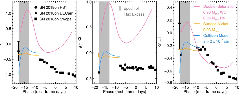
We display the expectedg−i,g−K2 and K2−i col-ors for each model in Figure 9. The double-detonation model is particularly red, and it is unable to explain the blue colors of SN 2018oh. Moreover, sub-Chandrasekhar double-detonations also leave spectral signatures such as a significant TiIIabsorption features in the peak spec-tra, that are not seen in SN 2018oh (Li et al. 2018). The generic off-center56_{Ni model also has a color that is}

red-der than SN 2018oh by ∼0.1 mag. On the other hand, the companion-interaction model with a companion at ≈2×1012_{cm generally matches both the early rise and}

the color evolution of SN 2018oh.

Based on the color evolution of SN 2018oh, we slightly favor the companion-interaction model over other mod-els that can also reproduce the early flux excess. A di-rect prediction of this model is the presence of hydrogen and/or helium-rich material stripped from the compan-ion star at the nebular phases (Pan et al. 2012;Liu et al. 2013). To this end, detections of H or He features at late-time spectra of SN 2018oh is crucial to confirm this model.

We note that, while SN 2018oh has an exquisite K2 light curve, we lack the detailed color information to conclusively decide between models, particularly at bluer wavelengths. Additionally there are no spectra of SN 2018oh during the flux excess, which would have provided key information for understanding how spec-tral features affect the color evolution. We do not see an abrupt flux excess on the first rise component, but rather a linear rise similar to other SNe Ia with

sufficiently early, high-cadence photometry that also have two-component rising light curves (e.g., SN 2012fr, which arguably shows no signs of interaction;Contreras

et al. 2018) argues against the interaction model. A

lin-ear rise may result from a particular interaction model (i.e., specific viewing angle, radius, and/or separation), however an exploration of how different parameter com-binations affect the detailed rise behavior is beyond the scope of this paper.

However, another interpretation of the flux excess is possible. Given the growing sample of SNe Ia that show two-component early light curves, with different slopes and durations, the distinct early light curve evolution of SN 2018oh, compared to the total SN Ia population, could not be due to some external heating source, but rather a reflection of varying SNe Ia properties, such as the density profile of the ejecta, different composi-tion/metallicity of the progenitor star, asymmetries dur-ing the explosion etch (seeStritzinger et al. 2018, for a relevant discussion). Modern transient surveys, such as ASAS-SN and ZTF, and future powerful surveys, such as LSST, will discover very young SNe Ia, and with rapid follow-up, the early-light curve SN sample will increase, allowing us to investigate this possibility.

5. DISCUSSION AND CONCLUSIONS In this paper, we analyze the early photometric ob-servations of SN 2018oh, a normal SN Ia, that occurred within the Kepler Campaign 16 field. The SN was observed with unprecedented cadence by the K2 SCE with complementary early Pan-STARRS1 and DECam imaging. The combination of an extremely early detec-tion and unprecedented continuous coverage with Ke-pler make SN 2018oh a spectacular reference object for early SN Ia studies, providing invaluable insights on the explosion physics and the progenitor system.

In the SN 2018oh K2 and i-band light curves, we de-tect a distinct flux component in the first few days after explosion relative to other well-observed SNe Ia (e.g., SN 2011fe) and the t2 luminosity rise seen later in the evolution of SN 2018oh. This flux excess lasts approxi-mately 5 days, after which SN 2018oh appears to evolve in a fashion consistent with typical SNe Ia.

Our work provides new insights on the early time evo-lution of SNe Ia, for which we find the following:

1. The early K2 light curve shows a distinct two-component rise evolution. Initially, the SN rises quickly, with a steep linear gradient, in flux. This flux subsides after about 5 days, when a L ∝ t2

(15)

SN 2018oh PS1 SN 2018oh DECam SN 2018oh Swope

Epoch of Flux Excess Epoch of Flux Excess

Double−detonation 0.98 Msun WD

0.05 Msun He Surface Nickel 0.03 Msun Collision Model

a = 2 x 1012_cm

−20 −15 −10 −5 0 5 10

Phase (rest−frame days)

−1.0

−0.5 0.0 0.5 1.0

g

−

i

−20 −15 −10 −5 0 5 10

−0.5 0.0 0.5 1.0

g

−

K2

−20 −15 −10 −5 0 5 10

−0.8

−0.6

−0.4

−0.2 0.0 0.2 0.4

K2

−

[image:15.612.72.541.68.252.2]

i

Figure 9. Same as Figure6 (note the different ranges in the axes), but comparing with the predicted colors of the

double-detonation model (pink), the Nickel-surface model (orange) and the collision model (blue).

2. Using thet2 _{component of the K2 light curve, we}

constrain t0 to be −18.19±0.09 days before K2

peak brightness. This time is consistent with the onset of the flux excess, indicating that both com-ponents began at the same time.

3. Assuming that the t2 _{component exists while the}

other component is bright, we find that the early flux excess peaks 2.14 days after t0, has a FWHM

of 3.12 days, a blackbody temperature of 17,500 K, a peak luminosity of 4.3×1037 _{erg/s, and a total}

emitted energy of 1.3×1043_erg.

4. We observed SN 2018oh with Pan-STARRS1 and DECam only 4.1 and 20.6 hours after the first K2 detection, respectively, providing some of the ear-liest colors of a SN Ia ever. The flux excess is confirmed in our ground-based ilight curve. 5. The SN 2018oh early photometric evolution is

rel-atively similar to SN 2017cbv, another SN Ia with a prominent two-component rising light curve. However, SN 2018oh shows bluer K2 −i colors than SN 2017cbv. This is especially true dur-ing the epoch of the initial flux excess. Around peak brightness, SN 2018oh is similar to both SNe 2011fe and 2017cbv.

6. The early flux excess can potentially be explained by additional heating at the epoch in question. We investigate three possible sources:

(a) The interaction with a non-degenerate com-panion at a = 2 ×1012_{cm, with a} _M _≈

1−6 M Roche-lobe-filling star.

(b) The presence of a 0.05 M Helium shell on the surface of 0.98 M C/O WD, and a sub-sequent sub-Chandrasekhar mass explosion. (c) An off-center56_{Ni distribution of 0.03 M}

. All of these models can, generally, reproduce the early shape of the K2 light curve. We slightly favor the interaction scenario, due to the blue colors at the epoch of the flux excess. However, another in-terpretation of the flux excess considers an intrin-sic variation of early time behavior, due to varying SNe Ia properties, with no external heating source required.

While a SD origin for (at least a sizable fraction of) SNe Ia has been previously proposed (Sternberg et al. 2011;Foley et al. 2012b;Maguire et al. 2013), its validity has been questioned. Most SNe that have some obser-vational evidence for the presence of a non-degenerate companion are either peculiar (e.g., SNe Ia-CSM; Dil-day et al. 2012; Silverman et al. 2013; Fox et al. 2015) or have contradictory observations (Shappee et al. 2018;

Sand et al. 2018). The general progenitor picture that

has emerged over the last decade is that most SNe Ia have a DD origin (Maoz et al. 2014).

(16)

investigate correlations of the light curve evolution with various SNe Ia properties.

The K2 SCE has finished and the data are currently collected and analysed. With some luck, we will soon have additional K2-observed SNe Ia with data similar in quality to that of SN 2018oh.

We will continue to monitor SN 2018oh. Late-time observations, after the SN has become optically thin, will be a direct test of our proposed models.

We thank the anonymous referee for helpful comments that improved the clarity and presentation of this paper. This paper includes data collected by the K2 mission. Funding for the K2 mission is provided by the NASA Science Mission directorate.

KEGS is supported in part by NASA K2 cycle 4 and 5 grants NNX17AI64G and 80NSSC18K0302, respec-tively. AR and his groups is supported in part by HST grants GO-12577 and HST AR-12851.

Pan-STARRS (PS1) is supported in part by the Na-tional Aeronautics and Space Administration under Grants NNX12AT65G and NNX14AM74G. The Pan-STARRS1 Surveys (PS1) and the PS1 public science archive have been made possible through contributions by the Institute for Astronomy, the University of Hawaii, the Pan-STARRS Project Office, the Max-Planck Soci-ety and its participating institutes, the Max Planck In-stitute for Astronomy, Heidelberg and the Max Planck Institute for Extraterrestrial Physics, Garching, The Johns Hopkins University, Durham University, the Uni-versity of Edinburgh, the Queen’s UniUni-versity Belfast, the Harvard-Smithsonian Center for Astrophysics, the Las Cumbres Observatory Global Telescope Network Incorporated, the National Central University of Tai-wan, the Space Telescope Science Institute, the National Aeronautics and Space Administration under Grant No. NNX08AR22G issued through the Planetary Science Division of the NASA Science Mission Directorate, the National Science Foundation Grant No. AST–1238877, the University of Maryland, Eotvos Lorand University (ELTE), the Los Alamos National Laboratory, and the Gordon and Betty Moore Foundation.

This project used data obtained with the Dark En-ergy Camera (DECam), which was constructed by the Dark Energy Survey (DES) collaboration. Funding for the DES Projects has been provided by the DOE and NSF (USA), MISE (Spain), STFC (UK), HEFCE (UK), NCSA (UIUC), KICP (U. Chicago), CCAPP (Ohio State), MIFPA (Texas A&M), CNPQ, FAPERJ, FINEP (Brazil), MINECO (Spain), DFG (Germany) and the collaborating institutions in the Dark Energy

Survey, which are Argonne Lab, UC Santa Cruz, Uni-versity of Cambridge, CIEMAT-Madrid, UniUni-versity of Chicago, University College London, DES-Brazil Con-sortium, University of Edinburgh, ETH Z¨urich, Fer-milab, University of Illinois, ICE (IEEC-CSIC), IFAE Barcelona, Lawrence Berkeley Lab, LMU M¨unchen and the associated Excellence Cluster Universe, University of Michigan, NOAO, University of Nottingham, Ohio State University, OzDES Membership Consortium, University of Pennsylvania, University of Portsmouth, SLAC Na-tional Lab, Stanford University, University of Sussex, and Texas A&M University.

Based on observations at Cerro Tololo Inter-American Observatory, National Optical Astronomy Observatory (NOAO 2017B-0279; PI: A Rest, NOAO 2017B-0285; PI: A Rest), which is operated by the Association of Universities for Research in Astronomy (AURA) under a cooperative agreement with the National Science Foun-dation.

The UCSC group is supported in part by NASA grants NNG17PX03C and 80NSSC18K0303, NSF grants AST-1518052 and AST-1815935, the Gordon & Betty Moore Foundation, the Heising-Simons Foundation, and by fel-lowships from the Alfred P. Sloan Foundation and the David and Lucile Packard Foundation to R.J.F.

We thank Chris Burns for providing crucial updates toSNooPy, relevant to the analysis of this work.

SJS acknowledges funding from STFC Grants ST/P000312/1 and ST/N002520/1.

This work makes use of observations from Las Cum-bres Observatory. DAH, CM, and GH are supported by the US National Science Foundation grant 1313484. Support for IA was provided by NASA through the Ein-stein Fellowship Program, grant PF6-170148.

JV and his group at Konkoly Observatory is sup-ported by the project “Transient Astrophysical Objects” GINOP 2.3.2-15-2016-00033 of the National Research, Development and Innovation Office (NKFIH), Hungary, funded by the European Union.

This project has been supported by the Lend¨ulet Pro-gram of the Hungarian Academy of Sciences, projects No. LP2018-7/2018 and LP2012-31, and the NKFIH grant K-115709.

ZsB acknowledges the support provided from the Na-tional Research, Development and Innovation Fund of Hungary, financed under the PD 17 funding scheme, project no. PD123910.

Research by DJS is supported by NSF grants AST-1821967, 1821987, 1813466 and 1813708. NS and JEA received support from NSF grant AST-1515559.

(17)

for the LJT has been provided by Chinese Academy of Sciences and the People’s Government of Yunnan Province. The LJT is jointly operated and adminis-trated by Yunnan Observatories and Center for Astro-nomical Mega-Science, CAS. This work is supported by the National Natural Science Foundation of China (NSFC grants 11178003, 11325313, and 11633002), and the National Program on Key Research and Develop-ment Project (grant no. 2016YFA0400803). JJZ is sup-ported by the National Science Foundation of China (NSFC, grants 11403096, 11773067), the Youth Inno-vation Promotion Association of the CAS, the Western Light Youth Project, and the Key Research Program of the CAS (Grant NO. KJZD-EW-M06). TMZ is sup-ported by the NSFC (grants 11203034). This work was also partially Supported by the Open Project Program of the Key Laboratory of Optical Astronomy, National

Astronomical Observatories, Chinese Academy of Sci-ences.

EB and JD acknowledge partial support from NASA grant NNX16AB5G.

CPG acknowledges support from EU/FP7-ERC grant No. [615929].

Parts of this research were supported by the Aus-tralian Research Council Centre of Excellence for All Sky Astrophysics in 3 Dimensions (ASTRO 3D), through project number CE170100013.

Support for this work was provided by NASA through Hubble Fellowship grant #HST-HF2-51357.001-A, awarded by the Space Telescope Science Institute, which is operated by the Association of Universities for Re-search in Astronomy, Incorporated, under NASA con-tract NAS5-26555, as well as NASA K2Cycle 4 Grant NNX17AE92G.

APPENDIX

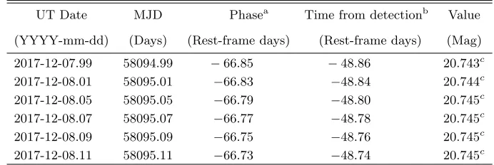
A. PHOTOMETRY TABLES

REFERENCES

Arnett, W. D. 1982, ApJ, 253, 785

Barentsen, G., & Cardoso, J. V. d. M. 2018, Kadenza: Kepler/K2 Raw Cadence Data Reader, Astrophysics Source Code Library, , , ascl:1803.005.

https://doi.org/10.5281/zenodo.344973

Betoule, M., Kessler, R., Guy, J., et al. 2014, A&A, 568, A22

Bianco, F. B., Howell, D. A., Sullivan, M., et al. 2011, ApJ, 741, 20

Bloom, J. S., Kasen, D., Shen, K. J., et al. 2012, ApJL,

744, L17

Brown, J. S., Stanek, K. Z., Vallely, P., et al. 2018, The Astronomer’s Telegram, 11253

Brown, P. J., Dawson, K. S., Harris, D. W., et al. 2012, ApJ, 749, 18