Ji_unc_0153D_17356.pdf

DATA-DRIVEN 3D RECONSTRUCTION AND VIEW SYNTHESIS OF DYNAMIC SCENE ELEMENTS

Dinghuang Ji

A dissertation submitted to the faculty of the University of North Carolina at Chapel Hill in partial fulfillment of the requirements for the degree of Doctor of Philosophy in the Department of

Computer Science.

Chapel Hill 2017

©2017 Dinghuang Ji

ABSTRACT

Dinghuang Ji: Data-driven 3D Reconstruction and View Synthesis of Dynamic Scene Elements (Under the direction of Jan-Michael Frahm and Enrique Dunn)

Our world is filled with living beings and other dynamic elements. It is important to record dynamic things and events for the sake of education, archeology, and culture inheritance. From vintage to modern times, people have recorded dynamic scene elements in different ways, from sequences of cave paintings to frames of motion pictures. This thesis focuses on two key computer vision techniques by which dynamic element representation moves beyond video capture: towards 3D reconstruction and view synthesis. Although previous methods on these two aspects have been adopted to model and represent static scene elements, dynamic scene elements present unique and difficult challenges for the tasks.

This thesis focuses on three types of dynamic scene elements, namely 1) dynamic texture with static shape, 2) dynamic shapes with static texture, and 3) dynamic illumination of static scenes. Two research aspects will be explored to represent and visualize them: dynamic 3D reconstruction and dynamic view synthesis. Dynamic 3D reconstruction aims to recover the 3D geometry of dynamic objects and, by modeling the objects’ movements, bring 3D reconstructions to life. Dynamic view synthesis, on the other hand, summarizes or predicts the dynamic appearance change of dynamic objects – for example, the daytime-to-nighttime illumination of a building or the future movements of a rigid body.

computer vision. To perform this 3D reconstruction, we introduce a method that simultaneously 1) segments dynamically textured scene objects in the input images and 2) reconstructs the 3D geometry of the entire scene, assuming a static 3D shape for the dynamically textured objects.

Compared to dynamic textures, the appearance change of dynamic shapes is due to physically defined motions like rigid body movements. In these cases, assumptions can be made about the object’s motion constraints in order to identify corresponding points on the object at different timepoints. For example, two points on a rigid object have constant distance between them in the 3D space, no matter how the object moves. Based on this assumption of local rigidity, we propose a robust method to correctly identify point correspondences of two images viewing the same moving object from different viewpoints and at different times. Dense 3D geometry could be obtained from the computed point correspondences. We apply this method on unsynchronized video streams, and observe that the number of inlier correspondences found by this method can be used as indicator for frame alignment among the different streams.

To model dynamic scene appearance caused by illumination changes, we propose a framework to find a sequence of images that have similar geometric composition as a single reference image and also show a smooth transition in illumination throughout the day. These images could be registered to visualize patterns of illumination change from a single viewpoint.

ACKNOWLEDGEMENTS

My deepest gratitude is to my advisors Jan-Michael Frahm and Enrique Dunn, for the discus-sions and guidence they gave in countless meetings, for the patience and encouragement when I encounter failures, and for the endless support in my program study and job hunting.

I would also like to thank my committee members, Tamara L. Berg, Marc Niethammer, and Silvio Savarese, for their feedback and advice.

Additionally, I would like to thank my labmates, as their company and discussion made my time more fruitful and enjoyable:

Philip Ammirato, Akash Bapat, Sangwoo Cho, Marc Eder, Pierre Fite-Georgel, Yunchao Gong, Rohit Gupta, Shubham Gupta, Xufeng Han, Jared Heinly, Junpyo Hong, Hadi Kiapour, Hyo Jin Kim, Wei Liu, Licheng Yu, Vicente Ord´o˜nez-Rom´an, David Perra, True Price, Rahul Raguram, Patrick Reynolds, Johannes Sch¨onberger, Meng Tan, Joseph Tighe, Sirion Vittayakorn, Ke Wang, Yilin Wang, Zhen Wei, Yi Xu, Hongsheng Yang, and Enliang Zheng.

I deeply appreciate my mentors during internships, for their kind support and supervision: Shiyu Song, Yong-Dian Jian, and Junghyun Kwon.

I want to thank my friends met in Chapel Hill, who really made me enjoy the life and taught me how to become a better person: Yi Hong, Wentao Li, Michael Wilson, Hongxiang Long, Jun Jiang, Qiuyu Xiao, Yu Meng, Yipin Zhou, Jingbo Wang, Wenhua Guan, Ye Zhao, Ruoyu Wu, Xiaoming Liu, Dawei Tang, Cheng Cao, Yueting Luo, Xiaodan Wang, Qingning Zhou, Qixin Wu, Wenshuai Li, Si Chen, and Mark Vance. I especially appreciate Yirong Jia, Baocai Cheng, Yu Cheng and James Wang for their long lasting friendship and supports.

TABLE OF CONTENTS

LIST OF TABLES . . . ix

LIST OF FIGURES . . . x

LIST OF ABBREVIATIONS . . . xiv

1 Introduction . . . 1

1.1 Thesis Statement . . . 4

1.2 Outline of Contributions . . . 5

2 Related work . . . 8

2.0.1 3D Reconstruction of Dynamic Objects . . . 8

2.0.2 Appearance Analysis and Mosaics . . . 12

2.0.3 View Synthesis and Visual Predictions . . . 14

3 3D Reconstruction of Dynamic Textures in Crowd Sourced Data . . . 16

3.1 Introduction . . . 16

3.2 Initial Model Generation . . . 18

3.2.1 Static Reconstruction from Photo Collections . . . 18

3.2.2 Coarse Dynamic Textures Priors from Video . . . 18

3.2.3 Coarse Static Background Priors from Video Frames . . . 20

3.2.4 Graph-cut based dynamic texture refinement . . . 21

3.2.5 Shape from silhouettes . . . 22

3.3 Closed Loop 3D Shape Refinement . . . 24

3.3.1 Geometry based Video to Image Label Transfer . . . 24

3.3.3 Building a Static Background Prior for Single Images . . . 26

3.3.4 Mitigating of Non-uniform Spatial Sampling . . . 28

3.4 Experiments . . . 29

3.5 Conclusion . . . 32

4 Spatio-Temporally Consistent Correspondence for Dense Dynamic Scene Modeling . . . 33

4.1 Introduction . . . 33

4.2 Spatio-Temporal Correspondence Assessment . . . 34

4.2.1 Notation . . . 35

4.2.2 Pre-processing and Correspondence Formulation . . . 35

4.2.3 Assessment and Correction Mechanism . . . 38

4.2.3.1 Step

¶

4.2.3.2 Step

·

4.2.3.3 Step

¸

4.2.3.4 Step

¹

4.2.4 Applications to Stream Sequencing and 3D Reconstruction . . . 42

4.3 Experiments . . . 43

4.4 Discussion and Conclusion . . . 45

5 Synthesizing Illumination Mosaics from Internet Photo-Collections . . . 48

5.1 Introduction . . . 48

5.2 Illumination Mosaic Generation . . . 50

5.2.1 Data Collection and Pre-Processing . . . 51

5.2.2 Defining the Illumination Spectrum . . . 51

5.2.3 Image Sequence Generation . . . 52

5.2.4 Homography-Based Image Stitching . . . 54

5.2.5 Image Blending . . . 56

6 Dynamic Visual Sequence Prediction with Motion Flow Networks . . . 65

6.1 Introduction . . . 65

6.2 Our Approach . . . 67

6.2.1 MotionFlowNet: Appearance Flow Estimation for Sequence Synthesis . . . 68

6.2.2 PoseFlowNet: Appearance Flows with Constrained Directions . . . 70

6.2.3 Implementation details . . . 74

6.3 Experiments . . . 74

7 Discussion . . . 82

7.1 Future work . . . 82

7.1.1 Extensions to 3D Reconstruction of Dynamic Texture . . . 82

7.1.2 Extensions to 3D Reconstruction of Dynamic Shapes . . . 83

7.1.3 Extensions to View Synthesis . . . 84

LIST OF TABLES

3.1 Composition of our downloaded crowd sourced datasets . . . 29 4.1 Composition of our datasets. . . 44 5.1 Composition of our downloaded image datasets. The number of clustered

images corresponds to images that were able to register through geometric verification to their cluster center. In most cases (˜90%), stripe reordering is applied to generate smoother appearance transition (For Notre Dame dataset,

stripe reordering didn’t change its original sequence). . . 60 5.2 For each dataset, we create three sequences with different reference images

and compute our predefined values. For Trevi Fountain I&II and Coliseum, Rome I&II, they differ in the viewing angle. Bold-font numbers highlight the best matching score, eight out of the ten datasets achieve the best results using

our method. For the other two datasets, we are very close to the best scores. . . 61 6.1 All convolution layers are followed by ReLU. FC1 layer is followed by ReLU

and dropout. k: kernel size (kxk). s: stride in horizontal and vertical directions. c: number of output channels. h: number of output heights. w: number of output widths. d: output spatial dimension. Conv: convolution. Deconv:

deconvolution. IP: InnerProduct. . . 75 6.2 MSE testing error for different frames in human3.6m (top four rows) and

Sprites (bottom two rows) dataset. . . 79 6.3 End positions – Motion flow direction prediction error for different frames in

human3.6m dataset. The values are in the unit of pixels and degrees. . . 79 6.4 RelAng – RelLen testing error for different frames in human3.6m dataset. The

values are in the unit of degrees and pixels. . . 80 6.5 MoFlowNet testing errors with different input images for frame 5 and 6 on

LIST OF FIGURES

3.1 Workflow overview of the proposed framework. . . 17 3.2 Keyframe selection for an input video. The plot shows the frame number count

vs the NCC similarity of each frame’s HOG descriptor. Red boxes indicate selected video fragments centered on sampled frames. Keyframe selection is a

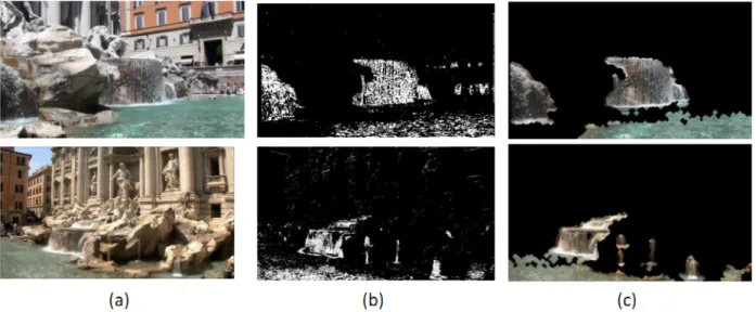
function of the plot density at the upper end of the NNC values. . . 20 3.3 Dynamic content priors from video fragments. Left to right: (a) Reference

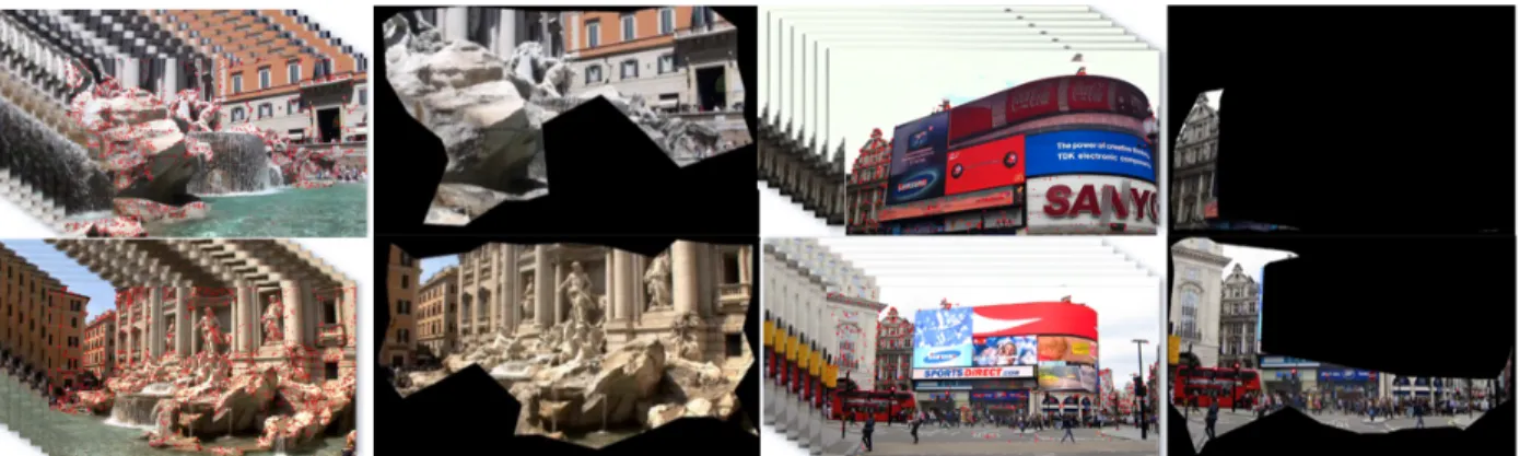
frame (b) Accumulated frame differencing (c) Result after post processing. . . 20 3.4 Static content prior from video fragments. First and third columns depict SIFT

features matches among neighboring frames as red dots. Second and fourth columns depict the concave hull defined by detected features not overlapping

with the existing dynamic content prior. . . 21 3.5 Graphh-cut label refinement. First and third rows depict (alternatively from

left to right) single image dynamic and static content priors. Second and fourth rows depict the outputs of the label optimization, where green regions are

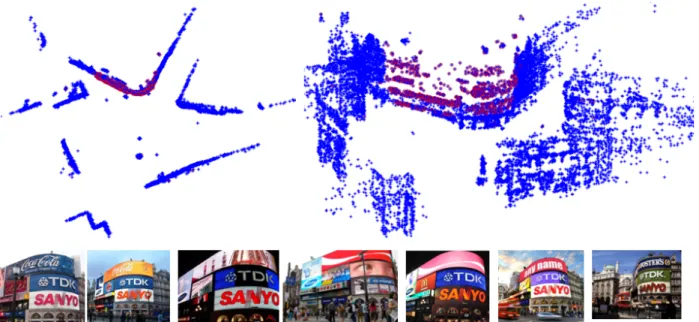
dynamic textures. . . 23 3.6 Identification of dynamic textures within existing SfM estimates.Top Row:

birds-eye and fontal view of estimated sparse structure for Piccadilly Circus. Blue dots are 3D features with persitent color across the dataset. Red dots are 3D features determined to have sporadic color. The bottom row shows sample images in the dataset. We associate color persistance with predominantly linear

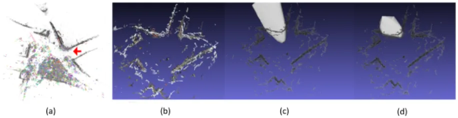
variation in the RGB space. . . 27 3.7 Mitigation of non uniform spatial sampling. Left to right: (a) Cameras in

the red arrow direction are scarse in the SfM model (b) Quasi-dense output from PMVS (c) Dynamic Shape estimation with uniformly weighted carving. the reconstructed 3D volume will be towards the cmera centroid (d) Shape

estimate with weighted carving. . . 28 3.8 Evolution of estimated 3D dynamic content in Trevi Fountain model. The

video based model only identified the water motion in the central part of the fountain. Iterative refinement extends the shape to the brim of the fountain. Top rows depict the evolving segmentation mask. Bottom rows depict the

evolving 3D shape. . . 30 3.9 Top two rows: sample dataset imagery, respective outputs for PMVS,

CMP-MVS and our proposal. Bottom two rows: sample dataset imagery, respective outputs for PMVS and our proposal; CMPMVS failed to generate on the same

3.10 From left to right: sample dataset imagery, respective outputs of PMVS,

CMPMVS and our proposed method. . . 32 4.1 Overview of the proposed approach for dense dynamic scene reconstruction

from two input video streams. . . 34 4.2 (a) Background mask that has high color consistency. (b) Foreground mask

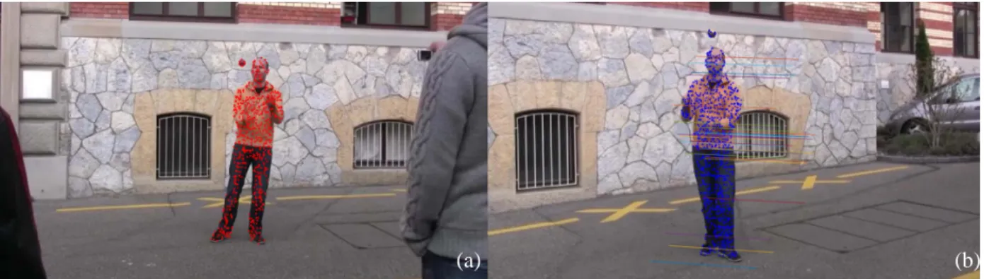
with low color consistency. (c) Segmented result. . . 35 4.3 (a) Local features in reference image. (b) Corresponding points are found

along the epipolar lines in the second image. . . 37 4.4 Red stars: Feature point in reference frame. Blue stars: Matched feature points

in the target frame. Green circles: Points with highest NCC values. In (a), the point with the highest NCC value is actually the correct correspondence. However, in (b), the green circle is indicating the wrong match. The other

candidate is the correct correspondence and should be used for triangulation. . . 37 4.5 In (a), trajectories from wrong correspondences deviate away from the inlier

trajectories (outlined in blue). (b) The sorted pairwise distance array of all inliers has no abrupt gradient in the middle, sorted pairwise distance array of

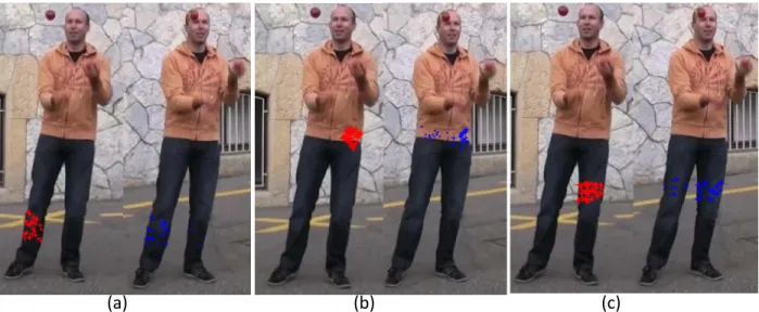
all trajectories will have those cutting edge when outlier trajectories are present. . . 41 4.6 Corresponding points in image pairs. Red dots (crosses): Feature (inlier)

points within one super-pixel in the reference frame. Blue dots (crosses): Correspondence (inlier) points found in the target frame. In (a), outliers on the left leg are detected because they located in different rigid parts. In (b), outliers on the right waist are removed because they are far away from majority of other trajectories. In (c), correct correspondences are the minority (there might be repetitive correspondences in the target frame). The wrong correspondences

are removed by the depth constraints. . . 42 4.7 (a) show depth map generated from raw correspondences (Left) and the

cor-rected correspondences (Right). (b)Average correspondences with different

offsets(red curve), the green boundary should the plus minus standard deviation. . . 43 4.8 Accuracy of our synchronization estimation across different datasets scenarios. . . 45 4.9 Results of corrected point cloud on the CMU dataset. Left: Blue 3D points

de-pict the originally reconstructed 3D points from initial correspondences, while red points denote the 3D points obtained through corrected correspondences. Left middle: Corresponding reference image. Right center: A side view of the

same structure. Right: Accuracy for both original and corrected point sets. . . 46 4.10 Qualitative results illustrating the effectiveness of our correspondence

5.1 Example time-lapse image of the Coliseum, the top image is automatically generated by our method, and the bottom is manually made by a photographer

(courtesy of Richard Silver). . . 49 5.2 Framework of our method. Given an input imageI, our method determines an

appearance neighborhoodNGIST(I)within a photo collection. We identify two

extremum elements ofI− ∈ NGIST(I)and I

+_N

GIST(I)to determine a path

within an appearance similarity graph, which corresponds to image sequence used for mosaic integration. We perform robust homography-based region warping to aggregate a mosaic. Finally, we transfer color from the mosaic into

our reference image. . . 50 5.3 Sky/building segmentation. (a) Original images, (b) Foreground mask, (c)

Background mask, (d) Sky segmentation. . . 53 5.4 Motivation for robust homography chains. (left) The reliability of direct

pair-wise homography estimation of an entire image sequence to a single reference image is not uniform across the sequence. Moreover, neighboring images may exhibit drastic appearance variation (especially at night), hindering di-rect homography chains. Green lines depict RANSAC inlier matches. (right) Schematic representation of (1) direct pairwise estimation, (2) direct

homogra-phy chains , and (3) our proposed bridge-based homograhomogra-phy estimation. . . 55 5.5 Mitigation of mosaicing artifacts. (a) Input reference image (b)

Homography-based image stitching (red rectangles highlight alignment problems). (c) SIFT-flow dense registration refinement partially resolves alignment issues, at the expense of small-scale structure aberrations (highlighted green boxes) (d)

Output image after transfering color from the mosaic to the reference image. . . 56 5.6 Sky reordering. Top: mosaics before reordering, red rectangles highlight

the inconsistent stripes. Bottom: reordered mosaics, the sky appearance

inconsistencies are mitigated. . . 59 5.7 Comparative results for baseline color transfer methods. Column (d) is

gener-ated by our color transfer method, refer to the text for specification of baselines. . . 62 5.8 Illumination mosaics for eight downloaded datasets. . . 63 5.9 Failed cases for our method. Artifacts appear mainly on the domes and round

6.1 MoFlow Network. In this example network, three input images are concate-nated as input for encoder network, the decoder network output three motion flows. Pixels of input image 3 are borrowed with learned motion flows to synthesize image in future timesteps so as to minimize the pixel reconstruction errors. The network iteratively borrows pixels from synthesized images to

generate future images. . . 68 6.2 (a)(b) Pose estimation results for images within a motion sequence. (c)

Com-puted motion flow with method (Beier and Neely, 1992). . . 71 6.3 Between left and right image, endpoints of line segmentM N are changed to

M0N0. . . 72 6.4 PoseFlow network. Left part of the network output pixel-wise predictions

of motion flow magnitude, and the right part is a fully connected network

predicting the future sparse poses that are densified into directional flow fields. . . 74 6.5 Two testing sequences forHuman3.6mdataset, compare results generated by

SIG92,ECCV16,MoFlowNetandPoseFlowNet. . . 77 6.6 Testing sequences for Spritesdataset (Row A: input frames, row B: ground

truth output frames), and compare results generated by ECCV16 (row C) and

MoFlowNet (row D). . . 78 6.7 Motion flow prediction evaluation (A: input image, B: next frame, C: Flow by

(Walker et al., 2015), D: Flow by PoseFlowNet, E: Groundtruth flow). . . 80 6.8 One sample test sequence for Human3.6M dataset (Row A: input frames, row

B: ground truth output frames), and compare results generated PoseFlowNet

LIST OF ABBREVIATIONS

MRF Markov Random Field

NCC Normalized cross correlation NRSFM Non-rigid structure from motion RANSAC Random sample consensus SfM Structure from motion

CHAPTER 1: INTRODUCTION

Our living environment is vibrant and intriguing because of dynamism. At a large scale, the Earth itself rotates in the space, creating days and nights in a perpetual flow. At scales visible to humans, we see water flowing down from the top of mountains, a juggler performing in the market, and billboards flashing at night. The world is constantly transient, persistent only in small moments, and we watch our seemingly static selves and creations change with time.

Visual perception is an important component in the human perception of time, and visual representations are therefore one of the most effective ways to record and convey the dynamic world we inhabit. In ancient times, people used carvings or paintings to express what they saw; art and history have always been deeply intertwined. In the last two centuries, film and video introduced increasingly authentic means for documenting the human experience. In the present age, the wide-spread availability of digital cameras, along with the existence of social media websites like Facebook, Snapchat, and Twitter, has enabled ubiquitous capture and sharing of the visual world. The growth of imagery in the Internet Age is overwhelmingly prolific. And here, the excitement of dynamism rises again: As we approach a near-constant, near-global capture of our world, how can we best represent the moments in which we live and the experiences we have today? Answering this question is a major sub-focus in the vast, ever-expanding field of computer vision.

et al., 2015); and high-quality motion capture applications rely on many synchronized video streams (Kanade et al., 1997; Joo et al., 2015). These creations, in turn, are widely adapted in applications like virtual tourism, virtual reality, autonomous driving, and special effects for movies.

However, the authentic representation of dynamic elements in our 3D world has yet to be completely attained, especially for the uncontrolled capture scenarios found in Internet-scale data. To bridge the gap in dynamic object representation from uncontrolled imagery, we explore research in two aspects: dynamic 3D reconstruction and dynamic view synthesis of scene elements.

Regarding 3D reconstruction, state-of-the-art crowd-sourced 3D reconstruction systems employ structure from motion (SfM) techniques that leverage large-scale imaging redundancy in order to generate photo-realistic models of scenes of interest. SfM (Frahm et al., 2010; Snavely et al., 2006; Zheng and Wu, 2015; Sch¨onberger and Frahm, 2016; Heinly et al., 2015) is the process by which the 3D geometry (structure) of a scene is recovered via a set of images taken from different viewpoints (which constitute camera motion). The estimated 3D models reliably depict both the shape and appearance of the captured environment under the joint assumptions of shape constancy and appearance congruency, both of which are commonly associated with static structures. Accordingly, the resulting 3D models are unable to robustly capture dynamic scene elements not in compliance with the aforementioned assumptions. Applying SfM to dynamic objects requires two methodological considerations: how to determine correspondences between images given that the object’s appearance may have changed, and how to model changes in the object’s geometry, position, or pose.

In a dynamic reconstruction framework, dynamic scene elements can be determined through the observation of visual motion. Nelson and Polana (Nelson and Polana, 1992) categorized visual motion into three classes: activities, motion events, and dynamic (temporal) texture change.

Activities, such as walking or juggling, are defined as motion patterns that are periodic in time;

criterion to categorize dynamic objects is whether the shapes or texture of the objects change, which classifies them into shape-deforming objects (Dynamic Shapes) and shape-constant objects with temporal appearance change (Dynamic Textures).

To reconstruct the 3D shape of dynamic textures, the geometry of those scene elements having time-varying appearance (e.g., active billboards, bodies of water, or building facades under varying illumination conditions) can be approximated by a single surface; in this thesis, a completely data-driven method that does not impose geometric or shape priors is proposed.

For objects having time-varying shape, several methods (Jiang et al., 2012; Joo et al., 2014, 2015; Mustafa et al., 2015; Zheng et al., 2015a, 2017; Russell et al., 2014; Garg et al., 2013) have been introduced over the last few years, with most of them assuming multi-view synchronized video sequences within controlled environments. Reconstruction with unsynchronized data captured in general scenes, such as multiple individuals filming a concert, is an unsolved problem that I tackle in this thesis. Taking as input a pair of unsynchronized video streams of the same dynamic scene, the method outputs a dense point cloud corresponding to the evolving shape of the commonly observed dynamic foreground. In addition to the 3D structures, the method estimates the temporal offset of the input pair of video streams, assuming a known frame-rate ratio between them.

First, considering the problem of modeling dynamic scene illumination, Internet photo-collections provide vast samples in the space of possible viewpoints and appearance configurations available for a given scene. Such images could be utilized to visualize the appearance change of a single viewpoint within a given time range. Here, we propose a method for augmenting a static image with the range of scene illuminations found in an Internet photo-collection, in a method combining geometry and appearance information.

Second, image-based motion prediction aims to generate plausible visualizations of the temporal evolution of dynamic scene elements. In addition to view synthesis, this problem is closely related to the problem of motion field estimation. Motion field estimation strives to determine dense pixel correspondences among a pair of image observations of a common scene. Given an input image and a motion field, it is straightforward to synthesize a novel image by simply locally shifting the image according to the 2D field. Conversely, given an input image and a synthesized image, there exists an abundance of methods to estimate the motion field. Inspired by the pioneer work of appearance flow network (Zhou et al., 2016), we propose to implicitly learn motion flow within visual prediction neural networks, which has the potential to generate images with more crisp textures than image prediction approaches.

1.1 Thesis Statement

1.2 Outline of Contributions

This dissertation contributes significantly to advance the state-of-the-art techniques for the problems of 3D reconstruction of dynamic objects and data driven dynamic view synthesis, and it builds on our published works (Ji et al., 2014, 2016, 2015; Radenovi´c et al., 2016; Ji et al., 2017). 3D Reconstruction of Dynamic Textures: Chapter 3 aims for a more complete and realistic 3D

scene representations by addressing the 3D modeling of dynamic scene elements within the context of crowd-sourced input imagery. The input data to my proposed framework encompasses both online image and video collections capturing a common scene. Sparse reconstruction is first performed for the rigid scene elements. Then, video collection data is analyzed to reap video segments amenable for 1) registration to the existing rigid model and 2) coarse identification of dynamic scene elements.

The proposed method adopts these coarse estimates, along with the knowledge of the sparse rigid 3D structure, to pose the segmentation of dynamic elements within an image as a global two-label optimization problem. The attained dynamic region masks are subsequently fused through shape-from-silhouette techniques in order to generate an initial 3D shape estimate from the input videos. The preliminary 3D shape is then back projected to the original photo-collection imagery, and all image labelings are then recomputed and fused to generate an updated 3D shape. This process is iterated until convergence of the output photo-collection imagery segmentation process.

the spatio-temporal domain. In this respect, the main challenges are 1) finding a common temporal reference frame across independent video captures, and 2) meaningfully propagating temporally varying photo-consistency estimates across videos.

In this work, we propose to address both of these challenges by enforcing the geometric con-sistency of optical flow measurements across spatially registered video segments. Moreover, the proposed approach builds on the thesis that maximally consistent geometry is obtained with minimal temporal alignment error, and vice versa. Towards this end, we posit that it is possible to recover the spatio-temporal overlap of two image sequences by maximizing the set of consistent spatio-temporal correspondences among the two video segments.

Appearance Analysis of Scenes Under Different Illuminations: Chapter 5 strives to address the organization and characterization of the image space by exploring the link between time-lapse photography and crowd-sourced imagery. Time-time-lapse photography strives to depict the evolution of a given scene as observed under varying image capture conditions. While the aggregation of a sequence of images into a video may be the most straightforward visualization for time-lapse photography, the integration of multiple images in the form of a mosaic provides a descriptive 2D representation of the observed scene’s temporal variability. The problem of mosaic construction can be abstracted as a three-stage process of image registration, alignment, and aggregation. However, the representation of the appearance dynamics introduces the qualitative challenge of producing an aggregate mosaic that is both coherent with the original scene content and descriptive of the fine-scale appearance variations across time. We address these challenges by exploring the spectrum of capture variability available in Internet photo-collections and propose a novel framework to obtain illumination mosaics.

encoder-decoder networks has been widely adopted in both kinds of methods. Pixel prediction via these networks has been shown to suffer from blurry outputs, since images are generated from scratch and there is no explicit enforcement of visual coherency. However, crisp details can be achieved by transferring pixels from the input image through trajectory prediction, but this requires pre-computed motion fields for training. To synthesize realistic movement of objects under weaker supervision, we propose a novel network structure, inspired by appearance flow networks (Zhou et al., 2016). Motion priors (sparse joint positions of rigid body movements) are further incorporated to enable more efficient appearance synthesis.

CHAPTER 2: RELATED WORK

Related to the problem of dynamic 3D reconstruction and dynamic view synthesis, many approaches have been proposed to address issues relating to them. This section outlines several related efforts in each of these areas.

2.0.1 3D Reconstruction of Dynamic Objects

For static environments, very robust SfM systems (Agarwal et al., 2012; Heinly et al., 2015; Wu, 2013) and multi-view stereo (MVS) approaches (Furukawa and Ponce, 2010; Sch¨onberger et al., 2016; Zheng et al., 2014) have shown much success in recovering scene geometry with high accuracy on a large variety of datasets. Modeling non-static objects with those frameworks, however, is considerably more difficult because the assumptions driving correspondence detection and 3D point triangulation in rigid scenarios cannot be directly applied to moving objects. To address these challenges, a wide array of dynamic scene reconstruction techniques have been introduced in the computer vision literature, in capture situations that are controlled or uncontrolled, synchronized or unsynchronized, single-view or multi-view, and model-based or model-free.

multi-camera system specifically tailored for dynamic object capture. These works, and others (Martin and Daniel, 2013; Oswald et al., 2014; Djelouah et al., 2015; Letouzey and Boyer, 2012; Wu et al., 2011; Guan et al., 2010; Cagniart et al., 2010), clearly indicate the strong potential for non-rigid reconstruction in controlled capture scenarios, and they highlight in particular the usefulness of multiple synchronized video streams toward this end.

3D reconstruction of dynamic scenes in uncontrolled environment is a challenging problem for computer vision research. Several systems have been developed for building multiview dynamic outdoor scenes. Jiang et al. (Jiang et al., 2012) and Taneja et. al. (Taneja et al., 2010) propose probabilistic frameworks to model outdoor scenes with handheld synchronized cameras. By incorporating depth consistency within depth maps and images, these frameworks could obtain smooth depth maps and 3D surfaces. Pollefeys et al. (Pollefeys et al., 2007) built a large scale 3D reconstruction system that combines GPS and inertial info with videos to generate a 3D mesh in urban scenes. Again, these systems all rely on a set of pre-calibrated or synchronized cameras. In this thesis, we propose two frameworks to recover 3D geometry of dynamic scene elements captured in uncontrolled environments, with Internet downloaded imagery which extensively vary in environment and camera parameters and hand-held unsynchronized video streams respectively.

further asserts that both outlier correspondences and reduced/small temporal overlap will hinder the accuracy of the temporal alignment.

Besides of Zhenget al. (Zheng et al., 2015a, 2017), multi-view geometric reasoning has been employed for the problem of video synchronization. For example, Bashaet al. (Basha et al., 2012, 2013) proposed methods for computing partial orderings for a subset of images by analyzing the movement of dynamic objects in the images. There, dynamic objects are assumed to move closely along a straight line within a short time period, and video frames are ordered to form a consistent motion model. Tuytelaars and Gool (Tuytelaars and Gool, 2004) proposed a method for automatically synchronizing two video sequences of the same event. They do not enforce any constraints on the scene or cameras, but rather rely on validating the rigidity of at least five non-rigidly moving points among the video sequences, matched and tracked throughout the two sequences. In (Wolf and Zomet, 2006), Wolf and Zomet propose a strategy that builds on the idea that every 3D point tracked in one sequence results from a linear combination of the 3D points tracked in the other sequence. This approach works with articulated objects, but requires that the cameras are static or moving jointly. Finally, Pundik and Moses (Pundik and Moses, 2010) introduced a novel formulation of low-level temporal signals computed from epipolar lines. The spatial matching of two such temporal signals is given by the fundamental matrix relating each pair of images, without requiring pixel-wise correspondences. In this thesis, a method computing spatio-temporal consistent correspondences are proposed to model rigid body movements, which could also be adopted to align unsynchronized video streams.

Single-view video capture can be considered as a dynamic reconstruction scenario inherently lacking the benefits of multi-view synchronization. On this front, the monocular method of Russell

our method utilizes perspective camera model, which is not recoverable using monocular input alone.

more accurate model by accumulating view ray hits for voxels instead of simply carving. In order to address problems like occlusion inference and multi objects modeling, Guan et al.(Guan et al., 2008) further propose a Bayesian fusion framework.

While previous methods discussed in this section mostly belong to model-free methods, model based methods are widely adopted to recover the dynamic 3D geometry. Most of these methods require extra priors on the shape or camera matrices to resolve the ambiguities. (Park et al., 2010; Akhter et al., 2011; Bartoli et al., 2008) assume temporal smoothness by synthesizing motion trajectories with a pre-defined trajectory basis. (C. Bregler and Biermann, 2010; Garg et al., 2013; Zheng et al., 2015a, 2017) assume the 3D shape at any frame can be expressed as a linear combination of an unknown low-rank shape basis governed by time-varying coefficients. To reduce the problem complexity, (C. Bregler and Biermann, 2010; Garg et al., 2013) assume orthogonal camera projection to the image planes instead of projective projections. The methods proposed in this thesis require no shape priors and simpler camera model, instead we adopt motion priors inspired by rigidity.

2.0.2 Appearance Analysis and Mosaics

In this thesis, we present a method to automatically generate image sequences showing smooth illumination change from night-time to day-time (shown in Fig. 5.1). There exists a large body of research on modeling the temporal order of images based on appearance. Wanget al. (Wang et al., 2006) propose low-dimensional manifolds to model the gradual appearance change of materials. In order to find smooth transitions between images of faces, Shlizerman et al. (Kemelmacher-Shlizerman et al., 2011) build a graph with faces as nodes and similarities as edges, and solve for walks and shortest paths on this graph. For natural scenes like the appearance of the sky, Tao

image segmentation and global color transfer. Instead of the sky, we focus on generating the temporal change of more general scenes and adopt local color transfer techniques to better portray the color transition. Schindler and Dellaert (Schindler and Dellaert, 2007) propose a constraint-satisfaction method for determining the temporal ordering of images based on visibility reasoning of reconstructed 3D points. They further present a generalized framework (Schindler and Dellaert, 2010) for estimating temporal variables in SFM problems and obtaining the temporal order of images. Their methods work for images taken over decades of time. Palermoet al. (Palermo et al., 2012) extract features that are temporally discriminative and show outstanding results in temporal classification of historical images. Kimet al. (Kim et al., 2010) propose a non-parametric approach for modeling and analysis of the topical evolution for Internet images with time stamps. Jacobs

et al. (Jacobs et al., 2007) created a large dataset of over 500 static web-cameras around the world and propose a method to analyze consistent temporal variations in these scenes. Our proposed method mines unorganized crowd-sourced data to identify a suitable visual datum and generate photo sequences from day to night. There has been tremendous progress in modeling unordered Internet image collections (Frahm et al., 2010; Agarwal et al., 2011; Heinly et al., 2015; Schonberger et al., 2015). The work of Snavelyet al. (Snavely et al., 2008, 2006) enabled the spatially smooth traversal from Internet images of landmark scenes. Leeet al. (Lee et al., 2000) propose a system to “rephotograph” historical photographs. Xuet al. (Xu et al., 2008) use collections of images to infer the motion cycle of animals. Hays and Efros (Hays and Efros, 2007) propose an image completion algorithm which fills in empty areas by finding similar image regions in a large dataset.

alignment model that combines homography and content-preserving warping to provide flexibility for handling parallax. However, this method is not designed to align image sequences and did not show results to align images with very different illuminations.

2.0.3 View Synthesis and Visual Predictions

Long range motion flow. Optical flow estimation among successive frames is mainly used to

generate motion flows (Black and Anandan, 1991; Elad and Feuer, 1998; Shi and Malik, 1998). Broxet al. (Brox et al., 2014; Papenberg et al., 2006) estimate optical flows simultaneously within multiple frames by adopting robust spatio-temporal regularization. Wills and Belongie (Wills and Belongie, 2004) estimate dense correspondences of image pairs using a layered representation initialized with sparse feature correspondences. Irani (Irani, 1999) describes linear subspace constraints for flow across multiple frames. Brand (Brand, 2001) applies a similar approach to non-rigid scenes. Sand and Teller (Peter Sand, 2006) propose to represent video motion using a set of particles, which are optimized by measuring point-based matching along the particle trajectories and distortion between the particles.

Future prediction. Future prediction has been used in various tasks such as estimating the

future trajectories of cars (Walker et al., 2014), pedestrians (Kitani et al., 2012), or general objects (Yuen and Torralba, 2010) in images or videos. Given an observed image or a short video sequence, models have been proposed to predict a future motion field (Liu et al., 2009b; Pintea et al., 2014; Walker et al., 2015, 2016). Zhou and Berg (Zhou and Berg, 2015) frames the prediction problem as a binary selection task to determine the temporal sequence of two video clips. (Vondrick et al., 2015) trains a deep network to predict visual representations of future images with large amounts of unlabeled video data from the Internet.

input stereo pair. Dosovitiskiyet al. (Dosovitskiy et al., 2015) learned a generative CNN model to hallucinate chairs with respected to given input graphics codes i.e. identity, pose, and lighting. Inspired by this paper, Tatarchenkoet al. (Tatarchenko et al., 2016) and Yanget al. (Yang et al., 2015) instead adopt an encoder-decoder network to implicitly learn graphics code from training image pairs or sequences. Tatarchenkoet al. (Tatarchenko et al., 2016) proposed an approach to predict images and silhouette masks without explicit decoupling of identity and pose. Yanget al. (Yang et al., 2015) applied input transformation to the learned pose units of source images to obtain desired target images, and apply a recurrent network to enable synthesizing sequences with large viewpoint difference.

CHAPTER 3: 3D RECONSTRUCTION OF DYNAMIC TEXTURES IN CROWD SOURCED DATA

3.1 Introduction

State of the art crowd sourced 3D reconstruction systems deploy structure from motion (SfM) techniques leveraging large scale imaging redundancy in order to generate photo-realistic models of scenes of interest. The estimated 3D models reliably depict both the shape and appearance of the captured environment under the joint assumptions of shape constancy and appearance congruency, commonly associated with static structures. Accordingly, the attained 3D models are unable to robustly capture dynamic scene elements not in compliance with the aforementioned assumptions. In this work, we strive to estimate more complete and realistic 3D scene representations by addressing the 3D modeling of dynamic scene elements within the context of crowd sourced input imagery.

First, we briefly give an overview of the functionality of our processing pipeline. The input data to our framework encompasses both online image and video collections capturing a common scene. We initially leverage photo-collection data to perform sparse reconstruction of the rigid scene elements. Then, the video collection is analyzed to reap video segments amenable for 1) registration to our existing rigid model and 2) coarse identification of dynamic scene elements. We use these coarse estimates, along with the knowledge of our sparse rigid 3D structure to pose the segmentation of dynamic elements within an image as a global two-label optimization problem. The attained dynamic region masks are subsequently fused through shape-from-silhouette techniques in order to generate an initial 3D shape estimate from the input videos. The preliminary 3D shape is then back projected to the original photo-collection imagery, all image labelings are recomputed and then fused to generate an updated 3D shape. This process is iterated until convergence of the output photo-collection imagery segmentation process. Figure 3.1 depicts an overview of the proposed pipeline.

Online image collection

Online video collection Frame selection

Structure from motion Dynamic 

Content Analysis

Fore/background Graph‐cut Shape‐from‐silhouettes

Not Converge

Proje ct   model   to   imag e s Image  dynamic prior Image 

static prior Video

static prior Video 

dynamic prior

Converge

Figure 3.1: Workflow overview of the proposed framework.

model surfaces having time varying appearance. The remainder of this chapter describes the design choices and implementation details of different modules comprising our dynamic scene content modeling pipeline.

3.2 Initial Model Generation

3.2.1 Static Reconstruction from Photo Collections

The first step in our pipeline is to build a preliminary 3D model of the environment using photo-collection imagery. To this end we perform keyword and location based queries to photo sharing websites Flickr & Panoramio. We perform GIST (Oliva, 2005) based K-means clustering to attain a reduced set images on which to perform exhaustive geometric verification. We take the largest connected component in the resulting camera graph, consisting of pairwise registered cluster centers, as our initial sparse model and perform intra-cluster geometric verification to densify the camera graph. The final set of images is fed to the publicly available VisualSfM module to attain a final sparse reconstruction. The motivation for using VisualSfM is the availability for direct comparison against two input compatible surface reconstruction modules PMVS2(Furukawa and Ponce, 2010) by Furukawa & Ponce and CMPMVS(Jancosek and Pajdla, 2011) by Jancosek & Pajdla. Once a static sparse model is attained the focus shifts to identifying additional video imagery enabling the identification and modeling of dynamic scene content.

3.2.2 Coarse Dynamic Textures Priors from Video

Video Frame Registration. We temporally sample each video at a 1/50 ratio to obtain a reduced set of video frames for analysis. For illustration, a set of 500 videos generated little over 80K frame samples. We introduce into the video frame set a random subset of 30% of the registered cameras from the rigid scene modeling. We again perform GIST based clustering on the augmented image set and re-run intra cluster geometric verification to identify registered video frames. In principle, the entire process can be performed directly on the joint set of input photo-collection images and sampled video frames. However, we found the implemented two stage image and video registration to provide more robust performance and increased video frame registration.

Video Sub-sequence Selection. Given a reduced set of registered video frames we want to select compact frame sub-sequences having reduced camera motion in order to simplify the detection of dynamic scene content. Namely, we compute the HOG descriptor for the frames immediately preceding and following a registered video frame in the original sequence. We count the number of neighboring frames having an NCC value in the range(0.9,1)w.r.t. the registered frame and keep those sequences having cardinality above a given thresholdτseq len. We favor such

image content based approach instead of pair-wise camera motion estimation due to the difficulty in defining suitable capture dependent thresholds (i.e. camera motion, lighting changes, varying zoom, etc.). Discarding fully correlated (i.e. NNC=1) pairwise measurements enables the elimination of duplicates. Moreover, we found measuring the NCC over the HOG descriptors to be robust against abrupt dynamic texture variation as long such changes were restricted to reduced image regions. Figure 3.2 describes the selection thresholds utilized for subsequence detection.

Figure 3.2: Keyframe selection for an input video. The plot shows the frame number count vs the NCC similarity of each frame’s HOG descriptor. Red boxes indicate selected video fragments centered on sampled frames. Keyframe selection is a function of the plot density at the upper end of the NNC values.

for an input image of VGA resolutions. We sort the connected component of the binary output image w.r.t. their area and eliminate all individual components at the bottom 10% of total image area (shown in Figure 3.3).

Figure 3.3: Dynamic content priors from video fragments. Left to right: (a) Reference frame (b) Accumulated frame differencing (c) Result after post processing.

3.2.3 Coarse Static Background Priors from Video Frames

using the complement of the precomputed dynamic texture mask for a given video frame, we strive to deploy a more data-driven approach. To this end we analyze the sparse feature similarity among the reference frame and one of its immediate neighbors. We retrieve the set of putative SIFT matches previously used for homography based stabilization of the video sequence and perform RANSAC based epipolar geometry estimation. We consider the attained set of inlier image features in the reference videoframe as a sparse sample of the observed static structure. To mitigate spurious dynamic features being registered due to low frequency appearance variations, we exclude from this set any features contained within the regions described by dynamic texture mask. From the final image feature set we compute the concave hull and use the attained 2D polygon as an area based prior for static scene content(shown in Figure 3.4).

Figure 3.4: Static content prior from video fragments. First and third columns depict SIFT features matches among neighboring frames as red dots. Second and fourth columns depict the concave hull defined by detected features not overlapping with the existing dynamic content prior.

3.2.4 Graph-cut based dynamic texture refinement

Once a preliminary set of segmentation masks for static and dynamic object regions are attained, they are refined trough a two label (e.g. foreground/background) graph-cut labeling optimization framework. We will denote static structure as background and dynamic content as foreground. The optimization problem in Graphcut is defined as:

minE(f) = X

u∈U

DU(fu) +

X

u,v∈N

wherefu, fv ∈ {0,1}are the labels for pixelsuandv,N is the set of neighboring pixels foruand

U denotes the set of all the pixels with unknown labels. Similarly to the work of Jiangyu (Liu et al., 2009a), we use a Gaussian mixture model to compute the foreground/background membership probabilities of a pixel. Hence, the smoothness term is defined to be:

Vu,v(fu, fv) =|fu−fv|exp(−β(Iu−Iv)2), (3.2)

whereIu, Ivdenote the RGB values of pixelsuandv, whileβ= (2h(Iu−Iv)2i)−1, forh·idenoting

the expectation over an image sample. Conversely, the data term is defined as:

Du(fu) = log

p(fu = 1)

p(fu = 0)

, (3.3)

p(fu = 1) =p(Iu|λ1) = P_iM₌₁ωi1g(Iu|µi1,Σi1)

p(fu = 0) =p(Iu|λ0) =

PM

i=1ωi0g(Iu|µi0,Σi0) λ1|0 ={ωi1|0, µi1|0,Σi1|0}, i∈ {1,2, ..., M}

andg(Iu|µi,Σi)belongs to a mixture-of-gaussian model usingM = 3, and we assume the labels

for fore/background are 1/0.

Figure 3.5 exemplifies the result of graph-cut segmentation. Moreover, the output regions categorized as foreground (i.e. dynamic content)

3.2.5 Shape from silhouettes

Figure 3.5: Graphh-cut label refinement. First and third rows depict (alternatively from left to right) single image dynamic and static content priors. Second and fourth rows depict the outputs of the label optimization, where green regions are dynamic textures.

estimate, to deploy a 3D fusion method estimating a volumetric shape representation in accordance to the steps described in Algorithm 1.

Algorithm 1:SHAPE FROM SILHOUETTES FUSION

Input: Sets of camera poses{_Ci}and corresponding foreground silhouettes{Mi}, where

i∈[1,· · · , N], 3D occupancy gridO, thresholdθ1 Output: Labeled 3D occupancy gridV

1 Set allO(x, y, z) = 0

2 fori∈[1, N]do

3 forpixelM_ij ∈ {_Mi}do

4 Find all voxelsOx,y,z,{x, y, z} ∈O1 ⊂O ,P roji(O1) = Mij

5 O₁ ←O₁+ 1

Algorithm 2:SHAPE FROM SILHOUETTES FUSION

Input: Sets of camera poses{_Ci}and corresponding foreground silhouettes{Mi}and

background silhouettes{_M0_i}, wherei∈[1,· · · , N], 3D occupancy gridO, threshold θ1, θ2

Output: Labeled 3D occupancy gridV

1 Set allO(x, y, z) = 0

2 fori∈[1, N]do

3 forpixelM_ij ∈ {_Mi}do

4 Find all voxelsOx,y,z,{x, y, z} ∈O1 ⊂O ,P roji(O1) = Mij

5 O₁ ←O₁+ 1

6 V =F ind({x, y, z}|Ox,y,z > θ1),{x, y, z} ∈V ⊂O

7 Set allV(x, y, z) = 0

8 fori∈[1, N]do

9 forpixelM0_ij ∈ {_M0_i}do

10 Find all voxelsVx,y,z,{x, y, z} ∈V1 ⊂V ,P roji(V1) =Mij0

11 V₁ ←V₁+ 1

12 V =F ind({x, y, z}|V_x,y,z < θ₂),{x, y, z} ∈V 13 Label voxels inV as occupied.

3.3 Closed Loop 3D Shape Refinement

The preceding section described a video based approximation of the observed shape of dynamic texture within the scene. The motivation for exclusively using video keyframes until now has been the lack of a mechanism to estimate dynamic texture prior for static images. In this section, we describe an iterative mechanism to effectively transfer the labelings attained from video sequences to the available photo-collection imagery. Such label transferring will enable us to leverage and augmented imagery dataset offering 1) increased robustness through additional redundancy and viewpoint diversity as well as 2) increased level of detail afforded by larger available imaging resolutions.

3.3.1 Geometry based Video to Image Label Transfer

1. Generate static background priors for each image.

2. Project the preliminary 3D shape model to all registered images and use its silhouette as a dynamic foreground prior for each image.

3. Execute graph-cut based label optimization

4. Generate an updated 3D model using the shape from silhouettes module.

Steps 2 to 4 in the above method will iterate until convergence of the dynamic foreground prior mask. Note that in such a framework the static background priors are kept constant while the dynamic texture content is a function of an evolving 3D shape. In general, the preliminary model attained from videos sequences may suffer from a variability viewpoint coverage or be sensitive to errors in our video based video segmentation estimates. While the former may either under-constrain or bias the attained 3D shape, the latter may arbitrarily corrupt the estimate. Both of these challenges are addressed through the additional sampling redundancy afforded by image photo-collections. The remaining challenges consist then in robustly defining static content priors for single images and adapting the shape estimation framework to adequately handle the heterogeneous additional imaging data.

3.3.2 Mitigating Dynamic Texture in SfM Estimates

The variability in the temporal behavior and extent of dynamic textures may enable its spurious inclusion within SfM estimates. Namely, it is possible for changes in appearance to manifest themselves at time scales larger than those encompassed through short video subsequences or to present periodic behavior that would enable feature correspondence across multiple unsynchronized image captures. We evaluate the appearance variability of sparse reconstructed features across the imaging dataset to classify them having either persistent or sporadic color.

ocean, flashing letters on a billboard etc. The existence of reconstructed features within a dynamic texture obeys mainly to the transient nature of their appearance. That is, while such appearance is observable at multiple different times, the same structure element may alternatively display appearance independent of the one used for matching.

Moreover, according to Lambert’s cosine law, if the colors of a static structure remains constant, the observed pixels are linearly correlated to intensity of the incoming light, as described by

ID =L·NCIL=CILcosα, (3.4)

WhereL and Nare the normalized incoming light direction and the normalized normal for 3D object,CandILthe color of the model and the intensity of incoming light respectively, making the

reflection colorID a linear function ofIL(with slopecosα). Given that robust features (e.g. SIFT,

SURF) enable the robust detection of features even in the presence of such lighting variations, we can generally expect the color variability of a static feature to comply with such linear behavior. Based on this assumption, we propose a simple method for consistency detection. First we re-project each reconstructed feature to all cameras observing the same structure and record the observed RGB pixel color. Note we re-project to all cameras where the feature fall within the viewing frustum, not just those cameras where the feature was detected. We perform RANSAC based line fitting on the set of measured RGB values to determine the inlier ratiofor a pre-specified distanced1 = 0.08in the RGB unit color cube. We consider any feature with an estimated inlier ratio below 0.6 to have sporadic color. Figure 3.6 shows the results running our method on a billboard dataset. Moreover, the set of features classified as having sporadic color will be subsequently used to filter sparse SfM estimates corresponding to static structure.

3.3.3 Building a Static Background Prior for Single Images

Figure 3.6: Identification of dynamic textures within existing SfM estimates.Top Row: birds-eye and fontal view of estimated sparse structure for Piccadilly Circus. Blue dots are 3D features with persitent color across the dataset. Red dots are 3D features determined to have sporadic color. The bottom row shows sample images in the dataset. We associate color persistance with predominantly linear variation in the RGB space.

3.3.4 Mitigating of Non-uniform Spatial Sampling

In order to generate accurate 3D shape models of dynamic scene elements through space carving methods wide spatial coverage of cameras is a requisite. In fact, this is the motivation of using photo-collection images. However, the availability of abundant images also presents challenges when said imagery is not uniformly distributed within the scene. Namely, we require a large number of viewing rays tangent to the shape’s surface in order for the estimated visual hull to accurately approximate the observed surface. Moreover, our basic shape from silhouettes method will favor the identification of commonly observed image regions. For example, to accurately estimate the shape for the Piccadilly circus billboard (which is a round rectangled shape), we require cameras located in a range of nearly270◦. Figure 3.7 shows the reconstruction of Piccadilly circus using 5800 iconic images(from more than 60,000 images). We can see the camera distribution is not uniform providing scarce coverage of the tangent views of the billboard. Densely distributed cameras dilute the weights of sparsely distributed cameras in (Algorithm 2). And the generated 3D shapes will deform towards the direction of densely distributed cameras (shown in Figure 3.7(c)). In order to deal with the uncontrolled viewpoint distribution we deploy a weighting mechanism (Algorithm 3) within our image base shape from silhouettes framework. The idea is to reduce relative weights of densely distributed cameras. To obtains new set of weights for cameras, we compute viewing ray angle between reference camera and other cameras, generating a histogram for the angles and set the weights of cameras located in each bin with the inverse of camera numbers. After applying weighting strategy, the computed models are visually more natural.

(a) (b) (c) (d)

Algorithm 3:camera weighting strategy

Input: A initial modelM0, camera centersCi, i∈[1,· · · , N], cameras field-of-view angles

fi, i∈[1,· · · , N]

Output: Space carving weightwi for each camera

1 fori∈[1,· · · , N]do

2 Direction vector of each camera centerv_i ←C_i−centroid(M₀) 3 Direction angle of each camera centera_i ←arccos_norm(vvi∗vN/2

i)norm(vN/2)

4 wi = 1

5 Discretize the direction angles into 5 bins histogram centered atB_j, j ∈[1,· · · ,5], with

frequencyHj, j ∈[1,· · · ,5]

6 fori∈[1,· · · , N]do

7 idx=f ind(j|B_j ≤a_i < B_j+1)

8 wi ←wi∗min(H)/Hidx

9 w_i ←w_i∗min(f)/f_i

3.4 Experiments

We downloaded 4 online datasets from the Internet, with videos attained from Youtube and images from Flickr. The statistics of our data associations are presented in Table 3.1. For all datasets, the set of registered images and the final sparse SfM was generated using visualSfM. Figure 3.9 shows our results combining PMVS quasi-dense model and our dynamic texture shape estimate.

Table 3.1: Composition of our downloaded crowd sourced datasets

Dataset Videos Keyframes Images Images

Downloaded Extracted Downloaded Registered

Trevi Fountain 481 68629 6000 810

Navagio Beach 300 45823 1000 520

Piccadilly Circus Billboard 460 75983 5000 496

Mooney Falls 200 17850 1000 723

Space carving result  (frontal  view)

Space carving result  (top view)

The efficacy of our weighted space carving method for photo collection imagery is illustrated for the Piccadilly Circus Billboard dataset in Figure 3.7 We can see in the absence of camera contribution weighting, the model will outstretch in the direction of greater camera density. The effect is effectively mitigated by our weighting approach. We also generate the textured 3D model and compare the results generated by the state-of-the-art method CMPMVS (Jancosek and Pajdla, 2011) (Fig. 3.9). For all the experiments, we use the same input dataset for comparison. Each dataset takes a approximately 24 hours of processing using both methods.

Figure 3.9: Top two rows: sample dataset imagery, respective outputs for PMVS, CMPMVS and our proposal. Bottom two rows: sample dataset imagery, respective outputs for PMVS and our proposal; CMPMVS failed to generate on the same input data.

approximation of the screen surface of an electronic tablet displaying dynamic texture(shown in Fig. 3.10). In practice, the inability to attain observations of the dynamic texture of a flat surface from completely oblique views yielded a piece-wise planar 3D surface with slight outside of plane protrusions. Nevertheless, our attained 3D model was amenable for video texture mapping yielding a realistic animation of the captured video.

Figure 3.10: From left to right: sample dataset imagery, respective outputs of PMVS, CMPMVS and our proposed method.

3.5 Conclusion

CHAPTER 4: SPATIO-TEMPORALLY CONSISTENT CORRESPONDENCE FOR DENSE DYNAMIC SCENE MODELING

4.1 Introduction

Dynamic 3D scene modeling addresses the estimation of time-varying geometry from input imagery. Existing motion capture techniques have typically addressed well-controlled capture scenarios, where aspects such as camera positioning, sensor synchronization, and favorable scene content (i.e.fiducial markers or “green screen” backgrounds) are either carefully designeda priori

or controlled online. Given the abundance of available crowd-sourced video content, there is grow-ing interest in estimatgrow-ing dynamic 3D representations from uncontrolled video capture. Whereas multi-camera static scene reconstruction methods leverage photoconsistency across spatially varying observations, their dynamic counterparts must address photoconsistency in the spatio-temporal do-main. In this respect, the main challenges are 1) finding a common temporal reference frame across independent video captures, and 2) meaningfully propagating temporally varying photo-consistency estimates across videos. These two correspondence problems – temporal correspondence search among unaligned video sequences and spatial correspondence for geometry estimation – must be solved jointly when performing dynamic 3D reconstruction on uncontrolled inputs.

Tracking

Ma

tc

hing

Trajectory  Triangulations

Reconstructed Points 

(Profile view) ConsistentGeneration Correspondence   Depth Map Generation 

Figure 4.1: Overview of the proposed approach for dense dynamic scene reconstruction from two input video streams.

In practice, our approach addresses the spatio-temporal two-view stereo problem. Taking as input two unsynchronized video streams of the same dynamic scene, our method outputs a dense point cloud corresponding to the evolving shape of the commonly observed dynamic foreground. In addition to outputting the observed 3D structure, we estimate the temporal offset of a pair of input video streams with a constant and known ratio between their frame rates. An overview of our framework is shown in Fig. 4.1. Our framework operates within local temporal windows in a strictly data-driven manner to leverage the low-level concepts of local rigidity and non-local geometric coherence for robust model-free structure estimation. We further illustrate how our local spatio-temporal assumptions can be built to successfully address problems of much larger scope, such as content-based video synchronization and object-level dense dynamic modeling.

4.2 Spatio-Temporal Correspondence Assessment

filtering mechanism, and 2) to provide a measure of local spatio-temporal consistency among video sub-sequences in terms of the size of the valid correspondence set. We explore both these interpretations within the context of video synchronization and dense dynamic surface modeling.

4.2.1 Notation

Let{I_i}and{I0_j}denote a pair of input image sequences, where1≤i≤M and1≤j ≤N are the single image indices. For each imageIk ∈ {Ii} ∪ {I

0

j}, we first obtain via

structure-from-motion (SfM) a corresponding camera projection matrix,P(Ik) =Kk[Rk| −RkCk], whereK,R,

andCrespectively denote the camera’s intrinsic parameter matrix, external rotation matrix, and 3D position. LetFij denote the fundamental matrix relating the camera poses for imagesIi andIj0.

Furthermore, letOiandOj0 denote optical flow fields for corresponding 2D points in consecutive

images (e.g.Ii → Ii+1 and Ij0 → I

0

j+1) in each of the two input sequences. Finally, letxip and

Xipdenote the 2D pixel position and the 3D world point, respectively, for pixelpin imageIi(and

similarlyx0_jpandX0_jpfor imageI0

j).

(a)(a) (b) (c)

Figure 4.2: (a) Background mask that has high color consistency. (b) Foreground mask with low color consistency. (c) Segmented result.

4.2.2 Pre-processing and Correspondence Formulation

methods (Wu et al., 2011) over the aggregated set of frames, producing a spatial registration of the individual images from each stream. Since the goal of this stage is simply image registration of the two sequences, the set of input images for SfM can be augmented with additional video streams or crowd-sourced imagery for higher-quality pose estimates; however, this is not necessarily required for our method to succeed.

Correspondence Search Space. Consider two temporally corresponding image frames Ii and

I0

j. For a given pixel positionxipcontained within the dynamic foreground mask of imageIi, we

can readily compute a correspondencex0_jp in imageI0

j by searching for the most photoconsistent

candidate along the epipolar lineFijxip. We can further reduce the candidate setΩ(xip,Fij)∈ Ij0

by only considering points along the epipolar line contained within the foreground mask ofI0

j.

In this manner, we have Ω(xip,Fij) = {x0jq | xipFijx0jq = 0}. Henceforth, we shall omit the

dependence on the pre-computed camera geometry and segmentation estimates from our notation, denoting the set of candidate matches for a given pixel asΩ(xip). We measure the NCC w.r.t. the

reference pixelxipusing15×15patches along the epipolar line, and all patches with a NCC value

greater than 0.8 are deemed potential correspondences. OnceΩ(xip)is determined, its elementsx0jq

are sorted in descending order of their photoconsistency value. Fig. 5.4 provides an example of our epipolar correspondence search for an image pair.

Frames

segmentation

(a) (b) (c)

(a) (b)

(a) (b)

Figure 4.3: (a) Local features in reference image. (b) Corresponding points are found along the epipolar lines in the second image.

(a) (b)

4.2.3 Assessment and Correction Mechanism

Based on the example shown in Fig. 5.4, we propose a method to discern wrong correspondences and correct them with alternative pixel matches. The steps of our method are as follows:

4.2.3.1 Step

¶

The set of 2D feature points {xip} and currently selected corresponding points {x0jq} are

updated with optical flow motion vectors computed between neighboring frames using the approach of Brox et al. (Brox et al., 2004). Thus we have{xi+1,p}={xi,p}+Oi and{x0j+1,q}={xjq}+O

0

j.

We select the video with the higher frame rate as the target sequence, which will be temporally sampled according to the frame rate ratioα among the sequences. The reference sequence will be used at its native frame rate. Hence, given a temporal window of W frames, the reference video frames and their features will be denoted, respectively, byIi and{xi,p}, where1≤i≤W,

denotes the frame index. Accordingly, the frames and features in the target video frames will be denoted byI0

j and{x

0

j+w∗α,q}, wherej corresponds to the temporal frame offset between the two

sequences, and 0 ≤ w < W. The size of the temporal window must strike a balance between building informative 3D tracks for spatial analysis and maintaining the reliability of the chain of estimated dense optical flows.

The initial set of correspondence estimates{xip},{x0jq}are temporally tracked through

succes-sive intra-sequence optical flow estimates, and their updated locations are then used for two-view 3D triangulation. Namely, for each pointxipselected at framep, we have a 3D trackTi ={Xiw}

comprised of1≤w≤W 3D positions determined across the temporal sample window.

4.2.3.2 Step

·

having incorrect initial correspondences will present inconsistent motion patterns. Accordingly, the key component of our rigidity estimation is the scope of our locality definition. To this end, we use the appearance-based super-pixel segmentation method proposed in (Achanta et al., 2012) to define relatively compact local regions aligned with the observed edge structure. The SLIC scale parameter is adaptively set such that the total of superpixels contained within the initial segmentation mask is 30. The output of this over-segmentation of the initial frame in the reference sequence is a clustering of our 3D tracks into disjoints partitions{C_c}, where1≤c≤30.

Having defined disjoint sets of 3D tracks, we independently evaluate the rigidity of each track cluster. We measure this property in terms of the largest consensus set of constant pairwise distances across successive frames. Although this set can be identified through exhaustive evaluation of all pairwise track distances, we instead take a sampling approach for efficiency. We iteratively select one of the tracks inCc and compare the temporal consistency against all other tracks. We then

store the track with the largest support withinCc. An outline of our sampling method is presented

in Algorithm 4. Our local rigidity criteria decides if two trajectories are consistent based on the accumulated temporal variation of point-wise distance of two 3D tracks over time:

W

X

i=2

kXm,i−1 −Xn,i−1k2− kXm,i−Xn,ik2

, Tn,Tm ∈ Cc (4.1)

Once the consensus track set has been identified, all its members are considered inliers to the rigidity assumption, while all tracks not belonging to the consensus set are labeled as outliers.

4.2.3.3 Step

¸