JEEECCS, Volume 6, Issue 22, pages 9-16, 2020
Regulation Control of Quadcopter by
Designing Second Order Sliding Mode
Controller
Mebaye Belete Mamo
Addis Ababa Science and Technology University Addis Ababa, Ethiopia
Abstract – Quadrotor have been an increasingly popular
research topic in recent year due to their low cost, maneuverability, simplicity of structure, ability to hover, their vertical take-off and landing (VTOL) capacity and ability to perform variety of tasks. Besides, it is a great platform for control systems research, which is highly nonlinear and under-actuated system. The main target of this paper is to model the quadrotor nonlinear dynamics using Lagrange formalism and design controller for attitude (pitch & roll), heading & altitude regulation of quadrotor. The mathematical modelling includes aerodynamic effects and gyroscopic moments. One Non-linear Control strategies, Higher-Order Sliding Mode Control (HOSMC) based on super-twisting algorithm has been proposed. Higher-Order Sliding Mode Controller is designed for regulation or stabilization on the four controlled variables. The Controller has been implemented on the quadrotor physical model using Matlab/Simulink software. Finally, the performance of the proposed controller demonstrated in simulation study.
Keywords-HOSMC; Lagrange; Mathematical
Modelling; Quadrotor; MATLAB/Simulink
I. INTRODUCTION
An Unmanned Aerial Vehicle (UAV) refers to a flying machine without an on-board human pilot [1], [2]. These vehicles are being increasingly used in many civil domains, especially for surveillance, environmental researches, security, rescue and traffic monitoring.
Under the category of rotorcraft UAVs, Quadrotor have acquired much attention among researcher. Quadrotor is a multi-copter that lifted and propelled by four rotors, each mounted in one end of a cross-like structure. Each rotor consists of a propeller fitted to a separately powered Brushless DC motor. Quadcopter has 6 degrees of freedom (three translational and three rotational) and only four actuators [3]. Hence, quadcopter is an under actuated, highly nonlinear and coupled system.
Several linear control approaches, such as PID, Linear Quadratic Regulator (LQR) and Linear Quadratic Gaussian (LQG), have been proposed in the literature and applied for attitude stabilization and/or altitude tracking of Quadrotors [13,14]. However, these methods can impose limitations on application of
Quadrotors for extended flight regions, i.e. aggressive maneuvers, where the system is no longer linear.
Moreover, the stability of the closed-loop system can only be achieved for small regions around the equilibrium point, which are extremely hard to compute. In addition, the performances of these control laws on attitude stabilization are not satisfactory enough comparing with other more advanced methods. To overcome this problem, nonlinear control alternatives, such as the feedback linearization [20], SMC [15,16,17] and Back stepping [18] approaches are recently used in the VTOL aircrafts control framework. An integral predictive nonlinear H∞ strategy has been also proposed and applied by G.V. Raffo et al. in [19].
In summary, the literatures in quadrotor control ignores aerodynamic effect, air disturbance and gyroscopic moment in dynamic modelling of quadrotor. In case of sliding mode control, the literatures do not consider reduction of chattering effect.
This paper address all of the above problems. The paper organized in five sections. In section 1, it introduces about quadrotor UAV. In section 2, it models the physical system by considering aerodynamic and gyroscopic effect. In section 3, it designs a second order SMC based on super-twisting algorithm. In section 4, it presents the simulation result obtained from control implementation of physical system in Simulink environment. Finally, in section 5, it presents control effort and then concluding about the work.
II. MATHEMATICAL MODELLING
In this section, a complete dynamical model of Quadrotor UAV is established using the Lagrange formalism.
A. Reference Frames
B. Rotational Matrix
The location of a rigid body in space can be expressed by the position and orientation of a reference frame attached to the rigid body with respect to the inertial frame. The orientation of quadrotor is represented by Euler angles (pitch, roll and yaw). To transform the body-fixed frame into the inertial frame; the z-y-x rotational matrix is considered [5].
The transformation is derived by rotating the body frame around the z-axis of the earth frame by the yaw angle, then followed by rotating around the y-axis by the roll angle and finally by rotating around the x-axis by the pitch angle [6].
In order to avoid the system singularities, it is important to assume the angles bound
; ;
2 2 2 2
− −
−
(2.2)
( , )
1 0 0 0
0
x
R c s
s c
= −
( , )
0 0 1 0
0
y
c s
R
s c
=
−
( , )
0 0 0 0 1
z
c s
R s c
−
=
(2.3)
The Euler rotation about Z-Y-X or Rxyzis given by
xyz
R =R( , )z R( , )y R( , )x
c c s s c s c c s c s s
s c s s s c c c s s s c
s s c c c
− +
= + −
−
(2.4)
C. Quadrotor System Description
The nonlinear dynamic models of a quadrotor obtained based on Lagrange formalism and considering the following assumptions: [7-8]
• The structure is rigid and symmetrical.
• The center of gravity of the quadrotor coincides with the body fixed frame origin.
• The propellers are rigid.
• Thrust and drag are proportional to the square of propeller’s speed and rotor dynamics areignored.
The studied Quadrotor rotorcraft is detailed with their body- and inertial frames Fb=( ,b xb,yb,zb) and
( , G, G, G) i
F = G x y z respectively.
The model partitions naturally into translational and rotational coordinates [9]
(
)
3, ,
x y z
= R
(
)
3
= R
(2.5)
(
x y z, ,)
= denotes the position vector of the center of mass of mass of the Quadrotor relative to the fixed
inertial frame and
(
)
3
= R
denotes the orientation of quadrotor with respect to inertial frame. This is shown below in Figure 1 and Figure 2.
Figure 1. Mechanical structure and configuration of quadrotor with related frames [9]
Figure 2. A typical model of a quadrotor helicopter with inertial frame and body frame [4]
From the figure above, M1 & M3 rotating in counterclockwise and M2 & M4 rotating in clockwise direction.
Quadrotor has four propellers that produce thrust force, which are proportional to square of propellers angular speed. The total thrust force F is the sum of individual thrust force of each propellers [9].
4
1
i i
F F
=
=
(2.6)
F=F1+F2+F3+F4 (2.7)
1) Pitch torque
It is responsible for turning effect of quadrotor body along x-axis. It is directly proportional to the difference of thrust force generated by the second and fourth propellers (F4−F2) [10-12].
2) Roll torque
It is responsible for turning effect of quadrotor body along y-axis. It is directly proportional to the difference of thrust force generated by the first and Third propellers(F3−F1) [10-12].
=l F( 3−F1) (2.9) 3) Yaw torque
It is responsible for turning effect of quadrotor body along z-axis. Which is directly proportional to the difference of thrust force generated by all of the propellers [10-12].
=c F( 1−F2+F3−F4) (2.10)
4) Moment equation
Gyroscopic Moment: The gyroscopic moment that effects on the physical system due to both the four propellers and quadrotor body. The gyroscopic effect of rotors is smaller than the one caused by the quadrotor body [12].
There are two gyroscopic torques, this are due to the motion of the propellers (Mgp) and the quadrotor body (Mgb) [11] given by:
4
1
1
0, 0, ( 1)i
gp r i
i
M J w
+ =
=
− (2.11)
Mgb = J (2.12)
0 0 0 0 0 0
xx
yy
zz
I
J I
I
=
(2.13)
Since quadrotor geometry is symmetric, Ixy = Ixz= Iyx = Iyz = Izx = Izy =0. Where Ω is vector of angular velocity in fixed earth frame.
.
.
.
=
(2.14)
J is the moment inertia matrix of the Quadrotor, Ix, Iy and Iz denote the moment inertias of the x-axis, y-axis and z-y-axis of the Quadrotor, respectively. Jr denotes the vertical or z-axis inertia of the propellers ‘or rotors and wi is the angular speeds of the ith rotor in [9, 10]. By computing the result of the above equations (2.11 and 2.12)
. .
. .
. .
( ) ( ) ( )
zz yy
gb xx zz
yy xx
I I
M I I
I I
−
= −
−
(2.15)
.
.
0
r r
r
gp r
J
M J
−
−
= −
(2.16)
r w1 w2 w3 w4
−
= − + −
(2.17) Which is the overall residual rotor angular velocity of Quadrotor.
Aerodynamic friction Moment: the quadrotor moves in air due to this it is subjected to aerodynamic friction. The torque caused by this aerodynamic friction is called aerodynamic friction moment. It is given by:
. . .
2 2 2
4, 5 6
( , )
a
M diag k k k
=
(2.18)
. 2 4
. 2 5
. 2 6
a
k
M k
k
=
(2.20)
4 5 6
( , , ) Diag k k k
are aerodynamic friction
coefficients and
. 2
is the angular velocity square vector for rotational dynamics.
Control input for the quadrotor dynamics assign as [9] follows
4 4
2 1
1 1
i i
i i
U F b w
= =
=
=
(2.21)
U2= =l F( 4−F2) (2.22)
U3 = =l F( 3−F1) (2.23)
U4 =
=c F( 1−F2+F3−F4) (2.24)D. Modelling with Lagrange Formalism
To obtain quadrotor dynamics in terms of Lagrange, we use the Lagrange partial differential equation.
.
d L L
F
dt q q
− =
(2.25)
Where q is the generalized coordinate and L is the Lagrangian energy function
(
,)
F = F
q=( , , , , , )x y z trans rot
L= + −U trans
= Translational Kinetic energy
trans
=
. .
2
m
rot = Rotational Kinetic energy
rot
=
. .
1 2
J
U = Gravitational potential energy
U = mgz In our case
. .
1 1 1
. .
xyz 2 ξ 1 2
4 . .
3 1 3
i i =1
k x (cφsθcψ+sψsφ)u -k x 0
R 0 - k y =F = (cφsθsψ-sθcψ)u -k y
k z (cφcθ)u -k z F
(2.26) . - . . . 2 rφ r zz yy 4
φ .
- . . .
2 r
θ θ r xx zz 5
. . .
ψ 2
ψ yy xx 6
τ -J Ω θ-(I -I )θψ -k φ τ
τ - M - M - M = τ = τ +J Ω φ-(I -I )φψ -k θ τ
τ -(I -I )θφ-k ψ
a gp gb
(2.27)
Computing the Lagrange partial differential equation for all the six generalized coordinates, get the following differential equations
.. .
1 1
( )u k
x c s c s s x
m m
= + − (2.28) .. . 1 2( )u k
y c s s s c y
m m
= − − (2.29) .. . 3 1( )u k
z c c z g
m m
= − − (2.30) . .. . . . 2 4 ( )r zz yy
r
xx xx xx xx
I I
J k
I I I I
− − = − − − (2.31) . . .. . . 2 5 ( )
r xx zz
r
yy yy yy yy
I I k
J
I I I I
− − = + − − (2.32) . .. . . 2 6
( yy xx)
zz zz zz
I I k
I I I
= − − −
(2.33)
E. State Space Equation for Quadrotor Dynamics Writing the acquired mathematical model into a state space form simplifies the implementation of control technique.
.
( , )
X = f X U X Is State vector, U is control input vector
. . . .
12
T X =x x y y z z R
(2.34) State vector can be written
(
)
121 2 3 4 5 6 7 8 9 10 11 12
T
X = x x x x x x x x x x x x R
(2.35) Control input can be written
(
)
41 2 3 4
T
U = U U U U R
(2.36) The state-space representation of the studied Quadrotor is as follows:
. 1 2 . 1 1 2 2 . 3 4 . 1 2 4 4 . 5 6 .
. 1 3
6 6
.
7 8
.
2
8 1 2 2 10 3 10 12 4 1 8
.
9 10
.
2
10 4 3 5 8 6 8 12 5 4 10
.
11 12
.
12 7 4
( ) ( ) ( ) ( , ) r r x x u k
x c s c s s x
m m
x x
u k
x c s s s c x
m m
x x
k u
x c c x g
x f x u m m
x x
x a u a x a x x k a x
x x
x a u a x a x x k a x
x x
x a u
− − = = + − = = − − = = − − = = = = + + − = = + + − =
= + 2
8 10 8 6 7 12
a x x k a x
− (2.37) Where 1 1 xx a I = , 2 r xx J a I − = , 3
( yy zz)
xx I I a I − = , 2
u = , 4 1 yy a I = , 5 r yy J a I = , 6
( zz xx)
yy I I a I − =
,u4= ,
7 1 zz a I = , 8
( xx yy)
zz I I a I − =
,u4 =
III. CONTROL SYSTEM DESIGN A. Higher Order Sliding Mode Controller
1) Super-twisting algorithm
Consider once more the dynamical system of relative degree 1 and suppose that [21]
.
( , ) ( , )
h t x g t x u
= + (3.1)
. .
, 0 ( , ) , , 0 1
M m M M
h
h U g C K g t x K qU q
g
+
(3.2)
The above constants are used for computing controller gain range for convergence of sliding surface
to zero. Then the control signal becomes [21]
1
2 ( )
U = −
sign
+u
. ,
( ),
M
M
u for u U
u
sign for u U
−
= −
(3.3)
Theorem: [21] with KmC and sufficiently the large, the controller (3.3) guarantees the appearance of a 2-sliding mode
.
0
= = in system, which
attracts the trajectories in finite time. The control u enters in finite time the segment
−UM,UM
and stays there. It never leaves the segment, if the initial value is inside at the beginning. A sufficient (very crude!) condition for validity of the theorem is2
2
( ) (1 ) ( )
(1 )
m M
m
m
K C K q
K C
K q
+ +
−
− (3.4)
2) Design of sliding mode control for altitude (z)
The state space equation for altitude is as follows
.
5 6
.
3 1
6 ( ) 6
x x
k u
x c c x g
m m
=
= − −
(3.5) Then the linear sliding surface form as =cx5+x6
0
c ,c is sliding surface coefficient. If cis larger, then the sliding dynamics decays rate is larger. By select cbe 3, then the sliding surface become
=3x5+x6 (3.6)
Then computing
.
get
. . .
3 1
5 6 6 6
3x x 3x (c c )u k x g
m m
= + = +
− −(3.7) From the above equation we assign
3
6 6
( , ) 3 k
h t x x x g
m
= − − and g t x( , ) (c c )
m
=
3) Design of sliding mode control for attitude (φ, θ)
For φ
The state space equation for pitch is as follows
.
7 8
.
2 8 1 2 2 r 10 3 10 12 4 1 8
x x
x a u a x a x x k a x −
=
= + + −
(3.8) Then the linear sliding surface form as =cx7 +x8
0
c , if cis larger than the sliding dynamics decays rate is larger. By select cbe 3, then the sliding surface become
=3x7 +x8 (3.9)
Then computing
.
get
.
2
8 2 10 3 10 12 4 1 8 1 2
3x a r x a x x k a x a u
= + − + − +
(3.10)
From the above equation we assign
2
8 2 10 3 10 12 4 1 8
( , ) 3 r
h t x x a x a x x k a x
−
= + + − and
1
( , ) g t x =a
For θ
The state space equation for roll is as follows
.
9 10
.
2 10 4 3 5 r 8 6 8 12 5 4 10
x x
x a u a x a x x k a x −
=
= + + −
(3.11) Then the linear sliding surface form as =cx9 +x10
0
c , if cis larger than the sliding dynamics decays rate is larger. By select cbe 3, then the sliding surface become
=3x9 +x10 (3.12)
Then computing
.
get
.
2
10 5 8 6 8 12 5 4 10 4 3
3x a r x a x x k a x a u
= + − + − +
(3.13)
From the above equation we assign
2
10 5 8 6 8 12 5 4 10
( , ) 3 r
h t x x a x a x x k a x
−
= + + − and
4
( , ) g t x =a
4) Design of sliding mode control for heading (ψ)
The state space equation for yaw is as follows
.
11 12
.
2 12 8 10 8 6 7 12 7 4
x x
x a x x k a x a u
=
= − +
(3.14) Then the linear sliding surface form as =cx11+x12
0
c , if cis larger than the sliding dynamics decays rate is larger. By select cbe 3, then the sliding surface become
Then computing
.
we get
.
2 12 8 10 8 6 7 12 7 4
3x a x x k a x a u
= + − + (3.16)
From the above equation we assign
2 12 8 10 8 6 7 12
( , ) 3
h t x = x +a x x −k a x and g t x( , )=a7
B. Calculated Controller Parameters for Control The controller parameters listed below in table 1 are calculated based on the above theorem.
TABLE I. REGULATION PROBLEM CONTROLLER PARAMETERS FOR SLIDING MODE CONTROL
IV. SIMULATION RESULT AND ANALYSIS
A. Parameter Used for Simulation
TABLE II. PHYSICAL PARAMETERS FOR QUADROTOR [11] B. Initial Conditions
The physical system is excited by initial conditions as follows for simulation.
.
.
.
.
(0) 6 (0) 1 / (0) 0.174 (0) 1.74 *10 ^ 3 /
(0) 0.174 (0) 1.74 *10 ^ 3 /
(0) 0.174 (0) 1.74 *10 ^ 3 /
z m
z m s
rad rad s rad
rad s rad
rad s
=
=
=
= −
=
= −
=
= −
(3.17)
The values in equation (3.17) represent altitude, altitude rate, pitch, pitch rate, roll, roll rate, yaw and yaw rate values at time equals to zero.
C. Simulation Graphs and Analysis
For simulation purpose, the parameters listed in table 2 are used.
In order to verify the validity and efficiency of the control proposed here, a simulation is performed. The experiment simulates a regulation task, which involves regulation on altitude, attitude and heading.
The solver used in the simulation is ode1 (Euler) with a fixed step size of 0.001s. Figure 3 below illustrates the Simulink implementation of the controller.
Figure 3. Simulink block diagram for control system
1) Altitude controller regulation performance (Z) Figure 4. Altitude regulation controller performance
In figure 4, the result shows the regulation controller performance of altitude controller. As we see from the figure, the quadrotor initially placed at 6m above the ground and has upward altitude rate of 1m/s. The Variables/states
for Super-twisting SMC
for Super-twisting SMCZ (altitude) 38 1 Pitch (phi) 0.5 1 Roll (theta) 1 1 Yaw (psi) 1 1
Parameter Value and unit
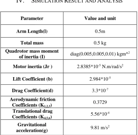
Arm Length(l) 0.5m Total mass 0.5 kg Quadrotor mass moment
of inertia (I) diag(0.005,0.005,0.01) kgm^ 2
Motor inertia (Jr ) 2.8385*10-5N.m/rad/s2 Lift Coefficient (b) 2.984*10-5 Drag Coefficient(d) 3.3*10-7 Aerodynamic friction
Coefficients (K1,2,3) 0.3729
Translational drag
Coefficients (K4,5,6) 5.56*10 -4
Gravitational
mission of the controller is to bring the quadrotor from 6meter to the ground (0meter) as soon as possible. As expected, the controller brings the quadrotor to the ground. The controller requires 140 second (2 minute & 20 second) to accomplish the mission.
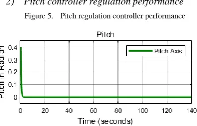
2) Pitch controller regulation performance Figure 5. Pitch regulation controller performance
In figure 5, the result shows the regulation controller performance of pitch controller. As we see from the figure, the quadrotor initially has pitch inclination angle of 10 degree or 0.174 radian with angular speed of 0.1 degree per second. The mission of the controller is to bring the quadrotor pitch inclination to zero degree. As expected, the controller brings the quadrotor pitch inclination to zero degree at a time of 2 seconds.
3) Roll controller regulation performance Figure 6. Roll regulation controller performance
In figure 6, the result shows the regulation controller performance of roll controller. As we see from the figure, the quadrotor initially has roll inclination angle of 10 degree or 0.174 radian with angular speed of 0.1 degree per second. The mission of the controller is to bring the quadrotor roll inclination to zero degree. As expected, the controller brings the quadrotor roll inclination to zero degree at a time of 3.2 seconds.
4) Yaw controller regulation performance Figure 7. Yaw (heading) regulation controller performance
In figure 7, the result shows the regulation controller performance of yaw controller. As we see from the figure, the quadrotor initially has yaw inclination angle of 10 degree or 0.174 radian with angular speed of 0.1 degree per second. The mission of the controller is to
bring the quadrotor yaw inclination to zero degree. As expected, the controller brings the quadrotor yaw inclination to zero degree at a time of 1.7 seconds.
5) Control signal for regulation
Figure 8. Altitude control signal for regulation control
In figure 8, the result shows the altitude control signal of the controller. The control signal is in practical region. The practical region is within 0 to 50 newton force interval. The motors can generate this amount of thrust force with 3000-rpm speed. With 3000-rpm speed, the motors can generate 6-newton force.
Figure 9. Pitch control signal for regulation control
In figure 9, the result shows the pitch control signal of the controller. The control signal is in practical region. The practical region is within 0 to 5 newton-meter torque. One motor can produce 1.6 newton at 3000 rpm. Making one motor stationary and other one rotates at 3000 rpm can get 0.8 newton meter torque. From the figure, the maximum bound on pitch control signal is 0.6 newton meter, which is less than 0.8 newton meter.
Figure 10. Roll control signal for regulation control
signal is 0.45 newton meter, which is less than 0.55 newton meter.
Figure 11. Yaw control signal for regulation control
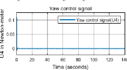
In figure 11, the result shows the yaw control signal of the controller. The control signal is in practical region. The practical region is within 0 to 3 newton-meter torque. One motor can produce 1.1 newton at 2500 rpm. Making one motor stationary and other one rotates at 2500 rpm can get 0.55 newton meter torque. From the figure, the maximum bound on yaw control signal is 0.12 newton meter, which is less than 0.55 newton meter.
ACKNOWLEDGMENT
I wish to record my deep sense of gratitude and profound thanks to my research advisor Dr. N. Suthanthira Vanitha, Associate Professor, Department of Electrical and Computer Engineering, Addis Ababa science and Technology University , Ethiopia, for her keen interest, inspiring guidance, constant encouragement with my work during all stages, to bring this paper into fruition.
CONCLUSION
In this paper, the nonlinear dynamic model of quadrotor is derived using Lagrange formalism. The model contains two parts namely translational and rotational dynamics (Euler-angle dynamics). The nonlinear model incudes the gyroscopic moments induced due to rotational motion of quadrotor body & propellers mounted on rotors. Besides, aerodynamic friction moment & force are considered in the model-ling. After the derivation of dynamic model, nonlinear control strategy (higher-order SMC) based on super-twisting algorithm is designed.
In order to verify the performance and efficiency of the controller, a simulation is done via Matlab/Simulink. The higher order SMC is designed for four output-controlled variables separately. The controlled variables are altitude, pitch, roll and yaw. The higher-order SMC implemented on the physical system for regulation problem. The controller is very effective; it can regulate the physical system with fast & smooth response and good stability. The control effort used by the controller to regulate the system is so small and within practical limit. Overall, the second-order SMC controller designed for the quadrotor system is efficient and having very good performance.
REFERENCES
[1] Vachtsevanos, Kimon P. Valavanis, George J., Handbook UAV, New York, London: Springer, 2015.
[2] R. Jategaonkar, Flight vehicle system identification a time domain methodology, Reston, Virginia: American Institute of Aeronautics and Astronautics Inc, 2015.
[3] Q. Quan, Introduction to Multicopter Design and Design, Beijing,china: Springer, 2017.
[4] D. Norris, Build Your Own Quadcopter, New York, Chicago: McGraw-Hill Education, 2014.
[5] P. Johan From, J. Tommy Gravdahl, K. Ytterstad Pettersen, Vehicle Manipulator System, Verlag, London: Springler, 2014. [6] D. Lee, H. Jin Kim, and S. Sastry, "Feedback linearization vs.
adaptive sliding mode control for a quadrotor helicopter," International Journal of Control Automation and Systems,, vol. 3, no. 7, pp. pp. 419-428, 2009.
[7] S. Bouabdallah, A. Noth, and R. Siegwart, "PID vs LQ control techniques applied to an indoor micro quadrotor," in in International Conference on Intelligent Robots and Systems, 2004.
[8] S. Bouabdallah, "Design and Control of Quadrotors with Application to Autonomous Flying," OAI, MSc thesis Zurich, vol. 10, no. 5775, 2007.
[9] A. Rezoug, M. Hamerlain, Z. Achour and M. Tadjine, "Applied of an Adaptive Higher Order Sliding Mode Controller to Quadrotor Trajectory Tracking," in IEEE International Conference on Control System, Computing and Engineering, Penang, Malaysia, November, 2015.
[10] O. Gherouat, D. Matouk, A. Hassam and F. Abdessemed, "Modeling and Sliding Mode Control of a Quadrotor Unmanned Aerial Vehicle," J. Automation and Systems Engineering, vol. 10, no. 3, pp. 150-157, 2016.
[11] Abraham Villanueva, B. Castillo-Toledo and Eduardo Bayro-Corrochano, "Multi-mode Flight Sliding Mode Control System for a Quadrotor," in 2015 International Conference on Unmanned Aircraft Systems (ICUAS), Denver, Colorado, USA, June, 2015.
[12] Yi Kui, Gu Feng, Yang Liying, He Yuqing, Han Jianda, "Sliding Mode Control for a Quadrotor Slung Load System," in Proceedings of the 36th Chinese Control Conference, Dalian, China, July 26-28, 2017.
[13] S. Bouabdallah, A. Noth and R. Siegwart, PID vs. LQ Control Techniques Applied to an Indoor Micro Quadrotor, Proceedings of the 2004 IEEE/RSJ International Conference on Intelligent Robots and Systems, pp. 2451–2456, Sendai, Japan, October 2004.
[14] S. Khatoon, D. Gupta, and L.K. Das, PID and LQR control for a Quadrotor: Modeling and simulation, Proceedings of the 2014 International Conference on Advances in Computing, Communications and Informatics, pp. 796–802, New Delhi, September 2014.
[15] V.G. Adr, A.M. Stoica and J.F. Whidborne, Sliding mode control of a4Y octorotor, UPB Scientific Bulletin, Series D: Mechanical EngineeringJournal, vol. 74, no. 4, pp. 37-52, 2012.
[16] E-H. Zheng, J-J. Xiong and J-L. Luo, Second Order Sliding ModeControl for a Quadrotor UAV, ISA Transactions, vol. 53, no. 4, pp. 1350–1356, 2014.
[17] L. Besnard, Y.B. Shtessel and B. Landrum, Quadrotor Vehicle Controlvia Sliding Mode Controller Driven by Sliding Mode Disturbance Observer, Journal of the Franklin Institute, vol. 349, pp. 658–684, 2012.
[18] J-J.E. Slotine and W. Li, Applied nonlinear control, Prentice-Hall, Englewood Cliffs, New Jersey, 1991.
[19] G.V. Raffo, M.G. Ortega and F.R. Rubio, An Integral Predictive/Nonlinear H1 Control Structure for a Quadrotor Helicopter, Automatica, vol. 46, no.1, pp. 29–39, 2010. [20] S. Islam, J. Dias and L.D. Seneviratne, Adaptive tracking
control for Quadrotor unmanned flying vehicle, Proceedings of the 2014 IEEE/ASME International Conference on Advanced Intelligent Mechatronics (AIM),pp. 441–445, Besanon, France, July 2014.
![Figure 1. Mechanical structure and configuration of quadrotor with related frames [9]](https://thumb-us.123doks.com/thumbv2/123dok_us/7804980.2084897/2.595.62.279.252.491/figure-mechanical-structure-configuration-quadrotor-related-frames.webp)