Vol 2, No 2 (2016)

(1)

JEEECCS, Volume 2, Issue 4, pages 21-28, 2016

Comparative study of three practical IMC

algorithms with inner controller of first and

second order

Vasile CÎRTOAJE

Department of Control Engineering, Computer Science and Electronics

Petroleum-Gas University Ploiesti, Romania [email protected]

Alina-Simona BĂIEȘU

Department of Control Engineering, Computer Science and Electronics

Petroleum-Gas University Ploiesti, Romania

Abstract -The structure of the studied IMC algorithms incorporates a plant model of first or second order plus deadtime (which can be obtained experimentally from the plant response to a step input) and a realizable inner controller of first or second order. The inner controller has not a tuning filter time constant as usual, but a tuning gain K that can be used by the process operator to generate a stronger or weaker control action. All algorithms have mainly four parameters: the tuning gain K and three model parameters (the model steady-state gain, the model deadtime and the model transient time). Some numerical applications are presented to show the control performance of each proposed algorithm for both proportional-type plants with and without overshoot.

Keywords: first/second order, overdamped/underdamped, overshoot, plant model, deadtime, IMC design.

I. INTRODUCTION

In the Internal Model Control (IMC) strategy, if a model of the controlled plant can be determined, then it can be used explicitly in the design of the controller, even the model is an approximate one. In the control system domain, the IMC concept was introduced and consolidated by Garcia and Morari in 1982, but similar concepts have been used previously by other researchers [2,8,9,14]. Theoretically, the complexity of a controller designed by the IMC method depends mainly on the complexity of the plant model and the control system performance stated by the designer.

The IMC design can provide a qualitatively better performance than PID design, especially for the plants with large deadtime [1,12,13]. In addition, the IMC design leads in some particular cases to a PID structure. Even if the plant model is imperfect, it is still possible to design an IMC controller without concern for the stability of the closed-loop control system, but only for the control performance. For many plant models, the classical PID controllers can be viewed as equivalent parameterizations of IMC controllers [1,15]. The traditional IMC design of the controller depends on the plant transfer function.

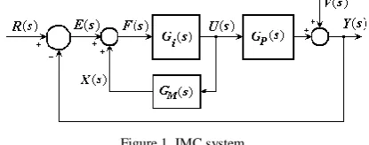
The standard IMC configuration is shown in figure 1, where G s_P( ) is the plant transfer function, G_M( )s - the model transfer function, G s_i( )- the inner controller transfer function, ( )Y s - the controlled variable, U s( )- the control (manipulated) variable, ( )R s - the reference (setpoint), E s( )- the error variable and V s( ) - the disturbance variable [2,3,4,5,6].

Figure 1.IMC system.

The transfer function between the controlled variable Y and the reference variable R has the expression

( ) ( ) ( )

1 ( ( ) ( )) ( )

P i YR

P M i

G s G s

G s

G s G s G s 

  , (1)

while the transfer function between the controlled variable Y and the disturbance variable V is

( ) 1 ( ) 1 ( ) ( )

1 ( ( ) ( )) ( )

M i

YV YR

P M i

G s G s

G s G s

G s G s G s 

  

  . (2)

Under the assumption that

(0) 1 (0) i

M

G G

 , (3)

it follows that

G_YR(0)1, G_YV(0)0.

(2)

inner controller transfer function G si( ) is the inverse of the model transfer function G_M( )s , i.e.

( ) 1 ( ) i

M G s

G s

 . (4)

If this condition is satisfied, then

G_YR( )s 1, G_YV( )s 0,

therefore ( )y t r t( ) for any time and any disturbance ( )

v t . Thus, to design an ideal control system, it is not necessary to have a perfect model, which means that

( ) ( )

M P

G s G s . Unfortunately, the inner controller cannot perfectly invert the plant dynamic model. Therefore, the classical IMC design methodology follows mainly two aims: to find a plant model as accurate as possible and a suitable proper inverse of the plant model [4,10,14,16].

The further section presents a practical approach of the IMC method starting from the hypothesis that, whatever the controlled plant (with or without overshoot), the plant model has a unique form (of first or second order plus deadtime).

Other practical features of the three control algorithms are the use of the tuning gain K instead of a tuning filter time constant (as usual) and the possible extension of the studied algorithms to control integral-type plants or even unstable plants.

II. DESCRIPTIONOFTHECONTROL ALGORITHMS

In this paper, the plant is considered with deadtime and of proportional-type (with no pole and no zero at the origin, i.e. with a steady-state gain nonzero and finite). A first-order plus deadtime plant model has the transfer function

₁ 1 ( ) 1 Ms M M M K e G s T s   

 , (5)

where K_M is the model steady-state gain, T_M₁- the model time constant and _M- the model deadtime. For the second-order plus deadtime model, we consider the transfer function with double time constant

₂ 2 2 ( ) ( 1) Ms M M M K e G s T s   

 . (6)

The time constants T_M₁ and T_M₂ can be easily obtained from the plant response ( )y t to a step plant input ( )u t using the relations

₁ 4 trP M

T

T  , (7)

₂ 6

trP M

T

T  , (8)

where T_trP is the transient time of the plant response ( )

y t (which does not include the deadtime). More precisely,

TtrP t1 , (9)

where  is the process dead time and t₁ is the settling time, when the response y attains 98 % of its steady-state value, that is

y t( )₁ 0.98 ( )y . (10) For the plant model (5), we will use the inner controller ₁ 1 1 1 ( ) ( 1) M i M T s G s

K T s  

 , (11)

while for the plant model (6), we will use either the inner controller (11) or

2 2 2 ₂ 2 ( 1) ( ) ( 1) M i M T s G s

K T s  

 , (12) where the filter time constants T₁ and T₂ were introduced to make the inner controller realizable (to have the number of poles equal to the number of zeros). The positive time constants T₁ and T₂ are lower bounded to avoid excessive noise amplification and to accommodate to the modeling error. In the traditional IMC strategy, the filter time constant is the tuning parameter of the controller, used by the process human operator to change the magnitude of the control action.

Using the substitutions

T₁ TM1 K

 , T₂ TM2 K

 , (13)

the proportional gain K (with standard value 1) is introduced as tuning parameter. The inner controllers (11) and (12) become as follows:

₁ 1 1 1 ( ) ( 1) M i M M T s G s T K s K  

 , (14)

2 2 2 2 2 ( 1) ( ) ( 1) M i M M T s G s T K s K  

 . (15)

For both controllers (14) and (15), the initial value (0 )

u _ and the final value ( )u of the response ( )u t to a unit step reference are

(0 ) i( ) M K

u G

K

    . (16)

( ) 1 P

u K

  . (17)

By increasing/decreasing the tuning gain K , the process human operator can make the control action stronger/weaker.

The magnitude coefficient M of the controllers (14) and (15), defined as the ratio between the initial value (0 )u _ and the final value ( )u of the response

( )

u t to a unit step input, is given by

(0 ) ( )

( ) (0)

i i u G M K u G     

 . (18)

In the case K1, the inner controllers (14) and (15) become identical and purely proportional:

_i₁( ) _i₁( ) 1 M

G s G s K

(3)

In this particular case, if the model is perfect, then the control system response ( )u t to a unit step reference is a step function of magnitude 1/K_P, i.e.

( ) 1 1( ) P

u t t

K

  .

Actually, because of the modeling error, the form of the response ( )u t is only close to a step form.

The control algorithms has four parameters: a tunable control gain K (with standard valueK1), which can be used by the process operator to get a strong or weak control action, and three plant parameters, that can be easily determined experimentally: the model steady-state gain K_M , the model deadtime



_M and the transient time of the model response to a step input T_trM. There is a simple procedure to verify online if the plant parameters have appropriate values and to adjust these values in order to obtain a good plant model. To make this, it only needs to set K1 and to compare the controller response to a step reference with the ideal response in step form.

The discrete equivalents of the continuous models (5) and (6) have respectively the discrete transfer functions 1 1 0 1 ₁ 1 (1 ) ( ) 1 lM M M

K p z

G z p z     

 , (20)

1 2 2 0

2 _{1 2}

2 (1 ) ( ) (1 ) lM M M

K p z

G z p z     

 , (21) where

/ ₁ 4 / 1 T TM T TtrM

p e e ,

_p₂_eT T/ M2_e6 /T TtrM_, T is the sampling time and l_M is the integer value of the ratio between the model deadtime and the sampling time; that is,

l_M M T 

 

  _ _. (22) The discrete equivalents of the continuous inner controllers (14) and (15) have respectively the discrete transfer functions 1 1 0 1 ₁ 1

1 (1 )

( )

1 i

M

K r K z

G z

K r z

    

 

 , (23)

1 2 2

0

2 _{1 2}

2

1 [ (1 ) ]

( )

(1 )

i

M

K r K z

G z

K r z

    

 

 , (24)

where

_r₁_eKT T/M1_e4KT T/trM _, _r₂_e KT T/M2_e6 KT T/trM_.

The proposed algorithms follow by combining the plant models GM1 and GM2 with the inner

controllers G_i₁ and G_i₂: G_M₁+G_i₁ - algorithm 1;

2

M

G +Gi1 - algorithm 2; GM2+Gi2 - algorithm 3.

The discrete equations of the proposed control algorithms are given by the following equations.

algorithm 1:

1 1 1 1

1

1 1 1

(1 )

1 k k k

k k M _{k lM}

k k k

k k k k

M M

e r y

p x K p u

f e x

K r K

u r u f f

K K

x

_ _ _

      _ _ _            

, (25)

algorithm 2:

2 2

2 1 2 2 2 1

1

1 1 1

2 (1 )

1 k k k

k k k M _{k lM}

k k k

k k k k

M M

e r y

p x p x K p u

f e x

K r K

u r u f f

K K

x

_ _ _ _

      _ _ _ _            

, (26)

algorithm 3:

2 2

2 1 2 2 2 1

2 2

2 1 2 2 1 2

2 (1 )

(27)

1

2 ( 2 )

k k k

k k k M _{k lM}

k k k

k k k k k k

M e r y

p x p x K p u

f e x

u r u r u Kf K Af A f

K

x

_ _ _ _

                   _ _ _ _ _  where 2 1

A  r K .

Remark 1. In order to reduce to zero the initial magnitude of the controller output u(0 )_ for a reference step, a low pass pre-filter with the transfer function

( ) 1 1 F F G s T s 

 (28)

can be used on the reference signal. Choosing a filter time constant 0 10 tr F T

T  , (29)

where T_tr0 is the transient time of the closed-loop control system with T_F0 to a step reference, provides a suitable slowness of the controller output

u.

Remark 2. The presented control algorithms can be also used to control a proportional-type plant with overshoot. The basic idea is to use a model steady-state gain larger than the plant steady-steady-state gain,

K_M (1 2 )K_P, (30)

(4)

( )

u t not excessively oscillatory. The tuning gain K can be decreased to reduce a possible too large overshoot of the plant response to a step reference.

III. SIMULATIONRESULTS

The presented control algorithms will be used to control two proportional-type plants with deadtime, one without overshoot and another with overshoot. All simulations are made using MATLAB/ SIMULINK environment.

A. Consider a proportional-type plant with deadtime and without overshoot having the transfer function

5

2( 1) ( )

(4 1)(8 1)(10 1) s P

s e

G s

s s s

  

   .

From the plant unit step response in Figure 2, it follows that

K_M 2,  _M 6, T_trM 64.

Figure 2.Plant response to a unit step input.

First algorithm. The first control algorithm provides the closed-loop control system responses to unit step reference in Figures 3, 4 and 5. Since the controller response in Figure 3 (for K1 and T_F0) is not close to a step form, it follows that the first-order model with dead time (5) cannot describe with sufficient accuracy the plant sluggishness. However, the control system responses in Figure 4 (K0.85 and T_F0) and Figure 5 ( K0.85 and T_F

0_/10 ₄

tr

T  ) have a transient time of approximately 40, which is sufficiently small for the given controlled plant.

Figure 3.Control system responses to a unit step reference for K1 and TF0.

Figure 4.Control system responses to a unit step reference for K0.85 and TF0.

Figure 5.Control system responses to a unit step reference for K0.85 and TF4.

Second algorithm. The second control algorithm provides the control system responses to unit step reference in Figures 6, 7 and 8. We can see that the controller response in Figure 6 (K1 and T_F0) is close to a step form, therefore the second-order model with deadtime (6) can describe with sufficient accuracy the plant dynamics. The control system responses in Figure 7 (K 3 and T_F0) and Figure

8 (K3 and 0_/10 _2.4

F tr

T T  ) are sufficiently fast for the given controlled plant. From these responses, we can see that the transient time is approximately 24, hence smaller than the one obtained with the first control algorithm.

(5)

Figure 8.Control system responses to a unit step reference for K3 and TF2.4.

Third algorithm. The third control algorithm yields the control system responses to unit step reference in Figure 6 (K1 and T_F0), Figure 9 (K8 and

0 F

T  ) and Figure 10 ( K8 and 0_/10

F tr T T 1.5

 ). The responses in Figures 9 and 10 are very fast for the given controlled plant. According to these responses, the transient time is approximately 15 (hence smaller than the one provided with the second control algorithm), but the magnitude coefficient M of the controller response ( )u t is too large for T_F0

(M K8). For 0_/10 _1.5

F tr

T T  , the magnitude coefficient M reduces to 4 .

Figure 10.Control system responses to a unit step reference for K8 and TF1.5.

B. Consider now a proportional plant with deadtime and overshoot having the transfer function

5 2

2(15 1) ( )

(4 1) (5 1) s P

s e

G s

s s

  

  .

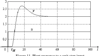
From the plant unit step response in Figure 11, it follows that K_P2,  _P 5 and  36%0.36. We will choose



M 5 and

K_M (1 2 )K_P (1 2 0.36)24.4.

Figure 11.Plant response to a unit step input.

First algorithm. Good plant responses to a unit step reference are obtained for T_tr_M 4 . The control system responses for K1 and K0.5 are shown in Figures 12 and 13. For T_tr_M 9 and K1, the plant response to a unit step reference is too sluggish (Fig. 14), while for T_tr_M 2 and K1, both the plant response and the controller response are excessively oscillatory (Fig. 15).

Figure 12.Control system responses to a unit step reference for K1, KM4.4 and TtrM4.

Figure 13.Control system responses to a unit step reference for K0.5, KM4.4 and TtrM4.

(6)

Second algorithm. Good plant responses to a unit step reference are obtained for T_tr_M 4.The control system responses for K1 and K0.5 are shown in Figures 16 and 17.

Figure 17.Control system responses to a unit step reference forK0.5, KM4.4 and TtrM4.

Third algorithm. Good plant responses to a unit step reference are obtained for T_tr_M 4 . The control system responses for K1 and K0.5 are shown in Figures 18 and 19.

Figure 19.Control system responses to a unit step reference forK0.5, KM4.4 and TtrM4.

IV. CONCLUSIONS

The structure of the studied practical IMC algorithms inserts a realizable inner controller of first or second order (C_i₁ and C_i₂) and a plant model of first or second order plus deadtime (M₁ and M₂), which can be easily obtained from the plant response to a step input. The three control algorithms are obtained by combining the inner controller type with the plant model type ( C_i₁ and M₁ for the first algorithm, C_i₁ and M₂ for the second algorithm,

2 i

C and M₂ for the third algorithm).

All control algorithms have mainly four parameters: three model parameters (the model steady-state gain K_M, the model deadtime



_M and the transient time of the model response to a step input TtrM ) and a tuning gain K with standard value 1 , which can be used by the human process operator to increase or decrease the magnitude of the control action. If K1 and the plant model has a high accuracy, then the controller response to a step reference is close to a step form. Analysing the deviation of the controller response from the ideal step form, we can adjust online the model parameters to improve the model accuracy.

Note that for all control algorithms, if no filter is on the reference signal, then the initial value (0 )u _ of the controller response ( )u t to a unit step reference is equal to the ratio K K/ _M.

(7)

better than the classical PID algorithm due to its superior control performance and the simplicity of the controller tuning procedure.

A contribution of the paper which emphasizes its practical feature consists in using the tuning gain K with standard value 1 instead of a tuning filter time constant as usual. Other main contribution is the extension of the studied algorithms to control proportional plants with overshoot.

A further research direction might be the extension of the studied algorithms to control integral-type plants and unstable plants. A method to do this is to turn the original plant into a proportional-type plant by means of a feedback path of pure proportional-type.

V. REFERENCES

[1] Adegbege, A., Heath, W., IMC Design for Input-Constrained Multivariable Process, AIChE Journal, Vol. 57, Issue 12: 3459-3472, 2011.

[2] Bengtsson, G., Output regulation and internal models - a frequency domain approach, Automatica, 13(4): 333-345, 1977.

[3] Bequette B.W., Process Control, Modeling, Design, and Simulation, Prentice Hall, 2003.

[4] Brosilow, C., Joseph, B., Techniques of Model-Based Control, Prentice Hall PTR, 2002.

[5] Chen, C.T., Linear System, Theory and Design, Third Edition, New York, Oxford University Press, 1999.

[6] Cirtoaje, V., Algoritm de tip IMC pentru reglarea proceselor supraamortizate, Buletinul Universităţii “Petrol-Gaze” din Ploieşti, Vol. LVII, Seria Tehnică, 2, 25-30, 2005.

[7] Cirtoaje, V. , Process Compensation Based Control, Buletinul Universităţii “Petrol-Gaze” din Ploieşti, Vol. LVIII, Seria Tehnică, 1, 48-53, 2006.

[8] Francis, B., Wonham, W., The internal model principle of control theory, Automatica , 12(5), pp. 457-465, 1976. [9] Garcia, C., Morari, M., Internal model control. A unifying

review and some new results, Ind. Eng. Chem. Proc. Des. Dev., vol. 21, no. 2, pp. 308-323, 1982.

[10] Horn, I., Arulandu, J., Gombas, C., VanAntwerp, J., Braatz, R., Improved Filter Design in Internal Model Control, Ind. Eng. Chem. Res.,35, 3437-3441, 1996.

[11] Marlin, T., Process Control, New York, McGraw – Hill, Inc.. 1995.

[12] Ogawa, H., Tanaka, R., Murakami, T., Ishida, Y., Designed of IMC Based on an Optimal Control for a Servo System,

Journal of Control Science and Engineering, Article ID 689767, 5 pages, 2015.

[13] Qiu, Z., Sun, J., Jankovic, M., Santillo, M., Nonlinear IMC desing for wastegate control of a turbocharged gasoline engine, Control Engineering Practice, 46: 105-111, 2016. [14] Rivera, D., Morari, M., Skogestad, S., Internal Model Control

- PID Controller Design, Ind. Eng. Chem. Process Des. Dev., 25, 252-265, 1986.

[15] Saxena, S., Hote, Y., Advances in Internal Model Control Technique: A Review and Future Prospects, IETE Technical Review, 29(6):461- 472, 2012.

(8)