DETERMINANTS OF USING RENEWABLE ENERGY
RESOURCE: PANEL DATA ANALYSIS
Cemil Serhat Akın
Associate Professor, Mustafa Kemal University,faculty of Economics and Administrative
Sciences,Hatay, Turkey
Cengiz Aytun
Associate Professor, Çukurova University,faculty of Economics
and Administrative
SciencesAdana, Turkey
İzzettin Ulusoy
Assistant Professor,Antakya Vocational College Hatay,
Turkey
ABSTRACT
Although there are many studies upon questioning the relation between the economic growth and environmental quality, there are a few studies which questioned relationship between the institutional quality, environmental quality and human development index. For this reason aim of this study is to analyze relationship between renewable energy usage and per capita income, educational expenditure, institutional quality index and human development index. The datum for countries which belong to middle income group which covers the period between the years from 2001 to 2012 was examined by the panel data analysis method. The obtained results support that there is a bilateral causality relationship between renewable energy resources and human HDI in the short run. In the long run, it was shown that income level, educational expenditure institutional quality and human development index cause of renewable energy resources.
Key words
: Renewably energy resources, Institutional Quality, Human development index, Panel Data Analysis.
1.
INTRODUCTION
While macroeconomic policies aim to increase production, they does not have the necessary precaution for environmental degradation. Policies that pay attention to environmental degradation take more carbon emissions into account. The primary reason for considering carbon emissions is global warming. Many international programs are seeking solutions to the global warming problem. Particularly after the Second World War, developments in production technologies initiated the era of mass production and the high energy needed in this process also initiated the global warming process. The rapid increase in CO2 emissions with the use of primary energy sources
has triggered global warming. Thus, the increase in global warming is at the top of the list of problems to be solved by threatening human life.
Since the institutional arrangements of developed countries are complete and the undeveloped countries do not have sufficient factor equipment for production, the creation of environmental pollution is more likely to occur in developing countries. For this reason, global warming prevention programs are mostly directed towards developing countries. In particular, incentives of governments to use renewable energy sources form the basis of these programs. The aim of this study is to analyze the determinants of renewable energy use econometrically. For this reason, unlike other studies, including the use of renewable energy, per capita national income, education expenditures, and analysis, the institutional quality and human development index has also been included in the study. In the analysis, countries in the middle income group were used because they were seen as developing responsible for environmental degradation. The data of the 13 countries in the middle income group, which can be accessed within the scope of the study, were analyzed by panel data analysis method for the period from 2001 to 2012. In the next part of the study, the previous studies on the subject will be presented, and in the third part information about the data included in the study and the method used will be given. In the fourth chapter the findings obtained will be presented and the study will be finalized with results and policy recommendations.
2.
RELATED LITERATURE
In the studies in which the relationship between the environmental degradation and economic growth is examined, CO2 emission and
per capita income variants are more likely to be used and the relationship is explained in the context of the Environmental Kuznets Curve (EKC)) hypothesis. S. Kuznets (1955) emphasizes that in the countries in the development process income inequality with development will initially increase but then trend in income inequality will decrease and stop as economic development continues.
In the development process with per-capita income, the curve “U” showing at first an increasing and then declining tendency between growth and income inequality appeared in the literature as "Kuznets Curve" (Panayotou (1993). Later, Kuznets' this study was adapted for environmental degradation and the Environmental Kuznets Curve (EKC) was obtained when the income distribution axis in the standard Kuznets Curve was replaced by environmental deterioration.
First, Grossman and Krueger concluded that the relationship between income level and environmental quality has been related to the fact that income growth increases environmental damage to a certain level and decreases environmental degradation after the threshold level (Grossman and Kruger, 1991). In his work on the relationship between institutional quality and environmental degradation, Panayatou has argued that economic growth will prevent environmental degradation and that this will be achieved through effective actuation of institutions. (Panayotou 1997) Panayotou has used institutional quality indicators created by Knack and Keefer in a panel data analysis that he has done for 30 countries. With the emergence of the new institutional economics literature, the relationship between institutions and many variables has begun to be questioned. One of the relations that are questioned is the environmental interaction with the institutions. In this process, the effective process of institutions creates institutional quality and reduces environmental degradation (Leitaou, 2010; Culas, 2007; Bhattari and Hamming, 2001; Knack and Keefer, 1995; Panayotou, 1997). The development of institutional quality slows down environmental degradation by reducing opportunism and corruption (Gagliardi, 2008: 3).In economies with opportunistic rant seeking,while transaction costs are increasing, resources are shifting from productive areas to nonproductive areas (Knack and Keefer, 1997).The understanding of production, which is prevalent in economies where corruption and bribery are occurring, is based on the consumption of resources in a short period of time rather than the effective consumption of resources.
It is thought that there is a negative relation between environmental deterioration and education level. This interaction can take place through two mechanisms. First, level of higher education facilitates the formation of social consciousness and facilitates the solution of common problems together. Higher education level increase the power and efficiency of civil society organizations and create pressure on the implementation of environmental standards (Bimonte, 2002; Dasgupta, Laplante, Wang, & Wheeler, 2002; Wheeler, 2001). Secondly, the higher level of education provides the creation of environmentally sensitive technologies, in particular the human capital necessary for the use of renewable energy. In Aytun (2014) study, he stated that the increase in the level of higher education has the effect on reducing carbon dioxide emissions by allowing the use of renewable energy.
3.
DATA AND MODEL
study World Governance Indicator which was created by the World Bank, was used as a corporate quality indicator. Other variants included in the study such as the use of renewable energy sources, per capita income, education expenditures and data used for the human development index are derived from the World Bank Database. In the formation of the institutional quality index, data on the level of corruption in the country, the effectiveness of the government, political stability, the quality of the regulations, the rule of law, freedom of thought and accountability level were used and the geometric means of these data were taken.
The methodology of Amartya Sen (1999) was followed in the formation of human development index. The explanations and sources of data for the period between 2001 and 2012 are presented in Table 1.
Table 1: Variables used in the study
KOD DESCRIPTION SOURCE
LREN Renewable energy usage (Metric tons per capita) WDIa
LGDP National income per capita (With 2005 prices US$) EFWb
LEDUX Education expenditure per capita- (With 2005 prices) WDIa
LIQ Institutional Quality Index WDIa
LHDI Human development index WDIa
a
The World Bank World Development Indicators: http://databank.worldbank.org
b
Economic Freedom of The World 2014 Annual Report: http://www.cato.org/economic-freedom-world
In this study, panel data analyses were used to estimate the determinants of the use of renewable energy sources. Panel data analysis is seen as a stronger analysis than the time series analysis because it monitors both the time-specific effect and the country-specific effects. The determinants of renewable energy sources are estimated within the model set out below.
While in Equation 1 “i” expresses the countries included in analysis and “t” expresses the time period, the expression "L" in front of the variables indicates that all variables are subject to analysis in logarithmic form.
LRENi,t= αi+ β1LGDPi,t + β2LEDUXi,t+β3LIQi,t + β3HDIi,t +εit, (1)
A positive relationship is expected between education expenditure and institutional quality and the use of renewable energy sources in the equation created. The direction of the relationship between per capita income and the use of renewable energy may vary. Especially in the underdeveloped countries, the energy needed for fast growth targets is being tried to be met by the primary sources and the investments for the use of renewable energy required high cost can be neglected.
4.
METHOD
The use of the estimation and error correction (ECM) model of the long-run relationships among the variables within the context of the analysis is carried out in four stages (Pao and Tsai, 2011). The first stage is the unit root test. In order to perform the cointegration tests between the variables, the series must be stationary at the same level. For this purpose, four unit root tests were applied in the analysis. These tests are Phillips Perron and Levin Lin Chu unit root tests of Im, Pesaran Shin (2003), Fisher-type Augmented Dickey-Fuller (F-ADF) (Maddala and Wu, 1999: Choi, 2001).
In the second stage, cointegration tests will be applied if the series are stationary at the same level. Cointegration analyzes are used to question the existence of long-term equilibrium relations between the series. Engle and Granger (1987) stated that linear combinations of nonstationary series may be stable in long-term in their work. The most preferred method in the literature for the cointegration analysis of the series of panel data analyzes is the method developed by Pedroni (1999, 2004).
4.1. Panel Cointegration Test
Pedroni panel cointegration test is a two-stage test based on Engle-Granger (1987). In Pedroni (1999) cointegration analysis, it is tested whether there is a long term cointegration relation between variables by looking at the stability of εit residue in equation (1). In the
second stage the error terms obtained are again estimated by OLS in Eq. (2).
The tests that Pedroni has some advantages. These tests allow multiple explanatory variables to be included in the analysis. In addition, the tests also allow the predicted cointegration vector vary along the different parts of the panel and the faults to be heterogeneity along the cross-sectional units. Pedroni has developed a test statistic with a total of seven and the Ho hypothesis cointegration "no
co-integration". These tests are divided into two separate groups. The first category includes four tests pooled in the “within” dimension, and the second category contains three other tests in the "between" dimension (Asteriou and Hall, 2007). The first three of the four tests in the within test group are non-parametric tests. The first of these tests is a statistic of variance ratio type. The second is similar to the statistical Phillips-Peron (PP) (rho) statistic, and the third statistic is similar to the PP (t) statistic. The last statistic in the Within group is a parametric statistic similar to the Augmented Dickey Fuller (ADF) (t) statistic. The three statistics in the Between group use the averages of the estimated individual coefficients of each country. The first of the three tests in the second category is similar to the PP (rho) statistic, while the other two are similar to the PP (t) and ADF (t) statistics (Güvenek and Alptekin, 2010; Nazlıoglu, 2012).
4.2. Panel Coalescence Estimation (FMOLS)
The third stage to be followed after cointegration is the prediction phase of the Panel Cointegration model. Fully Modified OLS (FMOLS) is widely used in estimating cointegrated heterogeneous series in panel data analysis (Pedroni, 2000). Panel FMOLS estimator for each time series is 𝛽 𝐺𝐹𝑀∗ = 𝑁−1 𝑁𝑖=1𝛽𝐹𝑀𝑖∗ obtained by using 𝛽𝐹𝑀𝑖∗ the results obtained from Equation 1.
4.3. Granger Causality Test
While the sign of the coefficients obtained after the cointegration tests gives information about the direction of the relationship between the series, it does not give information about the direction of the causality relation. Causality analysis is needed to determine the direction of causality between the series (Nazlioglu and Soytas, 2012). For this reason, the analysis of causality was made in the fourth stage. The existence of the cointegration relationship between variables also points to the presence of at least one directional Granger causality (Engle RF, Granger CWJ.1987; Oxley L, Greasley D., 2008). Engle and Granger in their study in 1987 stated that in the causality tests while there is a cointegration relation between two nonstationary variables the VAR process performed by taking the differences of the series can produce incorrect results. For this reason, it is suggested to use vector error correction model (VECM) estimated with the adapted VAR model which is made dynamic by delayed error correction term(Narayan and Smyth, 2009; Aytun, 2014). The obtaining process of panel-based VECM is expressed in Equation 3 below. (Pao and Tsai, 2011; Belloumi, 2009). Equation 3 shows the number of countries from i = 1 to N, and the time interval t = 1 to T.Abdalla and Murinde (1997) and Pao and Tsai (2011) were followed to maximize the R2 and AIC criterion for the appropriate number of delays for each equation in equation 3.
𝛥𝐿𝑅𝐸𝑁𝑖𝑡 𝛥𝐿𝐺𝐷𝑃𝑖𝑡 𝛥𝐿𝐸𝐷𝑈𝑋𝑖𝑡
𝛥𝐿𝐼𝑄𝑖𝑡 𝛥𝐿𝐻𝐷𝐼𝑖𝑡2
= 𝛼1 𝛼2 𝛼3 𝛼4 𝛼5
+
𝛽11𝑝 𝛽12𝑝 𝛽13𝑝 𝛽14𝑝 𝛽15𝑝 𝛽21𝑝 𝛽22𝑝 𝛽23𝑝 𝛽24𝑝 𝛽25𝑝 𝛽31𝑝 𝛽32𝑝 𝛽33𝑝 𝛽34𝑝 𝛽35𝑝 𝛽41𝑝 𝛽42𝑝 𝛽43𝑝 𝛽44𝑝 𝛽45𝑝 𝛽51𝑝 𝛽52𝑝 𝛽53𝑝 𝛽54𝑝 𝛽55𝑝 𝑟
𝑝=1
𝛥𝐿𝑅𝐸𝑁𝑖𝑡−𝑝 𝛥𝐿𝐺𝐷𝑃𝑖𝑡−𝑝 𝛥𝐿𝐸𝐷𝑈𝑋𝑖𝑡−𝑝
𝛥𝐿𝐼𝑄𝑖𝑡−𝑝 𝛥𝐿𝐻𝐷𝐼𝑖𝑡−𝑝2
+ 𝜃1 𝜃2 𝜃3 𝜃4 𝜃5
𝐸𝐶𝑇𝑖𝑡−1+ 𝜀1𝑖𝑡 𝜀2𝑖𝑡 𝜀3𝑖𝑡 𝜀4𝑖𝑡 𝜀5𝑖𝑡
(3)
5.
FINDINGS
5.1. Panel Unit Root Test Results
Table 2: Panel Unit Root Test Results
LLC PP IPS F-ADF
Variables Level First Diff. Level First Diff. Level First Diff. Level First Diff.
ΔLREN -1.468 -7.24*** 34.71 141.9*** -0.439 -6.83*** 31.64 88.77***
ΔLGDP -1.721 -4.60*** 53.64 69.36*** 1.517 -2.04*** 14.85 35.84***
ΔLEDUX -3.543 -5.13*** 26.18 47.02*** 0.932 -2.66*** 18.52 43.56***
ΔLINSQ -4.758 -2.67*** 26.13 101.1*** -0.382 -2.65*** 34.83 43.82***
ΔLHDI -0.821 -5.60*** 16.30 89.99*** 2.661 -3.41*** 8.918 50.92***
*** Expresses Statistical significance at the level of 1%. All variables are evaluated as fixed and trendy.
The number of delays is automatically determined according to the Schwarz information criterion (SIC).
5.2. Panel Cointegration Test Results
Findings from unit root test results applied to balanced panel data allow the cointegration test. The long term equilibrium relations of the series at the same level and first degree were questioned by the Pedronicointegration test. According to Pedronicointegration test results,H0hypothesis, in which there is no cointegration in four of the seven test statistics, was rejected and resulted in cointegration. In
this case, it can be said that there is a relation between variables in long term. Pedronicointegration test results are presented in Table 3.
Table 3.Pedronicointegration test results
Fixed Fixed and trendy
Within-dimension Within-dimension
Tests Test Statistics Prob. Test Statistics Prob.
Panel v-Statistic -2,652 0,996 -4.151873 1.0000
Panel rho-Statistic 2,968 0.998 4.078259 1.0000
Panel PP-Statistic -7.28*** 0.000 -10.66508 0.0000
Panel ADF-Statistic -5.02*** 0.000 -4.107223 0.0000
Between-dimension Between-dimension
Tests Test Statistics Prob. Test Statistics Prob.
Group rho-Statistic 4,292 1.000 4.750691 1.0000
Group PP-Statistic -9.32*** 0.000 -14.04127 0.0000
Group ADF-Statistic -4.10*** 0.000 -3.231691 0.0006
Notes: The 1%, 5%, and 10% critical values are respectively 1.28, 1.645, and 2.33 for the panel-v statistics and 1.28, -1.645, and -2.33 for the other statistics. The maximum delay was identified as 1 with SIC.
5.3. Panel FMOLS Estimation Results
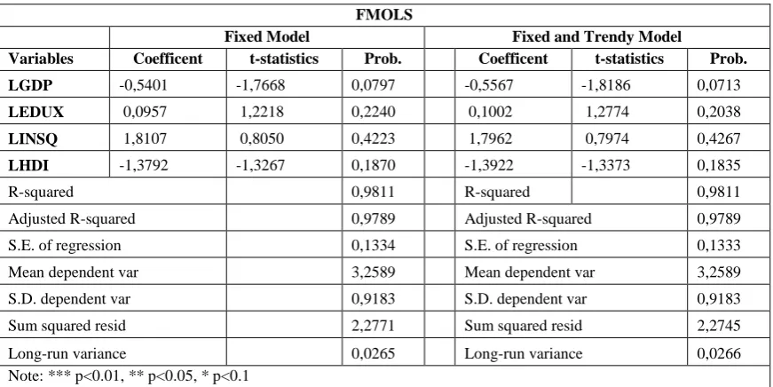
It has come to the forefront of the estimation process of cointegrated series after the series have been revealed to be in the cointegration. According to FMOLS estimation results presented in Table 4, it is seen that there is a positive relation between inflation, renewable energy use, education expenditures and institutional quality. There is no statistically significant relationship between the human development index and the use of renewable energy. According to the findings, the use of renewable energy and per capita income has been falling. This situation can be explained by the Kuznets curve. The increase in income level increases the environmental degradation in the early period and after a certain level, the environmental degradation decreases. This situation is explained by scale effect. The increase in production increases the need for energy and as a result, the consumption of cheap fossil fuels is increasing. Due to the lack of physical capital accumulation of countries with low and middle income levels, the capital required for the use of renewable energy can not be provided in these countries and fossil fuel is preferred as energy source in production. The fact that the institutional structure in the country is not developed sufficiently can not prevent the production methods and energy usage which are harmful to the environment.
technologies to them. Less-developed countries are producing with technologies that generate pollution and work with more primary energy sources until income levels reach a certain level. A statistically significant coefficient estimate between education expenditure, institutional quality, human development index and renewable energy use could not be estimated.
Table 4. Panel FMOLS Estimate Results
FMOLS
Fixed Model Fixed and Trendy Model
Variables Coefficent t-statistics Prob. Coefficent t-statistics Prob.
LGDP -0,5401 -1,7668 0,0797 -0,5567 -1,8186 0,0713
LEDUX 0,0957 1,2218 0,2240 0,1002 1,2774 0,2038
LINSQ 1,8107 0,8050 0,4223 1,7962 0,7974 0,4267
LHDI -1,3792 -1,3267 0,1870 -1,3922 -1,3373 0,1835
R-squared 0,9811 R-squared 0,9811
Adjusted R-squared 0,9789 Adjusted R-squared 0,9789
S.E. of regression 0,1334 S.E. of regression 0,1333
Mean dependent var 3,2589 Mean dependent var 3,2589
S.D. dependent var 0,9183 S.D. dependent var 0,9183
Sum squared resid 2,2771 Sum squared resid 2,2745
Long-run variance 0,0265 Long-run variance 0,0266 Note: *** p<0.01, ** p<0.05, * p<0.1
5.4. Panel VECM Causality Analysis Results
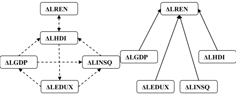
When short-run and long-run causality between variables are examined, it is seen that there is a two-way causality relationship between the human development index and the use of renewable energy. (Table 5) While the use of renewable energy increases the level of human development of the country, the increased level of development and prosperity also increases the demand for renewable energy use. The increase in income indirectly affects the use of renewable energy. Increased income affects institutional quality and human development, which indirectly affects the use of renewable energy. Similarly educational expenditures also affect the level of institutional quality and income in the country. In addition, Figure 1 and Figure 2 summarize short and long cyclical causality relationships.
Table 5.Panel VECM Causality Results
Short-term causality
[Chi-sq] Long-term causality
Series ΔLREN ΔLGDP ΔLEDUX ΔLINSQ ΔLHDI ECT ( )
ΔLREN - 3.737 0.203 1.370 11.89** -1.13***
ΔLGDP 2.361 - 9.39** 2.399 6.993 0.127*
ΔLEDUX 0.725 6.189 - 6.158 9.482* 0.381
ΔLINSQ 3.549 8.66* 8.93* - 1.545 0.008
ΔLHDI 9.18** 8.242* 0.830 12.28** - 0.025
Notes: H0: There is no causality relationship among the series. Δ: indicates that the first difference of the series is taken. ***p<0.01, ** p<0.05, * p<0.1
Figure 1.Short-term Causality Relations Figure 2. Long-term Causality Relations
6.
CONCLUSIONS
At the center of macroeconomic policies, the goal of production increase is taking place, which causes the development phenomenon to be neglected. Development has begun to be measured together with qualitative factors in the early 1990s. Especially environmental quality has become one of the important elements of development. While the energy demand in the production process appears to be the primary cause of environmental degradation, increasing the use of renewable energy to reduce this degradation has become the main policy applied by governments. In this study, to identify determinants of the use of renewable energy sources, the use of renewable energy, per capita national income, education expenditure were included in the analysis and apart from the other studies, institutional quality and human development indexes were included in the analysis. According to panel FMOLS results, there is no statistically significant coefficient for the interaction between education expenditure and change in institutional quality, human development index and renewable energy use.On the other hand, it is expected that the 1% increase in per capita income will reduce the use of renewable energy by 0.54% in the with constant model and 0.55% in the with constant and trend model. This situation also overlaps with the Pollution Heaven Hypothesis.
Investments made in countries with low institutional quality increase production while energy demand increases. In order to be able to meet the renewable energy resources needed, these resources need to be created with investments. These resources require high capital investment, and undeveloped countries that do not have such capital tend to primary energy resources, which are important in environmental degradation. In this case, environmental quality is regarded as luxury goods, corporate regulations are made with increasing income and environmental degradation is reduced. Within the context of the analysis, only the human development index and the use of renewable energy in the short term are related within the human context, while the other three variants are the reasons of the use of renewable energy source in long term. In this case, it is understood that environmental degradation can be avoided by making institutional arrangements in particular. The active role of the government in this process will improve environmental degradation more quickly.
REFERENCES
[1] Asterıou, D.,and Hall, S. G., 2007. “Applied Econometrics : A Modern Approach Using EviewsAndMicrofit”. New York: Palgrave Macmillan.
[2] Aytun C., 2014. " The Relationship Between Carbon Emission, Economic Growth and Education in Developing Economies: Panel Data Analysis", The Journal of Academic Social Sciences Studies, 27, 349-362.
[3] Abdalla, I. andMurinde, V. 1997 “Exchange Rates And Stock Price Interactions İn Emerging Financial Markets: Evidence On India, Korea, Pakistan And The Philippines”, Applied Financial Economics, 7:25-35.
[4] Bhattaraı, M., and Hammıng, M. 2001. “Institutions And The Environment Kuznets Curve For Deforestation: Across Country Analysis For Latin America, Africa And Asia”. World Development 2001;29(6),995–1010.
[5] Bimonte, S., 2002. Information Access, İncome Distribution, And The Environmental Kuznets Curve. Ecological Economics, 41(1), 145–156.
[6] Choi I.,2001. Unit Root Tests For Panel Data. Journal Of International Money And Finance, 20, 249-72.
ΔLREN
ΔLEDUX
ΔLHDI
ΔLGDP
ΔLINSQ
ΔLREN
ΔLEDUX
ΔLHDI
[7] Culas, R.J. 2007. “Deforestation And The Environmental Kuznets Curve :An İnstitutional Perspective”. Ecological Economics, 61(2–3), 429–37.
[8] Dasgupta, S., Laplante, B., Wang, H.,ve Wheeler, D. 2002. Confronting The Environmental Kuznets Curve. The Journal Of Economic Perspectives, 16(1), 147–168.
[9] Engle Rf, Granger Cwj.1987 “Co-İntegration And Error Correction: Representation, Estimation, And Testing”. Econometrica 55:251-76.
[10]Gaglıardı, F. 2008 “Institutions And Economic Change: A Critical Survey Of The New Institutional Approaches And Empirical Evidence” The Journal Of Socio-Economics, (37), 416-443
[11]Grossman, G.,M. and Krueger, A.B., 1991. Environmental İmpacts Of The North American Free Trade Agreement. Neer Working Paper No: 3914 November 1991
[12]Güvenek, Burcu andAlptekinVolkan 2010. “EnerjiTüketimiVeBüyümeİlişkisi: OecdÜlkelerineİlişkinBir Panel VeriAnalizi”, Enerji, PiyasaVeDüzenleme, Cilt:1, Sayı:2, 172-193.
[13]InternatıonalEnergy Agency, 2013. Co2 Emissions From Fuel Combustion Highlights (2013 Edition)
[14]Im Ks, Pesaranand Mh, Shin Y. 2003. “Testing For Unit Roots in Heterogeneous Panels”.Journal Of Econometrics, 115:53-74.
[15]Knack, S.,and Keefer, P. 1995. “Institutions And Economic Performance: Cross-Country Tests Using Alternative Institutional Measures”, Economics And Politics, 7, 207-227.
[16]Knack, S., and Keefer, P. 1997. “Does Social Capital Have An Economic Payoff? A Cross-Country Investigation”.Quarterly Journal Of Economics 112(4, November), 1251–1288.
[17]Kuznets, S., 1955.Economic growth and income inequality. American Economic Review, 49: 1-28.
[18]Leıtao, A., 2010. “Corruption And The Environmental Kuznets Curve: Empirical Evidence For Sulphur”. Ecological Economics, 69(11), 2191–201.
[19]Levın, Andrew; Chien- FuLın ve Chia-Shang James Chu; 2002. Unit Root Tests İn Panel Data: Asymptotic And Finite-Sample Properties. Journal Of Econometrics, 108(1), Pp. 1-24.
[20]MaddalaGs, and Wu S. 1999. “A Comparative Study Of Unit Root Tests With Panel Data And A New Simple Test”. Oxford Bulletin Of Economics And Statistics, 61: 631-52.
[21]Narayan, P.K. and Smyth, R. 2009. Multivariate Granger Causality Between Electricity Consumption, Exports And Gdp: Evidence From A Panel Of Middle Eastern Countries. Energy Policy, 37: 229-236
[22]Nazlioglu, S., 2012.“Exchange Rate Volatility And Turkish Industry-Level Export: Panel Cointegration Analysis”. The Journal Of International Trade & Economic Development :120,
[23]Nazlioglu,Saban andSoytas, Ugur, 2012. “Oil Price, Agricultural Commodity Prices, And The Dollar: A Panel Cointegration And Causality Analysis”. Journal Of Energy Economics, 34, 1098-1104.
[24]Oxley, L. and Greasley, D., (,2008), “Vector Autoregression, Cointegration and Causality: Testing for Causes of the British Industrial Revolution”. Applied Economics, 30, 1387-1397.
[25]Panayotou, T., 1993, “Empirical Tests And Policy Analysis Of Environmental Degradation At Different Stages Of Economic Development”, In Technology, Environment, And Employment, Geneva: International Labour Office.
[26]Panayotou, T. 1997. “Demystifying The Environmental Kuznets Curve: Turning A Black Box İnto A Policy Tool”. Enviroment And Development Economics;2(4),465-84.
[27]Pedroni, 1999. “Critical Values For Cointegration Tests İn Heterogeneous Panels With Multiple Regressors”, Oxford Bulletin
Of Economics And Statistics, 61(S1), 653–670.
[28]Pedroni, 2000. “Fully Modified Ols For Heterogeneous Cointegrated Panels”, B. H. Baltagi (Ed.), Advances in Econometrics
(Vol. 15, S. 93–130). Bingley: Emerald.
[29]Pedroni, 2004. “Panel Cointegration: Asymptotic And Finite Sample Properties Of Pooled Time Series Tests With An
Application to the PPP Hypothesis”, Econometric Theory, 20(03), 597–625.
[30]Pao, H., and Tsai, C. 2011. Multivariate Granger Causality Between Co2 Emissions, Energy Consumption, Fdı (Foreign Direct İnvestment) And Gdp (Gross Domestic Product): Evidence From A Panel Of Bric Countries. Energy, 36: 685 – 693.
[31]Sen, Amartya, 1999, “The ends and means of development” Chapter 2 from “Development as Freedom”, Oxford University
Press.
[32]Soytas, U., Sarı, R. 2009. “Energy Consumption, Economic Growth, And Carbon Emissions: Challenges Faced By An Un Candidate Member”. Ecol Econ; 68, 1667-75.