Graph Computation Models
Selected Revised Papers from the
Third International Workshop on
Graph Computation Models (GCM 2010)
Minimizing Finite Automata with Graph Programs
Detlef Plump, Robin Suri, and Ambuj Singh15 pages
Guest Editors: Rachid Echahed, Annegret Habel, Mohamed Mosbah Managing Editors: Tiziana Margaria, Julia Padberg, Gabriele Taentzer
Minimizing Finite Automata with Graph Programs
∗Detlef Plump1, Robin Suri2, and Ambuj Singh3
1The University of York, UK2Indian Institute of Technology Roorkee, India3Indian Institute
of Technology Kanpur, India
Abstract: GP (for Graph Programs) is a rule-based, nondeterministic program-ming language for solving graph problems at a high level of abstraction, freeing programmers from dealing with low-level data structures. In this case study, we present a graph program which minimizes finite automata. The program represents an automaton by its transition diagram, computes the state equivalence relation, and merges equivalent states such that the resulting automaton is minimal and equivalent to the input automaton. We illustrate how the program works by a running exam-ple and argue that it correctly imexam-plements the minimization algorithm of Hopcroft, Motwani and Ullman. We also prove a quadratic upper bound for the number of rule schema applications used by the program.
Keywords: Graph programs, automata minimization, rule-based programming, cor-rectness proofs
1
Introduction
GP is an experimental nondeterministic programming language for high-level problem solving in the domain of graphs. The language is based on conditional rule schemata for graph trans-formation, freeing programmers from implementing and handling low-level data structures for graphs. The prototype implementation of GP compiles graph programs into bytecode for an ab-stract machine, and comes with a graphical editor for programs and graphs. We refer to [Plu09] for an overview of the language and to [MP08] for a description of the current implementation.
In this paper, we present a case study about solving a problem with GP that as first sight may not appear to be a graph problem: the minimization of finite automata. It is natural though to represent finite automata by their transition diagrams and to view the minimization process as a sequence of transformation steps on these diagrams. Programmers can visually construct corresponding rule schemata and control the application of these schemata by GP’s commands.
We implement the minimization algorithm of Hopcroft, Motwani and Ullman [HMU07] (see also [Sha09]). This algorithm first computes the indistinguishability relation among states, called state equivalence, and then merges equivalent states to obtain a minimal automaton that is equiv-alent to the input automaton. Two states are equivequiv-alent if processing strings from either state will have the same result with respect to acceptance. While state equivalence is usually com-puted by a table-filling algorithm, in our case we directly connect equivalent states with special edges. Once the equivalent states have been determined, we merge them by redirecting edges and removing isolated nodes.
∗Work of the second and third author was done while visiting the University of York. Funding by the Department of
In Section5, we argue that our implementation is correct in that the graph program will trans-form every input automaton into an equivalent and minimal output automaton. This involves showing that the program terminates, that it correctly computes the state equivalence relation, and that the merging phase produces an automaton in which each equivalence class of states is represented by a unique state. We also show, in Section 6, that the maximal number of rule schema applications used by our program is quadratic in the size of the input automaton.
This paper is a revised and extended version of [PSS10].
2
Graph Programs
We briefly review GP’s conditional rule schemata and control constructs. Technical details (in-cluding the abstract syntax and operational semantics of GP) can be found in [Plu09], as well as a number of example programs.
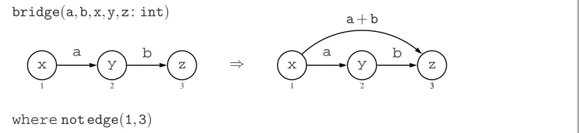
Conditional rule schemata are the “building blocks” of graph programs: a program is essen-tially a list of declarations of conditional rule schemata together with a command sequence for controlling the application of the schemata. Rule schemata generalise graph transformation rules in the double-pushout approach with relabelling [HP02], in that labels can contain expressions over parameters of type integer or string. Figure1 shows a conditional rule schema consisting of the identifier bridgefollowed by the declaration of formal parameters, the left and right graphs of the schema, the node identifiers1,2,3specifying which nodes are preserved, and the keywordwherefollowed by the conditionnot edge(1,3).
bridge(a,b,x,y,z:int)
x
1
y
2
z
3
a b
⇒ x
1
y
2 3
z
3
a+b
a b
wherenot edge(1,3)
Figure 1: A conditional rule schema
In the GP programming system [MP08], rule schemata are constructed with a graphical editor. Labels in the left graph comprise only variables and constants because their values at execution time are determined by graph matching. The condition of a rule schema is a Boolean expression built from arithmetic expressions and the special predicateedge, where all variables occurring in the condition must also occur in the left graph. The predicateedgedemands the (non-)existence of an edge between two nodes in the graph to which the rule schema is applied. For example, the expressionnot edge(1,3)in the condition of Figure1forbids an edge from node 1 to node 3 when the left graph is matched.
the preserved nodes (which are unlabelled) andΓα,gis a predicate on graph morphisms g : Lα→ G (see [Plu09]).
GP’s commands for controlling rule-schema applications include the non-deterministic one-step application of a rule schema, the non-deterministic one-one-step application of a set{r1, . . . ,rn}
of rule schemata, the sequential composition P; Q of programs P and Q, the as-long-as-possible iteration P! of a program P, and the branching statementifCthenPelseQ for programs C, P and Q. The first four of these commands have the expected effects. The branching command first checks if executing C on the current graph G can produce a graph; if this is the case, then P is executed on G, otherwise Q is executed on G.
1 2
3
4
1 2
3
→
bridge! 1
2
3
4
1 2
3
3 6
5
Figure 2: An execution of the programbridge!
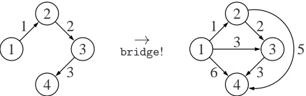
For example, Figure 2shows an execution of the program bridge!. This program makes an input graph transitive in that for every directed path of the input, the output graph contains an edge from the first node to the last node of the path. Note that the edge with label 6 can be produced by applying bridgein two different ways, performing either the addition 3+3 or 1+5. In general, a program may produce many different output graphs for the same input. The semantics of GP assigns to every input graph the set of all possible output graphs (see [Plu09,PS10]).
3
Automata Minimization
Our starting point is the abstract minimization algorithm of Hopcroft, Motwani and Ullman [HMU07] (see also [Sha09]). To fix notation, we consider a deterministic finite automaton (DFA) as a system A= (Q,Σ,δ,q0,F)where Q is the finite set of states,Σis the input alphabet,δ: Q× Σ→Q is the transition function, q0 is the initial state, and F is the set of final (or accepting) states. The extension ofδ to strings is denoted byδ∗: Q×Σ∗→Q.
Definition 1 States p and q of an automaton are equivalent if for all strings w∈Σ∗,δ∗(p,w)∈ F if and only ifδ∗(q,w)∈F.
Note that this indeed defines an equivalence relation. We say that states p and q are distin-guishable if they are not equivalent, that is, there must be some string w∈Σ∗ such that either δ∗(p,w)∈F andδ∗(q,w)∈/F, or vice-versa.
Algorithm 1 ([HMU07])
Marking phase
Stage 1:
for each p∈F and q∈Q−F do mark the pair{p,q}
Stage 2: repeat
for each non-marked pair{p,q}do for each a∈Σdo
if{δ(p,a),δ(q,a)}is marked then mark{p,q} until no new pair is marked
{For each state p, the equivalence class of p consists of all states q for which the pair{p,q} is not marked.}
Merging phase
Construct ˆA= (Qˆ,Σ,δˆ,qˆ0,Fˆ)as follows:
– Q consists of the state equivalence classes.ˆ – qˆ0is the equivalence class containing q0.
– For each X∈Q and aˆ ∈Σ, pick any p∈X and set ˆδ(X,a) =Y , where Y is the equivalence class containingδ(p,a).
– F consists of the equivalence classes containing states from F.ˆ
By the following lemma, the marking phase of Algorithm1correctly computes the state equiv-alence.
Lemma 1 ([HMU07,Sha09]) A pair of states is not marked by the marking phase of Algorithm
1if and only if the states are equivalent.
Using Lemma1, the correctness of Algorithm1can be established.
Theorem 1 ([HMU07]) The automaton ˆA produced by Algorithm1accepts the same language as A and is minimal.
In the next section, we present an implementation of Algorithm1 in GP. The correctness of the implementation is proved in Section5.
4
Implementation in GP
1. The states have labels of the form x i, where x is some integer and i∈ {0,1}. The compo-nent i is called a tag1, we require that final states have tag 1 and that non-final states have tag 0. The integer x is arbitrary, except that the initial state, and only this state, has a label of the form 1 i.
2. The transitions are labelled with strings which represent the symbols inΣ.
3. To keep the presentation simple, we assume that all states are reachable from the initial state. (It is straightforward to write a graph program that removes all unreachable states.)
The graph program implementing Algorithm 1 is shown in Figure 3, wheremark,merge
andclean upare macros. The rule schemata contained in the macros are discussed below.
main = mark; merge; clean up
mark = distinguish!; propagate!; equate!
merge = init; add tag!; (choose; add tag!)!; disconnect!; redirect! clean up = remove edge!; remove node!; untag!
Figure 3: GP program for automata minimization
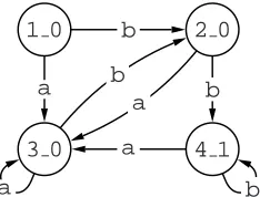
We will explain each stage of the program in Figure3, using as running example the mini-mization of the automaton in Figure4. This automaton accepts all strings over{a,b}that end in twob’s.
1 0
3 0 4 1
2 0 b
a b
a b
a
a b
Figure 4: Sample automaton with alphabet{a,b}
4.1 Marking Phase
We first need to determine which states are equivalent. For this, we implement the marking phase of Algorithm1in the macromark. The macro’s rule schemata are shown in Figure5.
The subprogram distinguish! implements Stage 1 of Algorithm 1. Given two states such that one is a final state and the other is not, by assumption, the states carry tags1and 0
respectively. In this case we mark the states as distinguishable by connecting them with two1 -labelled edges of opposite direction (drawn as a single edge with two arrowheads). The condition not edge(1,2,1)indistinguishforbids a1-labelled edge between nodes1and2to make sure thatdistinguish!terminates. The ternaryedgepredicate refines the binary predicate
1In general, a label in GP has the form x
distinguish(x,y,i,j:int)
x i
1
y j
2
⇒ x i
1
y j
2
1
wherei6=j and not edge(1,2,1)
propagate(x,y,u,v,i,j,m,n:int;s:str)
x i
1
u m
3
y j
2
v n
4
s
s
1 ⇒
x i
1
u m
3
y j
2
v n
4
s
s 1 1
wherenot edge(1,2,1)
all matches
equate(x,y,i,j:int)
x i
1
y j
2
⇒ x i
1
y j
2
0
wherenot edge(1,2,1)and not edge(1,2,0)
Figure 5: Rule schemata of the macromark
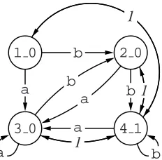
discussed in Section 2in that it allows to specify the label of the forbidden edge.2 See Figure
6for the effect ofdistinguish! on the sample automaton, where we typeset new labels in italics.
Next, the rule schemapropagatelooks for pairs of states that have not yet been discovered as distinguishable (and so are not linked by a1-edge). The states must have outgoing transitions with the same symbol, leading to states that have already been discovered as distinguishable. Again, a newly discovered pair of distinguishable states is marked by1-labelled edges with op-posite directions. The subprogrampropagate!thus implements the repeat-loop of Algorithm
1.
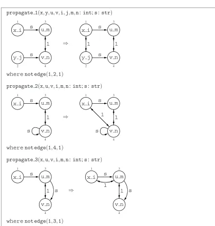
Rule schema propagate has the ‘all matches’ attribute, meaning that nodes of the schema can be merged before the schema is applied. An alternative view is thatpropagatecan be applied using non-injective graph morphisms. (See [HMP01] for details and the equivalence of both views.) For the benefit of the reader, Figure7lists the standard rule schemata represented bypropagatethat are possibly applicable to an automaton. Other schemata obtained by node merging can be ruled out because our automata do not contain1-labelled loops and do not have
1 0
3 0 4 1
2 0 b
a b
a b
a
a 1 b
1 1
Figure 6: Sample automaton afterdistinguish!
states with multiple outgoing transitions labelled with the same symbol.
Lemma1guarantees that after termination ofpropagate!, all pairs of distinguishable states have been discovered. Thus we can mark the remaining pairs as equivalent, linking their states with0-labelled edges in the subprogramequate!. The effect ofpropagate!andequate!
on the sample automaton is shown in Figure8aand Figure8b. We remark that0-edges create a structure similar to the “equivalent states layer” in the FIRE Station tool for regular language visualisation [FCW05].
4.2 Merging Phase
After termination of the macromark, the states of the input automaton are partitoned into equiv-alence classes: these are the subsets of states that are pairwise linked by0-labelled edges. Next we have to merge all the states in each partition into one state representing the partition. We need to ensure that all transitions to states that are not representing partitions are redirected to the unique states representing the partitions. Transitions outgoing from non-representative states can be removed, as can these states themselves. The merging process is implemented by the macromerge, whose rule schemata are shown in Figure9.
We first consider the partition containing the initial state. The rule schemainitmarks this state as the unique representative of its partition by adding an extra 0-tag to the state’s label. Then the loopadd tag!marks all other states in the initial partition with an extra1-tag. This marking procedure is repeated for all other partitions, by the nested loop(choose;add tag!)!. In each iteration of the outer loop, some unmarked state is chosen as the unique representative of its partition and subsequently all other states in the partition are marked as non-representative states.
After all states have been marked as representatives or non-representatives, the rule schemata
propagate 1(x,y,u,v,i,j,m,n:int;s: str) x i 1 u m 3 y j 2 v n 4 s s 1 1 ⇒ x i 1 u m 3 y j 2 v n 4 s s 1 1 1
wherenot edge(1,2,1)
propagate 2(x,u,v,i,m,n:int;s:str)
x i 1 u m 3 v n 4 s s 1 1 ⇒ x i 1 u m 3 v n 4 s s 1 1 1
wherenot edge(1,4,1)
propagate 3(x,u,v,i,m,n:int;s:str)
x i 1 u m 3 v n 4 s
1 s ⇒
x i 1 u m 3 v n 4 s 1 1 s
wherenot edge(1,3,1)
Figure 7: Rule schemata represented bypropagateusing ‘all matches’
Finally, the rule schemaclean upexhaustively applies the rule schemata shown in Figure
1 0
3 0 4 1
2 0 b a b a b a
a 1 b
1 1
1
1
(a) Afterpropagate!
1 0
3 0 4 1
2 0 b a b a b a
a 1 b
1 1 1
1
0
(b) Afterequate!
1 0 0
3 0 1 4 1
2 0 b a b a b a
a 1 b
1 1 1
1 0
(c) Afterinit;add tag!
1 0 0
3 0 1 4 1 0
2 0 0
b b b 1 1 1 1 1 0 a a a
(d) Afterredirect!
1 0 0
3 0 1 4 1 0
2 0 0
b b b a a a
(e) Afterremove edge!
1 0 4 1 2 0 b b b a a a
(f) Afteruntag!
Figure 8: Snapshots of the sample automaton
5
Correctness of the Implementation
In this section we argue that the graph program of Figure3correctly implements Algorithm1.
Lemma 2 The program of Figure3terminates for every input automaton.
init(i:int)
1 i
1
⇒ 1 i 0
1
add tag(x,y,i,j:int)
x i 0
1
y j
2
0 ⇒
x i 0
1
y j 1
2
0
choose(x,i:int)
x i
1
⇒ x i 0
1
disconnect(x,u,i,m,p:int;s:str)
u m p
2
x i 1
1
s ⇒
u m p
2
x i 1
1
all matches
redirect(x,y,u,i,j,m:int;s:str)
u m 0
2
x i 1
1
y j 0
3
s
0
⇒
u m 0
2
x i 1
1
y j 0
3
s
0
all matches
Figure 9: Rule schemata of the macromerge
of opposite direction. Similarly, each application ofequatereduces the number of state pairs that are not linked by 0-labelled edges of opposite direction. Thus the macromarkterminates.
remove edge(x,y,i,j,k,m,n:int)
x i k
1
y j m
2
n ⇒
x i k
1
y j m
2
remove node(x,i:int)
x i 1 ⇒ /0
untag(x,i:int)
x i 0
1
⇒ x i
1
Figure 10: Rule schemata of the macroclean up
a label of the form x i 1, where x and i are integers. Hence both the first loop add tag!
and the nested loop(choose; add tag!)! terminate (note that choosedoes not affect labels of the form x i 1). The loop disconnect!is trivially terminating as each application ofdisconnectreduces the number of edges in a graph. The loopredirect! terminates because each application ofredirectreduces the sum of the degrees of nodes with a label of the form x i1. Thus the macromergeterminates, too.
The termination of the three loops in the macroclean upis similarly easy to see. The rule schemata of the first two loops reduce the number of edges respectively the number of nodes, and each iteration of the loopuntag!reduces the number of nodes with three tags.
Lemma 3 The macro marklinks two distinct states by a 0-labelled edge if and only if the states are equivalent.
Proof. The loopdistinguish!implements stage 1 of the marking phase of Algorithm1in that it links final states with non-final states by a 1-labelled edge, marking such pairs as non-equivalent. Also,propagate! implements stage 2 of the marking phase: the three standard rule schemata represented bypropagate(see Figure7) cover the possible relations between the state pairs{p,q}and{δ(p,a),δ(q,a)}in the repeat-loop of Algorithm1. In particular, they cover the special cases p=δ(p,a), q=δ(q,a), p=δ(q,a) and q=δ(p,a). Hence Lemma1
implies that after termination ofpropagate!, two states are linked by a1-labelled edge if and only if they are not equivalent. The loopequate!then links two distinct states by a0-labelled edge if and only if they are not linked by a1-labelled edge, implying the proposition.
Proof. Consider an equivalence class of states of the input automaton. Exactly one state in this class is selected either by the rule schema init(in the case of the initial state’s class) or by the rule schemachoose (in all other cases), and a 0-tag is appended to the state’s la-bel. Then the loop add tag! marks all other states in the equivalence class with an extra
1-tag. Subsequently,disconnect!removes all transitions outgoing from1-tagged states and
redirect!redirects away all transitions leading to1-tagged states. Hence, after termination of the macro merge, 1-tagged states can be incident only to edges labelled with0 or1. All these edges are deleted by the loopremove edge!, so the1-tagged states become isolated and are eventually removed byremove node!. Thus, upon termination of the macroclean up, from each equivalence class exactly one state remains in the resulting automaton.
Theorem 2 For every input automaton A, the automaton ˆA produced by the program of Figure
3is equivalent to A and minimal.
Proof. By Theorem1, Lemma2and Lemma3, it suffices to show that the subprogrammerge; clean upcorrectly implements the merging phase of Algorithm1. This can be seen as follows:
• By Lemma4, each equivalence class of A is represented by its unique representative ele-ment in ˆA.
• The rule schemainitselects the initial state of A as the representative of its class and
untagmakes this state the initial state of ˆA.
• Consider any equivalence class of states X , its representative p∈X and any a∈Σ. If δ(p,a) is the representative of its equivalence class, then both states are marked with a 0-tag in mergeand the transition from p to δ(p,a) is preserved by the subprogram disconnect!;redirect!. Otherwise, if δ(p,a) does not represent its class, then it is marked with a1-tag in merge. In this caseredirect! redirects the transition p→ δ(p,a)to the unique representative of the class ofδ(p,a). Hence ˆδ(X,a), the equivalence class ofδ(p,a), does not depend on the choice of p and thus is well-defined.
• In an equivalence class containing a final state, all states are final as otherwise the loop
distinguish!would have linked the non-final states with the final state by1-labelled edges. Hence the representative of such a class is a final state.
6
Time Complexity
In this section we establish an upper bound for the number of rule schema applications of the minimization program, in terms of the size of the input automaton. This provides a worst-case estimate for the running time of our program, where we abstract from the cost of rule schema matching.3
As before, letΣbe the alphabet of an input automaton and Q its set of states. We show that each loop in the program of Figure3terminates after at most|Q|2or|Σ| · |Q|rule schema applications. In the following lemmata, n always refers to the number of states (nodes) in an input automaton. Our proofs tacitly rely on the fact that none of the rule schemata of the minimization program increases the number of nodes in a graph.
Lemma 5 The loopsdistinguish!,propagate! and equate! each terminate after at most n2rule schema applications.
Proof. Given a graph X , let #X be the number of pairshu,viof nodes such that there is no edge with label 1 from u to v. Then #X≤n2and for every step G→
distinguishH and G→propagateH,
we have #G>#H. This implies the claim for distinguish! and propagate!. The same argument works forequate! if we redefine #X as the number of pairshu,visuch that there is no edge with label 0 from u to v.
Lemma 6 The loopsadd tag! and(choose;add tag!)! each terminate after at most n rule schema applications.
Proof. Given a graph X , let #X be the number of nodes with a label of the form i j, where i and j are integers. Then #X ≤n and every step G→add tagH and G→chooseH satisfies #G>#H.
This implies the claim.
The complexity of the loops for disconnecting nodes and redirecting edges depends not only on the number of nodes (states) but also on the size of the alphabetΣ.
Lemma 7 The loops disconnect! and redirect! each terminate after at most|Σ| ·n rule schema applications.
Proof. Each node of an input automaton has|Σ|outgoing edges labelled with symbols from Σ (represented as strings), and no rule schema removes or creates such edges beforedisconnect! is executed. Hencedisconnect! terminates after|Σ| ·n rule schema applications.
Given a graph X , let #X be the number ofΣ-labelled edges whose target nodes have labels of the form i j 1 for some integers i and j. Then #X≤ |Σ| ·n and every step G→redirectH satisfies
#G>#H. Henceredirect! terminates after at most|Σ| ·n rule schema applications.
Lemma 8 The loopremove edge! terminates after at most n2rule schema applications.
Proof. The following invariant of the minimization program is easy to prove: in each graph of a computation, each pair of distinct nodes is connected by at most one pair of opposite edges labelled with 1 or 0. (Note that an input automaton does not possess such edges.) This invariant clearly implies the claim.
Lemma 9 The loops remove node! anduntag! each terminate after at most n rule schema applications.
that every step G→untagH reduces the number of nodes labelled i j k for some integers i, j and
k.
Summarising the above lemmata, we can see that the number of rule schema applications used by the minimization program is quadratic in the size of the input automaton.
Theorem 3 The program of Figure3terminates after at most O(|Q|2+|Σ| · |Q|)rule schema applications.
7
Conclusion
We have shown how to minimize finite automata with rule-based, visual programming. Program-mers need not be concerned with low-level data structures such as state tables but can directly manipulate the transition diagrams of automata. Moreover, GP’s rule schemata and control con-structs provide a convenient language for reasoning about the correctness and the complexity of the implementation. Last but not least, theall matchesoption for rule schemata has proved to be useful for keeping the number of rule schemata small, and an extendededgepredicate has been crucial for forbidding particular edges in the conditions of rule schemata.
The macromergemerges equivalent states by choosing representatives of equivalence classes, removing and redirecting transitions, and removing isolated states. A simpler implementation would use non-injective rule schemata to merge states directly—but such rule schemata are not available in GP. Non-injective rule schemata are also useful in other applications and may be realised in a future version of GP.
Finally, this case study could be extended by implementing more efficient automata mini-mization algorithms. We chose the algorithm of Hopcroft, Motwani and Ullman because of its simplicity, but its cubic running time is not optimal. More efficient algorithms include the quadratic algorithm of Hopcroft and Ullman [HU79] and Hopcroft’s nlogn algorithm [Hop71].
Acknowledgements: We are grateful for the comments of the anonymous referees which helped to improve the presentation of this paper.
Bibliography
[FCW05] M. Frishert, L. G. Cleophas, B. W. Watson. FIRE Station: An Environment for Ma-nipulating Finite Automata and Regular Expression Views. In Implementation and Application of Automata (CIAA 2004), Revised Selected Papers. Lecture Notes in Computer Science 3317, pp. 125–133. Springer-Verlag, 2005.
[HMP01] A. Habel, J. M ¨uller, D. Plump. Double-Pushout Graph Transformation Revisited. Mathematical Structures in Computer Science 11(5):637–688, 2001.
[Hop71] J. E. Hopcroft. An nlogn algorithm for minimizing the states in a finite automaton. In Kohavi (ed.), The Theory of Machines and Computations. Pp. 189–196. Academic Press, 1971.
[HP02] A. Habel, D. Plump. Relabelling in Graph Transformation. In Proc. International Conference on Graph Transformation (ICGT 2002). Lecture Notes in Computer Sci-ence 2505, pp. 135–147. Springer-Verlag, 2002.
[HU79] J. E. Hopcroft, J. D. Ullman. Introduction to Automata Theory, Languages, and Com-putation. Addison-Wesley, 1979.
[MP08] G. Manning, D. Plump. The GP Programming System. In Proc. Graph Transforma-tion and Visual Modelling Techniques (GT-VMT 2008). Electronic CommunicaTransforma-tions of the EASST 10. 2008.
[Plu09] D. Plump. The Graph Programming Language GP. In Proc. Algebraic Informatics (CAI 2009). Lecture Notes in Computer Science 5725, pp. 99–122. Springer-Verlag, 2009.
[PS10] D. Plump, S. Steinert. The Semantics of Graph Programs. In Proc. Rule-Based Programming (RULE 2009). Electronic Proceedings in Theoretical Computer Sci-ence 21, pp. 27–38. 2010.
[PSS10] D. Plump, R. Suri, A. Singh. Minimizing Finite Automata with Graph Programs. In Proc. Graph Computation Models (GCM 2010). CTIT Workshop Proceedings WP 2010-05, pp. 97–110. University of Twente, 2010.