6
PART II THE MARKET SYSTEM
Household Behavior
and Consumer Choice
Household Choice in Output Markets
Every household must make three basic decisions:
1. How much of each product, or output, to demand
2. How much labor to supply
Household Choice in Output Markets
The Determinants of Household Demand
Several factors influence the quantity of a given good or service demanded by a single household:
The price of the product
The income available to the household
The household’s amount of accumulated wealth
The prices of other products available to the household
The household’s tastes and preferencesTABLE 6.1 Possible Budget Choices of a Person Earning $1,000 Per Month After Taxes
Option
Monthly
Rent Food
Other Expense
s
Total Available ? A $ 400 $250 $350 $1,000 Yes B 600 200 200 1,000 Yes C 700 150 150 1,000 Yes
D 1,000 100 100 1,200 No
Household Choice in Output Markets
The Budget Constraint
budget constraint The limits imposed on household choices by income, wealth, and product prices.
Household Choice in Output Markets
Preferences, Tastes, Trade-Offs, and Opportunity Cost
FIGURE 6.1 Budget Constraint and Opportunity Set for Ann and Tom
A budget constraint separates those combinations of goods and services that are available, given limited income, from those that are not. The available combinations make up the opportunity set.
real income refers to the amount of goods and
HOUSEHOLD CHOICE IN OUTPUT MARKETS
The Equation Of The Budget Constraint
In general, the budget constraint can be written:
+ P
YY
where PX = the price of X, X = the quantity of X consumed, PY = the price of Y, Y = the quantity of Y consumed, and I = household income.
HOUSEHOLD CHOICE IN OUTPUT MARKETS
Budget Constraints Change When Prices Rise or Fall
FIGURE 6.2 The Effect of a Decrease in Price on Ann and Tom’s Budget Constraint
When the price of a good
Basic Model of Rational Choice
•
The consumer choice model contains three essential
elements:
•
Preferences
- what the consumer wants to do
•
Budget constraint
- what the consumer can afford to do
•
Consumer equilibrium
- the rational choice given the consumer's
preferences and budget constraint - the choice that maximizes
benefit subject to the budget constraint
Basic Model of Rational Choice
• Preferences
The consumer is assumed to have preferences over different combinations (bundles) of goods which obey certain basic "rules" (axioms).
• Axioms
There are three fundamental assumptions concerning individual preferences:
• Completeness - given any two bundles A and B the individual either prefers A to B, B to A, or is indifferent between them
• Consistency (Transitivity) - given any three bundles A, B and C, if A is preferred to B and B to C then A must be preferred to C.
The Basis of Choice: Utility
utility The satisfaction, or reward, a product yields relative to its alternatives. The basis of choice.
marginal utility (MU) The additional satisfaction gained by the consumption or use of one more unit of something.
Diminishing Marginal Utility
total utility The total amount of satisfaction obtained from consumption of a good or service.
The Basis of Choice: Utility
•
Ordinal Utility Function
In order to rank bundles according to a consumer's preferences an arbitrary number is assigned to each bundle. U(A) indicates the utility of bundle A. These numbers comprise an ordinal utility function with the following properties:
• If U(A) > U(B) then A is preferred to B.
• If U(A) = U(B) then the consumer is indifferent between bundles A and B
TABLE 6.2 Total Utility and Marginal Utility of Trips to the Club Per Week
Trips to Club Total Utility Marginal Utility
1 12 12
2 22 10
3 28 6
4 32 4
12
The Basis of Choice: Utility
FIGURE 6.3 Graphs of Frank’s Total and Marginal Utility
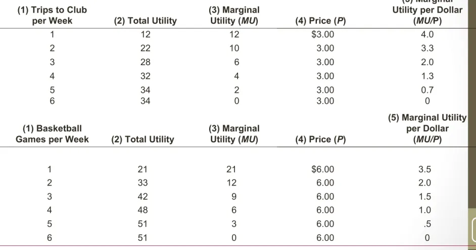
TABLE 6.3 Allocation of Fixed Expenditure per Week Between Two Alternatives
(1) Trips to Club
per Week (2) Total Utility
(3) Marginal
Utility (MU) (4) Price (P)
(5) Marginal Utility per Dollar
(MU/P)
1 12 12 $3.00 4.0
2 22 10 3.00 3.3
3 28 6 3.00 2.0
4 32 4 3.00 1.3
5 34 2 3.00 0.7
6 34 0 3.00 0
(1) Basketball
Games per Week (2) Total Utility
(3) Marginal
Utility (MU) (4) Price (P)
(5) Marginal Utility per Dollar
(MU/P)
1 21 21 $6.00 3.5
The Basis of Choice: Utility
Allocating Income To Maximize Utility
(4) Price (P)
(5) Marginal Utility per Dollar
(MU/P)
$3.00 4.0 3.00 3.3 3.00 2.0 3.00 1.3 3.00 0.7 3.00 0
(4) Price (P)
(5) Marginal Utility per Dollar
(MU/P)
The Basis of Choice: Utility
The Utility-Maximizing Rule
In general, utility-maximizing consumers spread out their expenditures until the following condition holds:
utility-maximizing rule:
XY
for all goods
X Y
MU
MU
P
P
utility-maximizing rule Equating the ratio of the marginal utility of a good to its price for all goods.
The Basis of Choice: Utility
Diminishing Marginal Utility and Downward-Sloping Demand
FIGURE 6.4 Diminishing Marginal Utility and Downward-Sloping Demand
The more of a good consumed the less marginal (extra) utility
Income and Substitution Effects
The Income Effect
Price changes affect households in two ways. First, if we assume that households confine their choices to products that improve their well-being, then a decline in the price of any product, ceteris paribus, will make the household unequivocally better off.
In other words, if a household continues to buy the same amount of every good and service after the price decrease, it will have income left over. That extra income may be spent on the product whose price has declined, hereafter called good X, or on other products.
Income and Substitution Effects
The Substitution Effect
When the price of a product falls, that product also becomes relatively cheaper. That is, it becomes more attractive relative to potential substitutes. A fall in the price of product X might cause a household to shift its purchasing pattern away from substitutes toward X. This shift is called the substitution effect of a price change.
Everything works in the opposite direction when a price rises, ceteris paribus. When the price of a product rises, that item
18
Income and Substitution Effects
FIGURE 6.4 Diminishing Marginal Utility and Downward-Sloping Demand
Appendix
We base the following analysis on four assumptions:
1. We assume that this analysis is restricted to goods that yield positive marginal utility, or, more simply, that “more is better.”
(Non-satiation)
2. The marginal rate of substitution is defined as MUX/MUY, or the ratio at which a household is willing to substitute X for Y. We assume a diminishing marginal rate of substitution.
3. We assume that consumers have the ability to choose among the combinations of goods and services available (Completeness)
4. We assume that consumer choices are consistent with a simple
INDIFFERENCE CURVES
Consumer surplus
•
An individual buys a good only if the purchase is expected to
make the person better off (or at least no worse off).
•
In general, the total benefit received from the purchase of a
commodity is expected to exceed the opportunity cost.
•
This provides consumers with a net gain from trade, referred to
as consumer surplus
.
Consumer surplus
•
Suppose that an individual buys 10 units of a good at a price of
$5.
As the diagram below indicates, the first unit of this good costs $5, but this individual would have been willing to pay a price of up to $9 for this first unit of this good. In this case, the
consumer receives a good that he or she values at $9 by giving up only $5. Thus, the first unit of the good
22 of
Generally, the total benefit from consuming 10 units of this good is the entire area under the demand curve (as illustrated by the blue shaded area in the diagram below).
The total cost of
Consumer surplus
The consumer surplus received by this
consumer is the
difference between the total benefit and total cost. This is
represented by the red shaded area in the diagram below. As noted above, the consumer surplus represents the
DERIVING INDIFFERENCE CURVES
An Indifference Curve
An indifference curve is a set of points, each representing a combination of some amount of good X and some amount of good Y, that all yield the same amount of total utility.
The consumer depicted here is indifferent between bundles A
A Preference Map: A Family of Indifference Curves
Each consumer has a unique family of indifference curves called a
preference map. Higher indifference curves represent higher levels of total utility.
PROPERTIES OF INDIFFERENCE CURVES
)
(
MU
Y
X
MU
X
Y
Y X MU MU X Y
1. Negatively- Sloped - - this follows from the assumption of non-satiation.
•
Convex to the origin
- this property results from the
assumption that the MRS
diminishes
as we move along an
indifference curve.
26 of
•
More utility the further from the origin
- because of
non-satiation, indifference curves further from the origin (with
more of both goods) must represent higher levels of utility.
(See diagram above where U2 > U1)
•
Cannot intersect
- the axiom of transitivity implies that
indifference curves cannot intersect each other.
Y X Y X P P MU
MU
CONSUMER CHOICE
At point B:
Consumer Utility- Maximizing Equilibrium
Consumers will choose the combination of X and Y that maximizes total utility.
Graphically, the consumer will move along the budget constraint until the highest possible indifference curve is reached. At that point, the budget constraint and the indifference curve are tangent. This point of tangency occurs at X* and Y* (point B).
Y
X
MU
DERIVING A DEMAND CURVE FROM INDIFFERENCE CURVES AND BUDGET CONSTRAINTS
Budget constraint Opportunity set Real income Utility
Marginal utility
Law of diminishing marginal utility
REVIEW TERMS AND CONCEPTS
Utility maximizing rule
Income and substitution effects Indifference curve