¨
Ozye˘gin University Spring 2020
CS480/CS580 Quantum Computing
Lecture 2 - Mathematical Background
17.02.2020Scribe: Furkan Kınlı - Arman Hasanzade Lecturer: ¨Ozlem Salehi K¨oken
2
Mathematical Background
In this manuscript, it is explained some necessary mathematical background to deeply un-derstand quantum systems. First, classical systems will be explained, and then probabilistic systems and quantum systems will be investigated.
2.1
Classical Systems
We start our discussion with classical bits and clasical systems. 2.1.1 Basics, Vector Representation
Bit: Smallest unit of information used in classical computers. A bit (binary digit) can be any object with two states (e.g. the light on/off) and these two states are generally represented by 0 and 1. It is not important what actually realizes it.
Note: 1 bit represents two states. Q: Why binary?
A: Because it is more efficient, and easy to use a system with two different levels rather than d levels. Computers working with 2 levels are easier to work with. Generally this is represented by 5 Volts.
Representation of bit as a vector
We can represent this information (i.e. a single bit) using vector representation, and need a 2-dimensional vector to represent a single bit since it has 2 distinct states.
0 =
1 0
,1 =
0 1
2.1.2 Operations on a Single Bit
The operations that can be perform on a single bit are as follows:
1. NOT operation maps 0 to 1 and 1 to 0. In other words, it maps x to ¬x where x∈ {0,1}.
NOT: 0 → 1 NOT: 1 → 0
We can use the following table representation for the NOT operator:
P P
P P
P P
P PP
Final
Initial
0 1
0 0 1
1 1 0
The first row represents the initial values and the first column represents the final values. Since we are considering the NOT operation, when given an input of 0, it is mapped to 1, and we can see the corresponding matrix cell for initial state of 0 and final state of 1 (3rd row, 2nd col) is marked as 1. If we consider initial state of 0 and final state of 0, we see that the corresponding cell is marked as 0.
In summary, the cell corresponding to (i, j) is 1 if iis mapped to j, and 0 otherwise. 2. IDENTITY (I) operator maps both 0 and 0 to 1 to 1.
I: 0 →0 I: 1 →1 Its corresponding table is as follows:
P P
P P
P P
P PP
Final
Initial
0 1
0 1 0
1 0 1
Its corresponding table is as follows:
P P
P P
P P
P PP
Final
Initial
0 1
0 1 1
1 0 0
4. ONE operator maps both 0 and 1 to 1
ONE: 0 → 0 ONE: 1 → 1 Its corresponding table is as follows:
P PP
P P
P P
PP
Final
Initial
0 1
0 0 0
1 1 1
Table representation of the states gives a matrix formulation of the operations. We can trace the evolution of a bit using these linear operations.
Example:
0=
1 0
and 1 =
0 1
0 1 1 0
1 0
=
0 1
Not operation applied to state 0 gives us 1. In other words NOT(0) = 1. Q: Can we guess the input from the output?
A: In case of the NOT operation we can, but this is not always the case. This property is called Reversibility.
Note that NOT and IDENTITY are reversible, whereas ZERO and ONE are not re-versible operators. Being rere-versible means that it is possible to recover the input. We will see that in quantum computing, all operations must be reversible.
2.2
Probabilistic Systems
Main motivation in defining classical and probabilistic systems is that understanding these systems leads to consider that quantum systems are the generalization of probabilistic tems. Also, probabilistic systems can be referred as the generalization of the classical sys-tems.
2.2.1 Basics, Vector Representation
Let’s consider a fair coin where head represents 0, and tail 1. In fact, a coin represents two states as in classical systems. Suppose that we flip the coin. Until observing the outcome, it basically represents a probabilistic system where P(0) =P(1) = 0.5.
Our knowledge about the coin can represented by a 2-dimensional vector that refers the probability of observing 0 or 1 (i.e. being in state 0 or state 1):
P(0) P(1)
=
0.5 0.5
Example:
If the coin is biased, sayP(0)/P(1) = 3, it can be represented with the following vector:
P(0) P(1)
=
0.75 0.25
Based on the above observations, we can conclude that any vector v =
a b
where a+b= 1, a, b≥0 represents a probabilistic system. Note thatkvk1 = 1 where k k1 denotes the L1 norm and such vectors with nonnegative entries are called stochastic vectors.
2.2.2 Probabilistic operators
What operators can we apply to probabilistic bits? Such an operator should take a proba-bilistic state as input, and transforms it into another probaproba-bilistic state. The input cannot contain any non-negative value since it represents the probability, and the column should add up to 1. Besides, the output vector should also a stochastic vector to represent a prob-abilistic system.
Fair Coin
P P
P PP
P P
PP
Final
Initial
0 1
0 12 12
1 12 12
Biased Coin
P P
P P
P P
P PP
Final
Initial
0 1
0 34 34
1 14 14
Further reading about the subject: Markov chains
Example:
Suppose that we have 2 coins,
• Euro with [H :T] = 3 : 2
• Cent with [H :T] = 3 : 7
For Euro ⇒ P(H) = 0.6 and P(T) = 0.4
For Cent ⇒ P(H) = 0.3 andP(T) = 0.7
Start with one Euro, flip it. If it is heads, flip Euro again. If it is tails, flip the Cent.
The probability table evolving the system is given by: (Note that 0 is H, and 1 is T)
P P
P P
P P
P PP
Final
Initial
0 1
0 0.6 0.3
1 0.4 0.7
We can use the table to represent the coin flip as matrix multiplication and trace the evolution of the system.
After 1st flip with Euro the state of the system is represented with the following vector:
0.6 0.3 0.4 0.7
1 0
=
0.6 0.4
After the second flip, the state of the system is represented with the following vector:
0.6 0.3 0.4 0.7
0.6 0.4
=
0.36 + 0.12 0.24 + 0.28
=
HH +T H HT +T T
=
0.48 0.52
We observe that columns of the matrices corresponding to probabilistic operators should be stochastic. Such matrices are called stochastic matrices. Note that the output obtained after multiplying a stochastic matrix with a stochastic vector is also a stochastic vector, whose column adds up to 1, and entries are non-negative. We can conclude that any stochastic matrix is a probabilistic operator.
Note that if an operator is reversible, then the corresponding matrix should be invertible. It turns out that if a stochastic matrix is invertible, then it must be a permutation matrix, in which case the system is evolves deterministically. Note that its inverse should also be a stochastic matrix since otherwise it wouldn’t be able to preserve the length of the vector. This makes sense as we are not able to guess the input when the operator maps the current state to a probabilistic state.
2.3
Multiple Bits
So far we have discussed single bits and probabilistic bits. Now we will talk about systems having more than one bit.
2.3.1 Notation
To represent multiple bits we will introduce a new notation. This notation is basically the foundation of the notation in quantum systems.
Let’s use [0] =
1 0
and [1] =
0 1
to represent the states 0 and 1, respectively. At this point, any probabilistic state
a b
can be represented as follows:
a b
=a
1 0
+b
0 1
=a[0] +b[1]
This notation is particularly useful when we have more than 1 bit (2 states). Representing two bits
Q:Suppose that we have 2 probabilistic bits, how many different states can be represented?
• [00]: Both bits are in state 0.
• [01]: The first bit is in state 0, the second one is in state 1.
• [10]: The first bit is in state 1, the second one is in state 0.
• [11]: Both bits are in state 1.
If we have two bits, then the combined system has four basis states. Any probabilistic state with two probabilistic bits can be expressed as the linear combination of these basis states. Mathematically speaking, this mechanism refers to a term called Tensor Product.
2.3.2 Tensor Product
Tensor product is a way of combining spaces, vectors, or operators together. In other words, the Tensor product is a way of putting vector spaces together to form larger vector spaces. We use this property to combine two systems together.
Tensor product properties:
• Tensor product distributes over addition in the same way as the distribution of multi-plication over addition.
Example:
Suppose that we have 2 probabilistic bits represented by the vectors x= 0.2[0] + 0.8[1]
y = 0.6[0] + 0.4[1]. The states of combined system is given follows:
x⊗y= (0.2[0] + 0.8[1])⊗(0.6[0] + 0.4[1]) = 0.12[00] + 0.08[01] + 0.48[10] + 0.32[11] We can read the probability of each state by looking at the coefficients. Tensor product of vectors:
Let’s say a=
a0
a1
and b =
b0
b1
, then
a⊗b =
a0 a1 ⊗ b0 b1 = a0 b0 b1 a1 b0 b1 =
a0b0
a0b1
a1b0
a1b1
.
2.3.3 Vector Representation of Combined Systems
This representation can be extracted by applying tensor product to the vectors of subsystems. For 2-bit cases, vector representations of the combined systems are calculated as follows:
• Both bits are in state 0.
[00] = [0]⊗[0]
= 1 0 ⊗ 1 0 = 1 0 0 0
• The first bit is in state 0, the second one is in state 1. [01] = [0]⊗[1]
= 1 0 ⊗ 0 1 = 0 1 0 0
• The first bit is in state 1, the second one is in state 0. [10] = [1]⊗[0]
= 0 1 ⊗ 1 0 = 0 0 1 0
• Both bits are in state 1.
[11] = [1]⊗[1]
= 0 1 ⊗ 0 1 = 0 0 0 1
We can infer that a vector of dimension 4 is needed to represent any combined systems with 2-bits. These are called basis states for 2-bits systems, and any probabilistic system with 4 states can be expressed with these aforementioned states.
Example:
From the previous example, recall that the state of the combined system is 0.12[00] + 0.08[01] + 0.48[10] + 0.32[11].
The same state can be equivalently expressed as
0.12 1 0 0 0 + 0.08 0 1 0 0 + 0.48 0 0 1 0 + 0.32 0 0 0 1 = 0.12 0.08 0.48 0.32
Alternatively, we can calculate the vector of the combined system by applying tensor product to the state vectors of the subsystems. The final state representation will be exactly the same.
a⊗b=
0.2 0.8
⊗
0.6 0.4
=
0.12 0.08 0.48 0.32
Q:Suppose that we haveN-bits. How many different states can be represented withN-bits? A: N-bits can represent 2N different states. In such a case, the dimension of the vectors
representing this combined system will be 2N. After a certain point, it becomes very hard to work with N-dimensional vectors. Instead, with the help of this notation (e.g. [00], [10] etc.), we can represent such a system with N bits by using onlyN numbers, and it becomes easier to follow.
2.3.4 Operations on Multiple Qubits
Tensor product of matrices: In previous cases, we used tensor product to combine states of systems. Additionally, we can use it to combine operators. Considering that a particular operator is applied on the first bit, and another operator on the second bit, then this means that we can apply tensor of two operators on the combined system.
Given two matrices A and B, their tensor product is defined as
A ⊗ B =
a11B a12B . . . a1nB
..
. . .. ...
a1mB am2B . . . amnB
where aij is the entry in row icolumn j of matrix A.
Example:
Suppose that we have 2 bits and we apply NOT operator on the first bit. What is the combined operator applied on 2 bits?
Since we do not change the second bit, we can apply IDENTITY operator to the second bit. Tensor product of NOT and I is the combined operator for this case, and formed as follows:
0 1 1 0
⊗
1 0 0 1
=
0 0 1 0 0 0 0 1 1 0 0 0 0 1 0 0
Initially let’s assume that both bits are in state 0. Applying NOT operator on the first bit leads to change the system to [10], which means the first bit is in state 1, the second bit is in state 0. This can be doubled checked by performing the following matrix vector multiplication:
0 0 1 0 0 0 0 1 1 0 0 0 0 1 0 0
1 0 0 0
=
0 0 1 0
2.3.5 More Than Two Bits
When we have n bits, then the basis states are of the form [a1 ... an] where ai ∈ {0,1}
and such a system is described by a 2n-dimensional vector. Sometimes, it is easier to work
with the state notation, and sometimes, it might be easier to work with the vectors and matrices. In fact, when simulating a quantum computer in a classical computer, we compute the state vector, and evolve it by making matrix multiplications. This process is costly since to simulate such a system with n qubits, 2n-dimensional matrix-vector multiplication
2.4
Quantum Systems
In this section we will talk about the basics of quantum systems. Before going into the details of mathematical background, we start with two experiments to get some motivation.
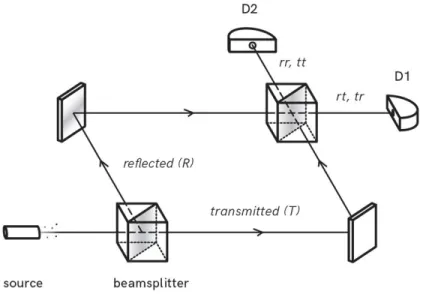
Figure 1: Experiment with a single beam splitter
In Figure 1, the beam splitter can be considered as the flip of a coin as it is observed that both detectors have 12 chance to receive the beam.
Figure 2: Experiment with two beam splitters
Thinking beamsplitter as a coin flip, we might again guess that both detectors have 12 chance to receive the photon in Figure 2. However, the experimental results show that the photon is received by detector D2 with probability 1 and by D1 with probability 0.
2.4.1 Background on Linear Algebra
In this section we will make some necessary definition for the mathematical background of quantum systems.
Vector space: A vector space V is a set that is closed under vector addition and scalar multiplication. Elements of a vector space are called vectors and we use the column vector notation to indicate a vector.
Addition:
z1
.. . zn
+
z01 .. . zn0
=
z1+z01
.. . zn+z0n
Scalar multiplication: c
z1
.. . zn
=
cz1
.. . czn
We wlil be interested in Cn, the space of all n-tuples of complex numbers.
Dirac notation: Quantum mathematical notation for a vector in vector space. |ψi: where ψ is the label of the vector and| i is calledket.
A spanning set for a vector space is a set of vectors |v1i. . .|vni such that any vector
|vi in the vector space can be written as a linear combination |vi=P
ai|vii
A set of linearly independent vectors which span the vector space is called abasis. Num-ber of elements in basis is the dimension of V.
An inner product is a function which takes as an input two vectors|vi and|wi from a vector space and produces a complex number. The notation for inner product is (|vi, |wi)
Inner product satisfies the following properties:
1. Linearity in the second argument (|vi, P
iλi|wi) = P
iλi (|vi, |wii)
2. Conjugate-commutativity (Complex conjugate is shown by *) (|vi, |wi) = (|wi,|vi)*
3. Non-negativity
(|vi, |vi)≥ 0 with equality iff v = 0 is the zero vector.
More detailed explanation and some example for the above properties can be found in the ”Linear Algebra and the Dirac Notation PDF on LMS”
Example: Cn has inner product defined by dot product.
Considering the following vectors:
y1
.. . yn
and
z1
.. . zn
we can perform dot product as
y1∗ . . . y∗n ·
z1
.. . zn
=
P iy
∗ izi
New notation for inner product: (|vi, |wi) :=hv|wi
hv| is called the dual of vector |vi. It turns out that hv| = v1∗ . . . vn∗ that is the transpose vector of the complex conjugate of the column vector v, v†.
This is called the braket notation: h | →bra | i →ket
Vectors |viand |wi areorthogonal if hv|wi= 0. Normis defined as k |vi k =phv|vi. A vector is called a unit vector if k |vi k = 1. A set of vectors is called orthonormal if each vector in the set is a unit vector and each vector is orthogonal to an other.
Delta Kronecker notation: δij = (
0 iff i and j are different 1 otherwise
Note that hi|ji =δij.
Hilbert space: The vector spaces we consider will be over the complex numbers, and are finite-dimensional, which significantly simplifies the mathematics we need. Such vector spaces are members of a class of vector spaces called Hilbert spaces. Hilbert spaces are denoted by H and are also inner product spaces.
A linear operator on a vector space H is a linear transformation T : H → H of the vector space to itself (i.e. it is a linear transformation which maps vectors in H to vectors inH).
A(P
iαi|vii) = P
iαiA(|vii).
For every linear operator we have a matrix and every matrix has its corresponding linear operator.
Outer product: (|wihv|) (|v0i) = |wihv|v0i =hv|v0i|wi
Note that the first entry (ket bra) is the outer product and the second entry is a quantum vector. Outer product defines a matrix.
The conjugate transpose of a matrix A, denoted by A† = ¯AT where the entries of ¯A
are the complex conjugate of the corresponding entries in A.
Example:
A =
3 + 7i 0 2i 4−i
A† =
3−7i −2i 0 4 +i
Some properties:
• (A†)† = A
• (A+B)† =A†+B†
• (kA)† = ¯kA†
• (AB)† = B†A†
If A−1 =A∗, then A is called unitary. Any quantum operator should be unitary.
Example:
A= 1 2
1 +i 1−i 1−i 1 +i
AA†= 1 4
1 +i 1−i 1−i 1 +i
1−i 1 +i 1 +i 1−i
= 1 4
4 0 0 4
=
1 0 0 1
=I
Thus A is unitary.
An n×n complex matrix is unitary iff its column (also true for row) vectors form an orthonormal set.
Example: v1 = 12
1 +i 1−i
v2 = 12
1−i 1 +i
1−i
2 1+i
2
·
1+i
2 1−i
2
= 12 + 12 = 1 ⇒ hv1|v2i = 1
hv1|v2i = 0