Sharif University of Technology
Scientia IranicaTransactions B: Mechanical Engineering www.scientiairanica.com
A novel computational framework to approximate the
analytical solution of a nonlinear fractional elastic beam
equation
K. Sayevand
and K. Pichaghchi
Faculty of Mathematical Sciences, University of Malayer, Malayer, P.O. Box 16846-13114, Iran. Received 15 November 2014; received in revised form 9 February 2015; accepted 4 May 2015
KEYWORDS Caputo fractional derivative; Nonlinear elastic beam equation; Fourier transform; Laplace transform; Homotopy
perturbation method.
Abstract. In this paper, the generalized travelling solutions of the nonlinear fractional beam equation is investigated by means of the homotopy perturbation method. The fractional derivative is described in the Caputo sense. The reliability and potential of the proposed approach, which is based on joint Fourier-Laplace transforms and the homotopy perturbation method, will be discussed. The solutions can be approximated via an analytical series solution. Moreover, the convergence and stability of the proposed approach for this equation is investigated, and the results reveal that the proposed scheme is very eective and promising.
© 2016 Sharif University of Technology. All rights reserved.
1. Introduction
Many partial dierential equations are widely used to describe important phenomena in mathematics, physics and engineering [1,2]. In recent years, it has been discovered that dierential equations involving derivatives of a non-integer order can be adequate models for various physical phenomena [3-10]. The present paper is a study on developing a fairly complete theoretical understanding of the solutions for beam equations with fractional coordinate derivatives. In the nonlinear elastic beam theory, the stress in the lateral direction is neglected, and governing equations can be considered in the following form, when is the deection of the beam, and a and b are parameters:
@(x; t)
@t +
@(x; t)
@x +a
@(x; t)
@x +b(x; t)+n(x; t)=0;
(1)
*. Corresponding author. Tel./Fax: +98 8133340867 E-mail addresses: [email protected] (K. Sayevand); [email protected]. (K. Pichaghchi)
where:
0 < ; 2; 0 < 4;
a; b 2 R; n 2 N: (2) This problem has many applications in engineering systems. Some of these applications are vibrations that occur in bridges and rail-road tracks due to moving vehicles, vibrations that occur in pipe systems due to uid ow, machining operations, machine chains and belt drives, and thermal processing subjected to moving heat sources.
In this paper, we aim to establish application of the homotopy perturbation method to derive solutions for mathematical variants of the fractional beam equa-tion. The homotopy perturbation method [4,5,11-13] was rst proposed by Prof. He in order to solve various nonlinear problems [11]. This promising analytic technique has successfully been applied to solving many types of linear and nonlinear functional equations. The homotopy perturbation method, in contrast to the traditional perturbation method, does not require a small parameter and is constructed with an embedding
parameter, p 2 [0; 1], which is considered a small pa-rameter. Considerable research work has recently been conducted in application of this method to fractional advection-dispersion equations, multi-order fractional dierential equations, Navier-Stokes equations, nonlin-ear Schrodinger equations, Volterra integro-dierential equations, nonlinear oscillators, boundary value prob-lems, fractional KdV equations, quadratic Riccati dif-ferential equations of fractional order and many others. For more details about the homotopy perturbation method and its applications, the reader is advised to consult the results of research work presented in [14-19]. All these successful applications veried the eectiveness, exibility, and validity of the homotopy perturbation method.
The paper is organized as follows. After a short background on fractional calculus and mathematical prerequisites, the nonlinear fractional beam equation is investigated by means of joint Fourier-Laplace trans-forms and the homotopy perturbation method. A short summary with discussion is given in the nal section.
2. Mathematical prerequisites
Denitions of the well-known Fourier and Laplace transforms of function (x; t) and their inverses are described below [20]:
Denition 1. The Laplace transform of function (x; t) (continuous or partially continuous and of exponen-tial order as t approaches innity), with respect to t, is dened by:
Ln(x; t)o= ~(x; s) = Z 1
0 e
st(x; t)dt;
(t > 0; x2R); (3) where Re(s) > 0, and its inverse transform, with respect to s, is given by:
L 1n~(x; s)o= (x; t) = 1
2i Z +i1
i1 e
st(x; s)ds;
(4) where is a xed real number.
Denition 2. The Fourier transform of function (x; t), with respect to x, is dened by:
Fn(x; t)o= ^(!; t)=
1
Z
1
ei!x(x; t)dx; (! > 0);
(5) and the inverse Fourier transform with respect to !, is given by the formula:
F 1n^(!; t)o= (x; t) = 1
2 Z 1
1e
i!x^(!; t)d!:
(6)
Denition 3. The Mittag-Leer function, E;(z)
with > 0, > 0, is dened by the following series representation, valid in the whole complex plane:
E;(z) = 1
X
n=0
zn
(n + ); z 2 C: (7) For = 1, we obtain the Mittag-Leer function in one parameter:
E;1(z) = 1
X
n=0
zn
(n + 1) E(z): (8) Denition 4. The general H-function is dened as the inverse Mellin transform [21]:
HP;Qm;n z(a1;A1)(aP;Ap)
(b1;B1)(bQ;BQ)
!
= 2i1 Z
C m
Q
j=1 (bj Bjs) n
Q
j=1 (1 aj+Ajs) Q
Q
j=m+1(1 bj+Bjs) P
Q
j=n+1(aj Ajs)
zsds;
(9)
where contour C runs from C i1 to C + i1, separating the poles of (bj Bjs), (j = 1; ; m),
from those of (1 aj+ Ajs), (j = 1; ; n). The
integers, m, n, P and Q, satisfy 0 m Q and 0 n P . The coecients, Aj and Bj are positive
real numbers and the complex parameters, aj and bj
are such that no poles in the integrand coincide. If:
= n X j=1 Aj P X j=n+1
Aj+ m X j=1 Bj Q X j=m+1
Bj > 0;
(10) then, the integral converges absolutely and denes the H-function in the sector jarg zj <
2.
2.1. Background on fractional derivatives There are several denitions for fractional dieren-tial equations. These denitions include Grunwald-Letnikov, Riemann-Liouville, Caputo, Weyl, Mar-chaud, Riesz, and Jumarie fractional derivatives. Here, some preliminaries and notations regarding fractional calculus are presented.
Denition 5. The Caputo fractional derivative of order is dened as:
D t(t) =
8 > > > > > > < > > > > > > : 1 (m ) Rt
0(t )m 1(m)()d;
> 0; t > 0;
m 1 < < m; m 2 N;
dm
dtm(t); = m;
(11)
is allowed to be real or even complex. In this paper, only real and positive will be considered. With this denition, a fractional derivative would be dened for a dierentiable function only [22]. Recently, to overcome this limitation and in order to deal with non-dierentiable functions, the following denitions are presented.
Denition 6. We can dene a fractional derivative in the form [23]:
D
t(t)= (m )1 d m
dtm t
Z
t0
( t)m 1(
0() ())d:
(12) For a continuous and dierentiable, , we have:
0(t) =(t0) + (t t0)0(t0) +12(t t0)200(t0)
+ + 1
(m 1)!(t t0)n 1(m 1)(t0): (13) If 0(t) is continuous but not dierentiable anywhere,
we have:
0(t) =(t0) + (t t(1+)0) ()(t0)+ (t t0) 2
(1+2)(2)(t0)
+ + (t t0)m 1
(1 + (m 1))((m 1))(t0): (14) Eq. (12) is equivalent to:
D
t(t) = (m )1 d m
dtm
Z t
t0
( t)m 1
m 1X i=0
1
i!( t0)i(i)(t0) () !
d; (15)
for a continuous and dierentiable case. Eq. (12) is equivalent to:
D
t(t) = (m )1 d m
dtm
Z t
t0
( t)m 1
m 1X i=0
( t0)i
(1 + i)(i)(t0) () !
d; (16)
for continuous and nondierentiable cases.
Denition 7. Keeping only the rst term of 0(), we
give another denition of a fractional derivative in the form [23]:
D
t(t)= (m )1 d m
dtm t
Z
t0
( t)m 1((t
0) ())d:
(17)
Hereby, can be continuous and possibly not dieren-tiable anywhere.
Denition 8. We can dene another fractional deriva-tive in the form [23]:
D
t(t) = (m )1 d m
dtm
Z t
t0
( t)m 1()d:
(18) The above denitions of a fractional derivative are introduced by the variational iteration method.
Proposition 1. The Laplace transform of the Caputo fractional derivative is given in the form:
LfD
t(x; t)g = s~(x; s) n 1
X
k=0
s k 1(k)(x; 0);
(19) where ~(x; s) denote the Laplace transform of (x; t). Proposition 2. The Fourier transform of the Caputo fractional derivative is given in the form:
FfD
x(x; t)g = (i!)^(!; t); (20)
where ^(!; t) denote the Fourier transform of (x; t). 2.2. Physical understanding of the fractional
derivative
Prof. He [24] showed that fractional dierential equa-tions can best describe discontinuous media, and the fractional order is equivalent to its fractional dimen-sions. Now, consider a plane with a fractal structure. The shortest path between two points, A and B, is not a line and we have:
dsE = kds; (21)
where dsEis the actual distance between two terminal
points, A and B, ds is the line distance between two points, is the fractal dimension, and k is a constant. Projection of the dsE into the horizontal direction
yields Cantor-like sets, and its length can be expressed as:
xAB = kxdxx; (22)
where xare the fractal dimensions of the Cantor-like
sets in the horizontal direction, and kx is a constant.
Eq. (21) means the following transform:
sE= ks: (23)
Inspired by this concept of a fractional derivative, we assume that the solution of the fractional dierential equation can be expressed in terms of E(t), and the
Mittag-Leer function plays a fundamental role in our study of fractional equations.
3. The method in action
Now, we consider Eqs. (1) and (2). By using the prop-erties of the homotopy perturbation method [11,13, 14,16,19], we have the following equation:
(1 p)(Dt(x; t) + Dt(x; t) + aD
t(x; t))
+ p(D
t(x; t) + Dx(x; t) + aDx (x; t)
+ b(x; t) + n(x; t)) = 0; (24)
where p2[0; 1]. Now, we construct the following sequ-ence:
(x; t) = 0(x; t) + p1(x; t) + p22(x; t) + : (25)
Consequently, we will have: p0: D
t0(x; t) + Dx 0(x; t) + aDx0(x; t) = 0;
(26) pi :D
t1(x; t) + Dx1(x; t) + aDx 1(x; t)
= bi 1 i 1n ;
i = 1; 2; ;
... (27)
Now, in order to nd a closed form representation of the solution in terms of i(x; t), we use the method of
joint Fourier-Laplace transforms. In the other words, if we apply the Fourier transform with respect to space variable x, then, Eq. (26) transforms into the form:
Dt ^0(!; t) + (i!)^0(!; t) + a(i!)^0(!; t) = 0;
(28) where ! is the parameter of Fourier transform. Fur-thermore, taking the Laplace transform of Eq. (28), one will set:
s~^
0(!; s) s 1^0(!; 0) s 2@ ^0(!; 0)@t
+ (i!)~^
0(!; s) + a(i!)~^0(!; s) = 0; (29)
where s is the parameter of the Laplace transform. Consequently, we obtain:
~^0(!; s) = s 1
s+ (i!)+ a(i!)^0(!; 0)
+ s 2 s+ (i!)+ a(i!)
@ ^0(!; 0)
@t : (30) Consequently one will set:
t 1E
;(ct)$L ss c; (31)
it is seen that:
^0(!; t) = E;1( ((i!)+ a(i!))t)^0(!; 0)
+ tE;2( ((i!)+ a(i!))t)@ ^0@t(!; 0): (32)
We can rewrite Eq. (32) in the following form:
^0(!; t) = ^G1(!; t)^0(!; 0) + ^G2(!; t)@ ^0(!; 0)@t ; (33)
where: ^
G1(!; t) = E;1( ((i!)+ a(i!))t); (34)
and: ^
G2(!; t) = tE;2( ((i!)+ a(i!))t): (35)
Taking the inverse Fourier transform of Eq. (33), and noticing the convolution theorem of the Fourier transform, we nd that:
0(x; t) =
Z 1
1G1(x y; t)0(y; 0)dy
+ Z 1
1G2(x y; t)
@0(y; 0)
@t dy; (36) where:
G1(x; t)=21 1
Z
1
E;1( ((i!)+a(i!))t)e i!xd!;
(37) and:
G2(x; t)=2t 1
Z
1
E;2( ((i!)+a(i!))t)e i!xd!:
(38) Now, applying the Fourier transform into Eq. (27), we have:
Dt ^1(!; t) + (i!)^1(!; t) + a(i!)^1(!; t)
= b^0(!; t) ^02(!; t): (39)
Taking the Laplace transform of Eq. (39), we nd that:
s~^
1(!; s) s 1^1(!; 0) s 2@ ^1(!; 0)@t
+ (i!)~^
1(!; s) + a(i!)u~^1(!; s)
= b~^0(!; s) ~^20(!; s); (40)
~^1(!; s) = s 1
s+ (i!)+ a(i!)^1(!; 0)
+s+ (i!)s 2+ a(i!) @ ^1@t(!; 0)
b
s+ (i!)+ a(i!)~^0(!; s)
1
s+ (i!)+ a(i!)~^02(!; s): (41)
Inverting the Laplace transform with the help of the result of Relation (31), the following is obtained:
^1(!; t) =E;1( ((i!)+ a(i!))t)^1(!; 0)
+ tE;2( ((i!)+ a(i!))t)@ ^1@t(!; 0)
b Z t
0 (t ) 1E
;( ((i!)
+ a(i!))(t ))^
0(!; )d
Z t
0 (t ) 1E
;( ((i!)
+ a(i!))(t ))^2
0(!; )d: (42)
Eq. (42) can be rewritten in the following form: ^1(!; t) = ^G1(!; t)^1(!; 0) + ^G2(!; t)@ ^1(!; 0)@t
b Z t
0 (t ) 1G^
3(!; t )^0(!; )d
Z t
0 (t ) 1G^
3(!; t )^20(!; )d;
(43) where:
^
G3(!; t) = E;( ((i!)+ a(i!))t): (44)
Finally, the inverse Fourier transform gives the desired solution, 1(x; t), in the following form:
1(x; t) = 1
Z
1
G1(x y; t)1(y; 0)dy
+
1
Z
1
G2(x y; t)@1@t(y; 0)dy
b
1
Z
1 t
Z
0
(t ) 1G
3(x y; t )0(y; )ddy
1
Z
1 t
Z
0
(t ) 1G
3(x y; t )02(y; )ddy;
(45) where:
G3(x; t)=21 1
Z
1
E;( ((i!)+a(i!))t)e i!xd!:
(46) In the same way, we can obtain i(x; t) for i = 2; 3; ,
and substitute them into:
(x; t) =
1
X
k=0
k(x; t); (47)
to get an analytical solution for the fractional elastic beam equation.
4. Existence and uniqueness of solution
Theorem 1. If f(t) 2 L1(0; T < 1), then, the
equations:
Dt(t) = f(t); (48) (0) = c0; 0(0) = c1; [] 1(0) = c[] 1;
(49) have a unique solution, (t) 2 L1(0; T ), which satises
the initial conditions (49).
Proof. We construct the following homotopy: Dt(t) + p( f(t)) = 0: (50) Expanding (t) by use of the homotopy parameter p, substituting into Eq. (50) and equating the terms with the identical power of p, we have:
Dtj(t) = 0; j = 0; 2; 3; ; (51)
Dt1(t) = f(t); (52)
from Eq. (51), we obtain:
j(t) = [] 1X
k=0
dk
k!tk; j = 0; 2; 3; : (53) Let us construct a solution of Eq. (52). Application of the Laplace transform on Eq. (52) gives:
s~ 1(s)
[] 1X k=0
s k 1(k)
1 (0) = F (s); (54)
1(t) and f(t). Then, we can write:
~1(s) =s F (s) + [] 1X
k=0
s k 1(k) 1 (0)
=s1F (s) +
[] 1X k=0
1(k)(0)
sk+1 : (55)
By noticing the following Laplace transform pair [22]:
tk L$ (k + 1)
sk+1 ; (56)
and applying the inverse Laplace transform, we have:
1(t)= ()1 t
Z
0
(t ) 1f()d +[] 1X k=0
(k)1 (0) (k + 1)tk(57): Using the rule for the Caputo fractional dierentiation of the power function, we easily obtain that:
Dt
tk
(k + 1)
= 0; > k: (58)
It follows from Eq. (57) that 1(t) 2 L1(0; T ). Using
Eq. (58), by direct substitution of the function dened by Expression (57) in Eq. (48), we have:
Dt 0 @ 1
()
t
Z
0
(t ) 1f()d
1 A=D
tItf(t)=f(t):
(59) Therefore, 1(t) satises Eqs. (48) and (49) and the
existence of the solution is proved.
The uniqueness follows from the linearity of frac-tional dierentiation and the properties of the Laplace transform. Indeed, if there exist two solutions, 1(t)
and ^1(t), then (t) = 1(t) ^1(t) must satisfy
Dt(t) = 0. Then, the Laplace transform of (t) is (s) = 0, and, therefore (t) = 0 almost everywhere in the considered interval, which proves that the solution in L1(0; T ) is unique.
Theorem 2. Suppose that the homotopy perturbation method satises Conditions (24) and (25). Then, Eq. (1) has a unique solution, (x; t) 2 L1(0; X)
(0; T ).
Proof. Using Theorem 1, we need only prove that, the following expression, i = 1; 2; , achieved from the homotopy perturbation method on the fractional elastic beam equation has a unique solution:
Dti(x; t) + Dxi(x; t) + aDxi(x; t)
= bi 1(x; t) i 1n (x; t): (60)
Let us assume that (x; t) 2 L1(0; X) (0; T ), such
that:
Dti(x; t) = (x; t): (61)
Using Theorem 1, we can write:
i(x; t) = ()1 t
Z
0
(t ) 1(x; )d +k
1t 1+ k2:
(62) Substituting Eq. (62) in Eq. (60), we obtain:
(x; t) + D
xIt(x; t) + aDxIt(x; t) = g(x; t);
(63) where:
g(x; t) = bi 1(x; t) ni 1(x; t) Dx(k1t 1+k2)
aD
x(k1t 1+ k2): (64)
Hence, from Eq. (63), one will set:
(x; t) + (m )1
x
Z
0
@m
@m
0 @ 1
()
t
Z
0
(t ) 1(; )d
1
A (x )m 1d
+ (n )a Z x
0
@n
@n
0 @ 1
()
t
Z
0
(t ) 1(; )d
1
A (x )n 1d
= g(x; t): (65)
Therefore, we obtain the Volterra integral equation of second kind for the function (x; t)
(x; t) +
x
Z
0 t
Z
0
K(x; )K(t; )(; )dd = (x; t): (66) Then, kernel K(x; ) can be written in the form of a weakly singular kernel:
K(x; ) =(x )K(x; )1 ; (67)
where K(x; ) is continuous and:
Similarly, g(x; t) can be written in the form:
g(x; t) =gt(x; t)1 ; (69) where g(x; t) is continuous and:
= min( ; ): (70) It is known that Eq. (66) with the weakly singular kernel and the right-hand side g(x; t) 2 L1(0; X)
(0; T ) has a unique solution, (x; t) 2 L1(0; X)
(0; T ). Then, according to Theorem 1, the unique solution, i(x; t) 2 L1(0; X) (0; T ), of Eq. (61) can
be determined using Eq. (62). This ends the proof of Theorem 2.
5. Convergence analysis
Theorem 3. Suppose that the homotopy perturbation method satises Conditions (24) and (25). Then, our proposed scheme to approximate the solution of Eq. (1) is convergent.
Proof. Consider a fractional elastic beam equation in the form of Eq. (1). If we use the homotopy perturbation method, from Eqs. (32) and (43), we have:
^0(!; t) ^0(!; 0) E ;1( ((i!+ a(i!))t)
+@ ^0(!; 0)@t tE ;2( ((i!)+ a(i!))t);
(71) and:
^m(!; t) ^m(!; 0) E ;1( ((i!)+ a(i!))t)
+@ ^m@t(!; 0)tE;2( ((i!)+ a(i!))t)
+ b
t
Z
0
^m 1(!; ) (t ) 1E;( (i!)
+ a(i!))(t ))d
+
t
Z
0
^m 12 (!; ) (t ) 1E;( (i!)
+ a(i!))(t ))d;
m = 1; 2; ; (72) and, by noticing the following properties of the
Mittag-Leer function:
t
Z
0
(t ) 1E
;((t ))d = tE;+1(t); (73)
E;+1(t) = t1(E;1(t) 1; (74)
we obtain:
1
X
k=0
^k(!; t) 1E;1( ((i!)+ a(i!))t)
+ 2tE;2( ((i!)+ a(i!))t)
+ 3
Z t
0 (t ) 1E
;( ((i!)
+a(i!))(t ))d E
;1( (j!j+aj!j)t:
(75) Consequently, inverting the Fourier transform, by means of the following Fourier transform pair [21]:
t 1
p
jxjH2;32;1 jxj
2ct
(1;1);(;)
(1;1);(1
2;2);(1;2)
!
F
$t 1E
;( cj!jt); (76)
and the comparison test implies that the series P1
k=0k(x; t) converges.
6. Stability analysis
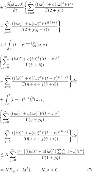
Theorem 4. Under Assumptions (24) and (25), Eq. (1) has a solution (x; t), which is asymptotically stable.
Proof. Consider a fractional elastic beam equation in the form of Eq. (1). Assume that j ~j < , j ~j < and j ~j < . Let (x; t) and (x; t) be, respectively, the solution of Eq. (1) and the following fractional elastic beam equation:
Dt~ + D~
x + aDx~ + b + n= 0: (77)
As a direct consequence of Eqs. (32) and (43), we obtain:
j(!; t) (!; t)j
=^0(!; 0)
(1 X
j=0
((i!)+ a(i!))jtj ~
(1 + j~)
1
X
j=0
((i!)+ a(i!))jtj(~+)
(1 + j(~ + )) )
+ t@ ^0(!; 0)@t (1
X
j=0
((i!)+ a(i!))jtj ~
(2 + j~)
1
X
j=0
((i!)+ a(i!))jtj(~+)
(2 + j(~ + )) )
+ b Z t
0 (t ) 1^
0(!; )
(1 X
j=0
((i!)+ a(i!))j(t )j ~
(~ + j~)
1
X
j=0
((i!)+ a(i!))j(t )j(~+)
(~ + + j(~ + )) )
d
+ Z t
0 (t ) 1^2
0(!; )
(1 X
j=0
((i!)+ a(i!))j(t )j ~
(~ + j~)
1
X
j=0
((i!)+ a(i!))j(t )j(~+)
(~ + + j(~ + )) )
d KX1
j=0
tj ~ ((i!)+ a(i!))P1
i=0( 1)iti
(1 + j~)
= KE;1~ ( t~); K; > 0: (78)
Therefore, by our assumption on , and , by means of the Fourier transform pair in Eq. (76), we nd that the solution is asymptotically stable.
7. Results and discussion
In this section, we apply the method presented in Section 3 to solve the following two test examples. The observations are depicted through Figures 1 and 2. Fig-ures 1 and 2 show the comparison between the obtained solutions in [25] and our approximate solutions for the nonlinear fractional beam equation, i.e. for:
D1
t(x; t) + Dx1(x; t) + a1Dx1(x; t) + b1
+ 2(x; t) = 0; (79)
(x; 0) = e0:1136x+ 0:5 + 0:0625e1 0:1136x; (80)
@(x; 0) @t =
0:8e0:1136x 0:0625 0:8 0:1136x
(e0:1136x+ 0:5 + 0:0625e 0:1136x2; (81)
and the following equation that can be achieved from
Figure 1. Approximate solution of Eq. (79) where x; t 2 [ 10; 10], 1= 2, 1= 4, 1= 2, a1= 2 and b1= 0:66.
Figure 2. Approximate solution of Eq. (82) where x 2 [0; 1], = 1, a2= 9 and b2= 4.
Eq. (1) using a travelling wave transformation: D4
x(x) + a2D2x(x) + b2(x) + 3(x) = 0; (82)
(0) = (1) = 2:735; 0(0) = 0:465;
0(1) = 0:465: (83)
We can obtain (x; t), as follows:
(x; t) =X1
k=0
k(x; t); (84)
where, in the rst example:
0(x; t) =
Z 1
1G1(x y; t)(y; 0)dy
+ Z 1
1G2(x y; t)
@(y; 0)
@t dy; (85) and:
k(x; t)
= b1 1
Z
1 t
Z
0
(t )1 1G
3(x y; t )k 1(y; )ddy
1
Z
1 t
Z
0
(t )1 1G
3(x y; t )k 12 (y; )ddy;
k = 1; 2; ; (86) where G1(x; t), G2(x; t) and G3(x; t) are dened by
Eqs. (37), (38) and (46), and in the second example:
0(x)=c0+c1x
!+c2E( pa
2x)+c3E( pa2x);
(87) where ci, i = 0; 1; 2; 3 can be determined by boundary
conditions and: k(x) = b2
Z 1
1G3(x y)k 1(y)dy
Z 1
1G3(x y) 3
k 1(y)dy;
k = 1; 2; ; (88) where:
G3(x) = 21
Z 1
1
1
(i!)4+ a2(i!)2e i!xd!: (89)
It is clear that the obtained results aided by Mathemat-ica 7.0 software are in close agreement with those ob-tained in [25]. Also, the method required to solve these problems uses only two iterations, while, in [25], the exp-function method required to solve the mentioned problems for an integer order of derivatives requires many manipulations. Therefore, for this case study, our proposed scheme obtained results having greater precision, a wider range, and require less iteration than the exp-function method.
8. Conclusions
In this manuscript, the homotopy perturbation method, with the help of joint Fourier-Laplace trans-forms, has been successfully applied to compute an analytical solution of a nonlinear fractional beam equa-tion. The convergence and stability of the homotopy perturbation method solution, as applied to this equa-tion, have been thoroughly investigated. The obtained results show that our approach provides the solution, in terms of the convergent series, with easily computable components in a direct way, and is very eective and
convenient for dealing with nonlinear fractional beam equations. Finally, the scheme can be applied to many physical problems, e.g., irregular signals, fractional Brownian motion and scale relativity.
References
1. Baleanu, D., Diethelm, K., Scalas, E. and Trujillo, J.J., Fractional Calculus Models and Numerical Methods, World Scientic (2012).
2. He, J.H. \Some applications of nonlinear fractional dierential equations and their applications", Bull. Sci. Technol., 15(2), pp. 86-90 (1999).
3. Agrawal, O.P. \A general solution for a fourth-order fractional diusion-wave equation dened in a bounded domain", Comput. Struct., 79, pp. 1497-1501 (2001).
4. He, J.H. \Homotopy perturbation technique", Com-put. Methdos Appl. Mech. Engrg., 178, pp. 257-262 (1999).
5. Odibat, Z. and Momani, S. \Modied homotopy per-turbation method: Application to quadratic Riccati dierential equation of fractional order", Chaos, Soli-tons Fractals, 36, pp. 167-174 (2008).
6. Dehghan, M. \A new operational matrix for solving fractional-order dierential equations", Comput. Math. Appl., 59, pp. 1326-1336 (2010).
7. Kumar, S. \A new analytical modelling for telegraph equation via Laplace transform", Appl. Math. Modell., 38(13), pp. 3154-3163 (2014).
8. Kumar, S. \A numerical study for solution of time frac-tional nonlinear Shallow-water equation in oceans", Zeits. Naturfor. A, 68a, pp. 1-7 (2013).
9. Kumar, S. \Numerical computation of time-fractional Fokker-Planck equation arising in solid state physics and circuit theory", Zeits. Naturfor., 68a, pp. 1-8 (2013).
10. Kumar, S. and Rashidi, M.M. \New analytical method for gas dynamics equation arising in shock fronts", Comput. Phys. Commun., 185(7), pp. 1947-1954 (2014).
11. He, J.H. \Homotopy perturbation method: a new nonlinear analytical technique", Appl. Math. Comput., 135, pp. 73-79 (2003).
12. He, J.H. \A tutorial review on fractal spacetime and fractional calculus", International Journal of Theor. Phys., 53(11), pp. 3698-3718 (2014).
13. Jafari, H. and Momani, S. \Solving fractional diusion and wave equations by modied homotopy perturba-tion method", Phys. Lett. A, 370, pp. 388-396 (2007).
14. Dehghan, M. and Shakeri, F. \The numerical solution of the second Painleve equation", Numer. Meth. Part. D.E., 25(5), pp. 1238-1259 (2009).
15. Golmankhaneh, A.R.K., Golmankhaneh, A.K. and Baleanu, D. \Homotopy perturbation method for
solv-ing a system of Schordesolv-inger-KdV equation", Rom. Journ. Phys., 63(3), pp. 609-623 (2011).
16. Gepreel, K.A. and Omran, S. \The exact solutions for the nonlinear partial fractional dierential equations", Chinese Phys., 21, pp. 110204-110211 (2012).
17. Herzallah, M.A.E. and Gepreel, K.A. \Approximate solution to the time-space fractional cubic nonlinear Schrodinger equation", Appl. Math. Modell., 36(11), pp. 5678-5685 (2012).
18. Gepreel, K.A. \The homotopy perturbation method to the nonlinear fractional Kolmogorov-Petrovskii-Piskunov equations", Appl. Math. Lett., 24, pp. 1428-1434 (2011).
19. Sayevand, K. \Ecient solution of fractional ini-tial value problems using expanding perturbation ap-proach", J. Math. Comput. Sci., 8(4), pp. 359-366 (2014).
20. Rektorys, K., Handbook of Applied Mathematics, 1(11), SNTL, Prague (1988).
21. Yu, R. and Zhang, H. \New function of Mittag-Leer type and its application in the fractional diusion-wave equation", Chaos Solit. Fract., 30, pp. 946-955 (2006).
22. Podlubny, I., Fractional Dierential Equations, San Diego, Academic Press (1999).
23. He, J.H., Elagan, S.K. and Li, Z.B. \Geometrical explanation of the fractional complex transform and
derivative chain rule for fractional calculus", Phys. Lett. A, 376(4), pp. 257-259 (2012).
24. He, J.H. \String theory in a scale dependent discontin-uous space-time", Chaos Solit. Fract., 36(3), pp. 542-545 (2008).
25. Zahra, K.A.A. and Hussain, M.A.A. \Exp-function method for solving nonlinear beam equation", Int. Math. Forum., 6, pp. 2349-2359 (2011).
Biographies
Khosro Sayevand received his BS degree from the University of Mazandaran, Iran, in 1997, his MS degree from Amirkabir University of Technology, Tehran, Iran, in 2000, and his PhD degree from Iran University of Science and Technology, Iran, in 2010, all in Applied Mathematics. He is currently Associate Professor at Malayer University, Iran. His current research interest mainly covers fractional calculus and numerical analysis. He has published more than 40 articles in these areas in ISI-listed journals.
Kazem Pichaghchi received BS and MS degrees in Mathematics from Semnan University, Iran, and Azarbaijan University of Tarbiat Moallem, Iran, in 2009 and 2011, respectively. His research interests include numerical analysis. At present he is a PhD degree student at Malayer University, Iran.