Sharif University of Technology
Scientia IranicaTransactions E: Industrial Engineering www.scientiairanica.com
A bi-objective mathematical model for dynamic cell
formation problem considering learning eect, human
issues, and worker assignment
M. Rabbani
, H. Habibnejad-Ledari, H. Raei and A. Farshbaf-Geranmayeh
School of Industrial Engineering, College of Engineering, University of Tehran, Tehran, Iran.Received 3 March 2015; received in revised form 14 August 2015; accepted 21 October 2015
KEYWORDS Dynamic cell formation; Human issues; Linear programming; Genetic algorithm; Central composite design.
Abstract. One of the important aspects neglected in the literature related to cell formation problem is human issues. In this study, a bi-objective mathematical model is developed in which human issues and dynamic cell formation are taken into consideration simultaneously. The rst objective function deals with costs associated with machines and human issues. The costs of human issues relate to salary, hiring, ring, reward/penalty policy, and worker assignment. The second objective function takes into account labor utilization as a criterion for reward/penalty policy. Since the available time in dierent real conditions is not constant, we include learning eect to consider the real workers time. The nature of dynamic cell formation problem is NP-hard, and thus a Linear Programming embedded Genetic Algorithm (LP-GA) is employed to solve the model. In order to improve the performance of the applied GA, its parameters are tuned by means of Central Composite Design (CCD) method. Moreover, to validate the LP-GA, some test problems are solved and the results are compared with those obtained from an exact method and GA. The computational results show that the near optimal solutions yielded by LP-GA are better than GA in large-sized problems.
© 2016 Sharif University of Technology. All rights reserved.
1. Introduction
Group Technology (GT) is a manufacturing approach that has positive impacts on batch-type production. Cellular Manufacturing System (CMS) is one of the aspects of GT which corresponds to the layout of manufacturing rms that can be used to enhance both exibility and eciency of the manufacturing system in today's global competitive environment. Aryanezhad et al. [1] and Raei and Ghodsi [2] stated that the
*. Corresponding author. Tel.: +98 21 88021067; Fax: +98 21 88350642
E-mail addresses: [email protected] (M. Rabbani); h [email protected] (H. Habibnejad-Ledari); [email protected] (H. Raei); [email protected] (A. Farshbaf-Geranmayeh)
most outstanding benets of CMS can be summarized as the reduction in lead time, setup time, and lot size. Also, Work-In-Process (WIP) and nished goods inventories as well as the throughput times are reduced, and working exibility are improved. Designing a CMS consists of the following steps: rst, part families are formed according to their processing requirements or geometric design; second, the machines are grouped into manufacturing cells; and third, part families are assigned to the cells [3]. The design of CMSs is called Cell Formation (CF). CF is a part of the CMS that attempts to group machines and part families into specied manufacturing cells. CF is one of the rst and most important steps in designing CMSs. Owing to high production variety, short product life cycle, volatile demand, and short delivery time, CMSs are
performed under dynamic environments [4]. In order to reach an optimal solution under this condition, changes, such as machine modication, should be taken into account.
Human issues should be considered in cellular manufacturing, because failing to take into account this factor can signicantly reduce the benets of cell manufacturing [4]. Bidanda et al. [5] stated that important human issues include worker assignment strategies, training, skill identication, reward/penalty system, communication, worker roles, teamwork, and conict management. This study presents a bi-objective model for the CF problem which considers learning eect, human issues, and some aspects of motivation in the rst objective function. The costs related to human issue consist of salary cost, hiring cost, ring cost, and worker assignment cost. Aspects of motivation such as reward/penalty policy are also taken into consideration. In addition, relevant costs of Dynamic Cell Formation Problem (DCFP) such as operational cost, inventory cost, and outsourcing cost are taken into account concurrently. Second objective function attempted to maximize the labor utilization. The problem being NP-hard, a Linear Programming embedded Genetic Algorithm (LP-GA) is employed, and its parameters are tuned by means of CCD method to solve the model. Also, the obtained results are compared with other approaches.
The remainder of the paper is organized as fol-lows. Section 2 presents the related literature review. Sections 3 and 4 present the model in details. In Section 5, the solution based on the methodology adopted is explained. In Section 6, some numerical examples are given to validate the model. Finally, the conclusion and directions for future research are presented in Section 7.
2. Literature review
Nowadays, manufacturing systems have become very important to the global business. A number of factors such as dynamic cell reconguration, sequence of op-erations, alternate part routings, operation time and cost, cost subcontracting, etc. are typically considered in manufacturing CF [6]. Paydar et al. [7] investigated CF and supply chain simultaneously. They presented a mixed integer linear programming and used a robust optimisation model to solve the proposed model. Jabal-Ameli and Moshref-Javadi [8] proposed a mathematical model for CF and layout design problems while consid-ering factors such as intra-cell and inter-cell layouts, part demands, operations sequence, etc. Saeidi et al. [9] developed a multi-objective mathematical pro-gramming model while considering production volume, machine redundancy, processing time, and sequence of operations to design a CMS and used a GA to solve
the proposed model. Bootaki et al. [10] presented a bi-objective model for cube CF. The rst part of the model sought to minimize the inter-cell movements, and the second part attempted to maximize a part quality index. Paydar and Saidi-Mehrabad [11] pre-sented a linear programming model in an attempt to maximize the grouping ecacy and developed a hybrid GA and Variable Neighborhood Search (VNS) to validate the model. Solimanpur et al. [12] took into account a number of intercellular movements and the number of voids simultaneously in a CF problem. Lian et al. [13] proposed a bi-objective model to minimize workload imbalance among manufacturing cells and applied a GA to solve it.
Rezazadeh et al. [14] proposed a new model that attempted to determine the optimal number of virtual cells and minimize the dierent costs such as produc-tion, material handling, subcontracting, etc. Kashan et al. [15] studied manufacturing CF problem that deals with grouping parts into families and machines into cells, with the aim of maximizing grouping ecacy. Saxena and Jain [16] dealt with Dynamic CF Prob-lem (DCFP) and presented a mixed integer nonlinear programming with the objective of minimizing costs as-sociated with machine operation, machine breakdown, production planning-related, etc. Bajestani et al. [17] proposed a multi-objective DCFP in an attempt to minimize the total cell load variation and the sum of the miscellaneous costs simultaneously. Shiyas and Pillai [18] developed an algorithm for the design of manufacturing cells and part families with the aim of maximizing grouping ecacy. Wang et al. [19] considered DCFP with three conicting objectives: the utilization rate of machine capacity, the total number of inter cell moves, and the machine relocation costs.
There are few studies on human issues in cellular manufacturing for several reasons, such as the diculty in the quantication of these issues. Failing to take into account human aspect of cellular manufacturing can considerably decrease the benets of this mode. Quantitative studies have demonstrated that labor-related issues have a critical impact on attaining optimal system performance in a CM [5]. Aryanezhad et al. [1] considered worker assignment and DCF simultaneously. They addressed machine exibility, part routing, and multi skill workers along with human cost issues related to hiring, ring, training, and salary. Raei et al. [4] presented a mathematical model that considered DCFP and worker assignment problem simultaneously as well as motivation, learning eect, and reward. They also incorporated machine-based and human-machine-based costs in their model. Norman et al. [20] presented a model involving human skills, training, worker assignment, and output quality with the objective of maximizing organization eectiveness.
Ghotboddini et al. [21] studied dynamic CMS and presented a model considering lean production. They attempted to minimize the reassignment cost of human resource, overtime cost of equipment, and labors; attempt was also made to maximize utilization rate of human resource. Raei and Ghodsi [2] investigated DCFP by a bi-objective mathematical formulation and attempted to minimize machine-based costs and also maximize labor utilization. They developed a hybrid ant colony optimization-GA approach to solve the model.
A list of the important features in CFP is given in Table 1. Also, Table 2 provides a summary of the researches reported on CFP in the literature.
In comparison with Aryanezhad et al. [1], Raei and Ghodsi [2], and Raei et al. [4], we dened a policy
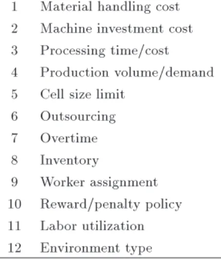
Table 1. List of important features in CFP. 1 Material handling cost
2 Machine investment cost 3 Processing time/cost 4 Production volume/demand 5 Cell size limit
6 Outsourcing 7 Overtime 8 Inventory
9 Worker assignment 10 Reward/penalty policy 11 Labor utilization 12 Environment type
for reward and penalty costs based on labor utilization and considered labor utilization levels for reward and penalty costs into the proposed model. However, a policy for reward and penalty was not considered in those two papers, and Raei et al. [4] took into account reward cost only as a part of objective function. Also, some relevant costs of DCFP, such as inventory and outsourcing, were taken into account in our proposed model, and we addressed labor utilization as the second objective function. Compared to Paydar et al. [7], Saxena and Jain [16], Defersha and Chen [22], and Arikan and Gungor [27], we considered human issues, namely, worker assignment, reward/penalty policy, and labor utilization. Also, we considered outsourcing, overtime, and inventory costs simultaneously.
3. Proposed model
In this section, a bi-objective mathematical model is presented in which the rst objective is to min-imize the costs of DCFP associated with machine procurement, inter-cell movement, machine relocation, machine variable, overtime, inventory, outsourcing, as well as human-related costs including ring, hiring, salary, reward/penalty policy, and worker assignment costs. The second objective function aims to maximize labor utilization. In this model, a CMS is conceived to comprise a number of machines for processing dierent parts. Learning curve is considered in the model to improve benets and organizational productivity in reward systems [4]. Newly hired labors are less ecient than the experienced ones, but they can improve their productivity by repeating their tasks [28,29].
Table 2. Overview of the literature on CFP.
Paper Feature
1 2 3 4 5 6 7 8 9 10 11 12
Aryanezhad et al. [1] x x x x x x 1
Raei and Ghodsi [2] x x x x x x x 1
Raei et al. [4] x x x x x x 1
Paydar et al. [7] x x x x x x 2
Saeidi et al. [9] x x x x 2
Saxena and Jain [16] x x x x x x x 1
Wang et al. [19] x x x x 1
Defersha and Chen [22] x x x x x x x 1
Cao et al. [23] x x x x 1
Egilmez et al. [24] x x 2
Sudhakara Pandian and Mahapatra [25] x 1
Chung et al. [26] x x x x 1
Arikan and Gungor [27] x x x x x x 2
This paper x x x x x x x x x x x 1
According to the learning curve, the time of an action will be equal to t0ib after some iterations, where t0 is
the initial time of the job activity, i is the number of iterations, and b is a negative coecient [25,26]. 3.1. Mathematical model
Assumptions
Demand for each part type, time capacity of each machine type, and processing time for all operations of a part type in each period are known and deterministic;
All machines of type m can process all part types, p;
Each machine type m can perform one or more operations, called machine exibility;
Each operation can be performed on one or more machine types with dierent times, called routing exibility [1];
The machines purchasing costs are known and they are purchased with a certain limit;
Machines are grouped into relatively independent cells with minimum inter-cell movement of the parts;
Parts are moved between cells in batches (regardless of the distance traveled);
The maximum number of used cells, bounds, and quantity of machines in each cell need to be specied in advance, and maximum number of cells remains constant over time;
Each machine needs just one labor;
Relocation cost of each machine between periods is known;
In order to process a certain operation, the related machine and labor must be available at the same time [1];
Backorders are not allowed;
Workload of the cells should be balanced [16];
Inventory is equal to zero in the beginning and at the end of the planning horizon;
Learning curve is considered in the model to increase the benets and organizational productivity of the systems.
Indices
c Manufacturing cell (c = 1; ; C); m Machine type (m = 1; ; M); p Part type (p = 1; ; P ); t Time period (t = 1; ; T ); j Operations belonging to part
p (j = 1; ; Op);
t0 Time period labors hired (t0 =
1; ; T ).
Parameters
C Number of cells; M Number of machines; P Number of part types; T Number of periods;
Op Number of operations for part type p;
Dpt Demand for part type p in time period
t; Binter
p Batch size for inter-cell movements of
part type p; inter
p Inter-cell movement cost per batch of
part type p;
m Purchase cost of machine type m; m Marginal revenue from selling machine
type m;
m Fixed cost of machine type m in each
time period;
Cm Variable cost of machine type m for
each unit time in regular time intervals; mt Variable cost of processing on machine
type m per hour in overtime in time period t;
+
m Relocation cost of installing one
machine of type m;
m Relocation cost of removing one machine of type m;
ICpt Inventory cost of per part type p in
time period t;
OCpt Outsourcing cost of part type p in time
period t;
Sct Salary cost of each labor in cell c in
time period t;
hct Hiring cost of each labor used in cell c
in time period t;
fct Firing cost of each labor red from cell
c in time period t; r
ct Reward cost for labors in cell c in time
period t;
pct The value earned from each labor penalty in cell c in time period t; Tmt Time capacity of machine type m in
time period t at regular time intervals; T0
mt Time capacity of machine type m in
time period t in overtime;
A Available working time for each worker in hours per time period;
LB Lower bound of the cell size; UB Upper bound of the cell size; tjpm Processing time required to perform
operation j of part type p on machine type m;
t0
jpm Manual workload time required to
perform operation j of part type p on machine type m;
b Learning index;
q Balancing factor of inter-cell workload, (0 q 1);
R A big number;
AW Level of labor utilization which deserves reward;
P U Level of labor utilization which deserves penalty.
Decision variables
Nmct Number of machines type m allocated
to cell c in time period t;
Xjpmct Number of parts type p processed by
operation j on machine type m in cell c in time period t;
I+
mt Number of machines type m purchased
in period t;
Imt Number of machines type m sold in period t;
K+
mct Number of machines type m added in
cell c in period t;
Kmct Number of machines type m removed in cell c in period t;
Xpt Number of parts type p processed in
period t;
Qpt Number of part inventory of type p
kept in period t and carried over to period t + 1;
Opt Number of parts type p to be
subcontracted in period t;
Wct0t Number of labors assigned for cell c in
period t hired in period t0;
Wct Number of labors assigned for cell c in
period t;
Hct Number of labors hired for cell c in
period t;
Fct Number of labors red for cell c in
period t;
LUct Labor utilization in cell c in period t;
Zjpct 1, if operation j of type p is done in
cell c in period t; 0 otherwise;
#pt 1, if part p is set up for production in
period t; 0 otherwise; T0
mct Amount of extra time required by
machine m located in cell c in period t; yr
ct 1, if LUct is more than AW ; 0
otherwise;
yctp 1, if LUct is less than P U; 0 otherwise.
Objective function
min z1= T P t=1 C P c=1 M P
m=1Nmctm
(1) +PT
t=1 C P c=1 M P m=1 P P p=1 Op P
j=1CmXjpmcttjpm
(2) +PT
t=1 M
P
m=1I + mtm
T
P
t=1 M
P
m=1Imt m
(3) (4) +PT
t=1 C P c=1 M P m=1 + mKmct+
(5) +PT
t=1 C P c=1 M P
m=1mKmct
(6) +1 2 T P t=1 C P c=1 P P p=1 OPp 1
j=1 inter
p Binter
p
:Xpt Z(j+1)pct Zjpct
(7) +PT
t=1 P
P
p=1ICptQpt+ T
P
t=1 P
P
p=1OCptOpt
(8) (9) +PT
t=1 C P c=1 M P m=1T 0 mctmt
(10) +PT
t=1 C P c=1 T P
t0=1
SctWct0t
(11) +PT
t=1 C
P
c=1hctHct+ T
P
t=1 C
P
c=1fctFct
(12) (13) +PT
t=1 C P c=1 T P
t0=1
r
ctWct0tyctr
(14) T P t=1 C P c=1 T P
t0=1
p
ctWct0tyctp
max z2= T
P
t=1 C
P
c=1LUct
(16) Subject to:
C
X
c=1
Zjpct= #pt 8j; p; t; (17)
Xjpmct R:#pt 8j; p; m; c; t; (18)
P
X
p=1 Op
X
j=1
XjpmcttjpmZjpct TmtNmct+ Tmct0
8m; c; t; (19)
C
X
c=1
T0
mct Tmt0 8m; t; (20)
wct= wc(t 1)+ Hct Fct 8c; t; (21)
where:
wct= T
X
t0=1
Wct0t 8c; t;
A
C
X
c=1
(t t0)bWct0t+ Hct Fct
XC
c=1 M
X
m=1
TmtNmct+ C
X
c=1 M
X
m=1
T0 mct
8t; t0< t; (22) C
X
c=1
Nmct C
X
c=1
Nmc(t 1)= Imt+ Imt 8m; t; (23)
Nmc(t 1)+ Kmct+ Kmct= Nmct; 8m; c; t; (24) M
X
m=1
Nmct LB 8c; t; (25)
M
X
m=1
Nmct UB 8c; t; (26)
Qp(t 1)+ Opt+ Xpt Qpt Dpt 8p; t; (27)
where:
Xpt= C
X
c=1 M
X
m=1
Xjpmct 8j; p; t;
M
X
m=1 P
X
p=1 Op
X
j=1
XjpmcttjpmZjpct
q 2 4 1
C
C
X
c=1 M
X
m=1 P
X
p=1 Op
X
j=1
XjpmcttjpmZjpct
3 5
8c; t; (28)
PM
m=1
PP
p=1
POp
j=1Xjpmctt0jpmZjpct
WctA LUct
8c; t; (29)
LUct AW Ryctr 8c; t; (30)
LUct P U R(1 ypct) 8c; t; (31)
Zjpmct;yctr; ypct; #pt; amct2 f0; 1g; LUct
2 [0; 1]; Xjpmct; Xpt; Qpt; Opt; Tmct0 0;
8j; p; m; c; t; (32) Nmct;Imt+ ; Imt; Kmct+ ; Kmct; Wct0t; Wct; Hct; Fct
0 and integer 8m; c; t; t0: (33)
The rst objective function consists of dierent cost terms as follows: Term (1) represents xed cost of machines and depends on the number of machines. Term (2) indicates machine variable cost. Term (3) shows machine procurement cost. Term (4) denotes machine selling income. Terms (5) and (6) represent machine relocation cost which consists of installing and removing costs. Term (7) shows inter-cell movement cost. Term (8) represents part holding cost. Term (9) indicates part outsourcing cost. Term (10) represents overtime cost. Terms (11)-(13) show labors salary, hiring, and ring costs. Terms (14) and (15) refer to reward and penalty costs. Lastly, labor utilization is maximized by the second objective function (i.e., Term (16)).
Eq. (17) and Constraint (18) guarantee that parts are processed if they are planned to produce. Constraint (19) ensure time capacities of planning periods. Constraint (20) limit the utilized extra time. Eq. (21) represent the labor balancing equation. Constraint (22) satisfy the total demand in each period. Eqs. (23) and (24) balance machine quantities between any successive planning periods. Constraints (25) and (26) ensure lower and upper bounds of the number
of machines in cells. Constraint (27) show that demand of part type p in each time period t is satised through internal part production, part outsourcing, and/or part inventory carried over from the previous period t 1. Constraint (28) enforce workload balance among cells. Labor utilization is modeled by inequality Constraint (29). Constraints (30) and (31) indicate the applied reward or penalty policy, which depends on labor utilization value. Finally, types and ranges of all variables are presented in Constraints (32) and (33). The model is then converted into a single objec-tive model using the Weighted Sum Method (WSM). Term (16) is incorporated into the rst objective function with a negative coecient as follows:
T
X
t=1 C
X
c=1
LUct: (34)
In order to prevent scaling problem, normalization of the objective functions should be taken into account. It is assumed that F1 refers to the rst objective
function and F2 is the second objective function. yI1
and yI
2 are ideal solutions of the rst and second
objective functions, respectively. yN
1 and y2N are nadir
solutions of the rst and second objective functions, respectively. Also, W1 and W2 are weights of the
rst and second objective functions, respectively. The integrated objective function is given as follows:
F = W1 F1 y I 1
yN
1 y1I + W2
F2 yI2
yI
2 yN2 : (35)
3.2. Model simplication
The presented model is nonlinear due to the 7th, 14th, and 15th terms of the objective function, the time capacity constraints (Eq. (19)), the workload balancing constraints (Eq. (28)), and labor utilization constraints (Eq. (29)). The nonlinear term XptjZ(j+1)pct Zjpctj
in the 7th term can be linearized by Eqs. (36)-(40) and is then replaced by variable jpmct. The nonlinear
term Wct0t:yctr in the 14th term and Wct0t:yctp in the
15th term can be linearized through Eqs. (41)-(43) and (44)-(46) and are replaced by variables Ect0t and
EEct0t, respectively. The nonlinear term Xjpmct:Zjpct
in Eqs. (19), (28), and (29) are linearized by Eqs. (47)-(49) and is replaced by the variable Gjpmct.
Z(j 1)pct Zjpct jpct 8j; p; c; t; (36)
Z(j 1)pct+ Zjpct jpct 8j; p; c; t; (37)
jpmct Xjpmct 8j; p; m; c; t; (38)
jpmct R:jpct 8j; p; m; c; t; (39)
jpmctXjpmct R(1 jpct) 8j; p; m; c; t; (40)
Ect0t Wct0t 8c; t0; t; (41)
Ect0t R:yrct 8c; t0; t; (42)
Ect0t Wct0t R(1 yrct) 8c; t0; t; (43)
EEct0t Wct0t 8c; t0; t (44)
EEct0t R:ypct 8c; t0; t; (45)
EEct0t Wct0t R(1 yctp) 8c; t0; t; (46)
Gjpmct Xjpmct 8j; p; m; c; t; (47)
Gjpmct R:Zjpct 8j; p; m; c; t; (48)
GjpmctXjpmct R(1 Zjpct) 8j; p; m; c; t; (49)
jpct2 f0; 1g; jpmct; Ect0t; EEct0t; Gjpmct 0
8j; p; m; c; t: (50)
4. Solution methodology
In this section, the hybrid LP-GA approach as the applied methodology is discussed in detail.
4.1. LP-GA approach
Due to the NP-hard nature of the problem, a LP-GA approach is applied to solve it. LP-GA is one of the optimization approaches based on the mechanism of natural selection. This algorithm attempts to mimic natural processes in order to create optimization proce-dures. GA has gained increasing popularity for solving dierent optimization problems and has been used in dierent areas such as engineering, manufacturing, etc. [30]. A GA starts with a feasible solution and in each iteration, the current solution is replaced with a new one [31]. To reproduce and generate osprings, GA uses genetic operators which generally consist of selection, crossover, and mutation. Also, GA utilizes a tness function to measure the quality of each encoded solution. Some of the typical unique features of GA that distinguish it from other algorithms include population-based search, searching and evaluating a large number of feasible points in the solution space, implicit parallelism, exibility of hybridizing with other domain-dependent heuristics, and taking advantage of the probabilistic theory for selection to direct their search [30]. Based on the foregoing discussion, GA can decrease the possibility of being trapped in a local optima. In the developed algorithm, the values of the integer variables are obtained by decoding the solution representation. Also, using an optimization software, a linear programming is solved to nd the corresponding values of the continuous variables and
those of the objective function. The advantage of LP-GA approach is that when the LP is solved, values that optimally correspond to the integer solution can be yielded simply. Also, while it appears to be hard to satisfy several constraints with continuous variables through only GA, the LP satises them easily [22]. 4.2. Chromosome representation
The rst step in GA is designing chromosome charac-teristics to devise a suitable representation scheme and maintaining the feasibility of the generated chromo-somes. Each chromosome is represented by a sequence of genes which can be a set of real, binary or integer numbers, symbols, and matrices. Two approaches are used to represent the chromosome: direct and indirect encodings. In a direct encoding, a chromosome totally represents a solution, while in an indirect encoding, a chromosome involves data which are used to achieve a solution [31]. In this paper, both direct and indirect coding schemes are used to represent the chromosomes. In the proposed representation, four types of chromo-somes (i.e., N, W , #, and L) are considered. The rst two chromosomes which are related to decision variables, Nmct and Wct0t, are m c t and c t0 t
matrices, respectively. The last two chromosomes which relate to decision variables, #ptand Ljp, are pt
and j p matrices, respectively. The chromosome N which denotes the number of machines type m installed in cell c during time period t takes a positive integer value. The second chromosome is W which takes a positive integer value. It indicates the number of labors assigned to cell c during time period t which is used in time period t0. The chromosome # is a binary variable
that shows whether or not part p has been planned for production in time period t. The chromosome L takes a value in f1; ; Cg and shows the index of the cell in which operation j of part type p is to be processed. 4.3. Decoding chromosomes
The values of decision variables Nmct, Wct0t, and #pt
are read directly from the chromosome, while the decision variable, Zjpct, is determined using Eq. (51).
Based on this equation, the constraint in Eq. (17) can be satised.
Zjpct=
(
#pt if the subscript c = Ljp
0 otherwise (51)
Also, decision variables K+
mct, Kmct, Imt+, Imt, Hct, and
Fct can be determined using Eqs. (52)-(57),
respec-tively. These equations satisfy Constraints (21)-(24).
K+ mct =
(
Nmct if t = 1
maxf0; Nmct Nmc(t 1)g if t > 1 (52)
Kmct = (
0 if t = 1
maxf0; Nmc(t 1) Nmctg if t > 1 (53)
I+ mt= 8 > > < > > : C P
c=1Nmct if t=1
max
0;PC
c=1Nmct C
P
c=1Nmc(t 1)
if t>1 (54)
Imt= 8 < :
0 if t=1
max
0;PC
c=1Nmc(t 1) C
P
c=1Nmct
if t>1 (55)
Hct=
8 > > > > > > > > > > < > > > > > > > > > > : T P
t0=1
Wct0t
if t = 1; t0 t
max
0; PT
t0=1
Wct0t T
P
t0=1
Wct0(t 1)
if t > 1; t0 t
(56)
Fct=
8 > > > > > > > > < > > > > > > > > : 0
if t = 1
max
0; PT
t0=1
Wct0(t 1) T
P
t0=1
Wct0t
if t > 1; t0 t
(57)
4.4. LP method
The values of all the integer decision variables are obtained by decoding a chromosome and using the penalty method as explained in the previous sections. The constraints containing only the integer variables are satised by decoding the chromosomes except Constraints (25) and (26), which are dealt with by the penalty method. The corresponding continuous values are determined by solving a linear programming. The objective function of this LP involves Terms (2), (7)-(10), and (34) subject to the constraints in Eqs. (18)-(20), (22), and (27)-(31). First, the integer variables are satised by proposed GA, and the model with the corresponding continuous values are solved by branch and bound algorithm using GAMS optimization software.
4.5. Fitness function
Fitness function is used to evaluate the candidate solutions in the population and reproduce new chro-mosomes, called osprings. In the proposed algorithm, the tness value of a chromosome is dened as the objective function value (Terms (1)-(15) and (34)) and the penalty term of constraints violation. The factor
PV is used to scale the penalty term.
Fitness function = model objective function
+ P V
T
X
t=1 C
X
c=1
max (
0; LB
M
X
m=1
Nmct; M
X
m=1
Nmct UB
)
: (58)
4.6. Selection
The Roulette Wheel selection procedure is a tness-proportional selection in which an individual with higher tness will be selected with a higher probabil-ity [32]. In this procedure, all individuals will have a chance to be selected, but superior individuals will have a higher selection probability.
4.7. Genetic operators
Crossover and mutation, as two genetic operators, are used to produce new osprings from the selected parents. The crossover and mutation used in the proposed model are discussed below.
4.7.1. Crossover
Crossover as the main genetic operator combines in-formation from two parents and reproduces two new chromosomes. In this paper, a uniform crossover is applied to produce new chromosomes. In the uniform crossover, the binary chromosome is randomly gener-ated as large as the main chromosome. For ospring 1, if = 1, the gene is taken from parent 1; if = 0, the gene is taken from parent 2. For ospring 2, if = 1, the gene is taken from parent 2; if = 0, the gene is taken from parent 1. Eq. (59) shows the proposed crossover:
Ospring 1 = parent 1 + (1 ) parent 2; Ospring 2= parent 2+(1 ) parent 1: (59) The pseudo code of the proposed crossover operator for variable Nmct is shown in Figure 1.
4.7.2. Mutation
Mutation operator is used to keep the diversity of the population at a reasonable level with producing random changes in a chromosome. In this paper, a
binary mutation is applied to produce new chromo-somes. In the binary mutation, rst, we determine parameter usually equal to 0.001 or 0.01. The number of mutations (nm) is then specied by means of the equation represented below (where N denotes the number of genes in the chromosome). Subsequently, genes are selected randomly and mutation operator is applied to the chromosome. Based on the chromosome type, the selected genes can take dierent values.
nm = [ N] + 1: (60) For example, a random value is generated between [1; C], and assigned to the selected gene in chromosome L for Ljp.
4.8. Parameters tuning
The performance of GA strongly relies on its param-eters including population size, number of iterations, crossover probabilities, and mutation probabilities. As a single set of GA, the parameters are not guaranteed to obtain a near-optimum solution for the problem. The Central Composite Design (CCD) method is applied to tune GA parameters so as to determine appropriate population size and number of iterations, as well as crossover and mutation probabilities. CCD, also called response surface methodology, extracts the relationship between responses and eective factors [33]. By imple-menting the CCD, regression coecients for eective factors are extracted. Then, an optimization software is applied to nd the optimum combination of eective factors. Factors and their levels are shown in Table 1.
5. Computational results
To demonstrate the performance of the proposed al-gorithm and to verify the feasibility of the proposed model, 25 numerical samples are tested. Tables 3 and 4 present data of the numerical examples. In Table 5, the range of parameters used in the model is presented. These parameters are generated uniformly. The LP-GA approach has been coded in Matlab 7 and run on a PC core i5, 1.8 GHz speed with 6 GB of RAM.
In these tests problems, lower and upper bounds are 2 and 6, respectively. Batch size is 40 and the cost of each batch is equal to 30. Dierent learning rates have been considered in the literature. Heizer and Render [34] showed that the learning rate could
Table 3. Designed factors and their levels.
Factors Levels
Low High Iteration (maxit) 150 250 Population size (npop) 100 200 Crossover probability (pc) 0.7 0.8 Mutation probability (pm) 0.3 0.4
Table 4. Test problems.
No. J P M C T
1 3 4 4 2 2
2 4 4 4 2 2
3 5 5 5 2 2
4 6 5 5 2 2
5 6 6 5 3 2
6 6 6 6 3 3
7 7 7 6 3 3
8 8 7 7 3 3
9 7 8 7 3 3
10 8 8 7 3 2
11 8 8 8 3 3
12 9 8 8 3 3
13 9 9 9 3 3
14 10 10 10 3 2
15 11 11 11 3 3
16 12 12 12 3 3
17 14 14 12 3 3
18 15 15 15 4 3
19 17 17 15 4 3
20 18 20 16 4 2
21 19 19 16 4 2
22 19 22 17 4 2
23 20 23 18 4 2
24 20 25 20 4 2
25 22 27 20 4 2
range between 0.7 and 0.9 for dierent industries. Also, several studies, such as [35,36], considered the learning rate to be at the interval of [0:7 0:9]. In this paper, this rate is assumed to be 0.85. It should be mentioned that the learning index (b) is calculated as the logarithm
Table 5. Data of the test problems. Parameter Data
range Parameter
Data range Dpt [200 300] t0jpm [5 8]
mt [20 35] m [550 680]
Sct [150 180] m [300 500]
hct [140 170] m [5 10]
fct [15 17] Cm [5 10]
Tmt [700 800] +m [30 40]
T0
mt [140 160] m [30 40]
tjpm [3 5]
to base 2 of learning rate (i.e., b = 0:2). The parameters of AW , P U, and q are determined with the coordination of three academic and two industrial experts. Based on their opinions, the value of AW , P U, and q are assumed to be 0.8, 0.4, and 0.5, respectively. The inventory cost is 150, outsourcing cost is 300, and the reward and penalty values are 40 and 30, respectively.
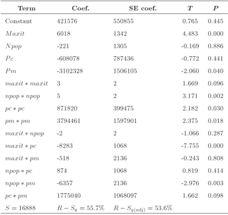
To improve the performance of the proposed approach, eective GA parameters are tuned by CCD. Each parameter takes values in dierent levels. So, to obtain reasonable computational results, a CCD method is adopted to determine the best levels of the parameters including maxit, npop, pc, and pm. More-over, regression coecients are extracted and shown in Table 6. Also, the optimum solutions obtained from GAMS are shown in Table 7. The values maxit = 150, npop = 200, pc = 0:7, and pm = 0:4 are selected to improve the performance of proposed algorithm.
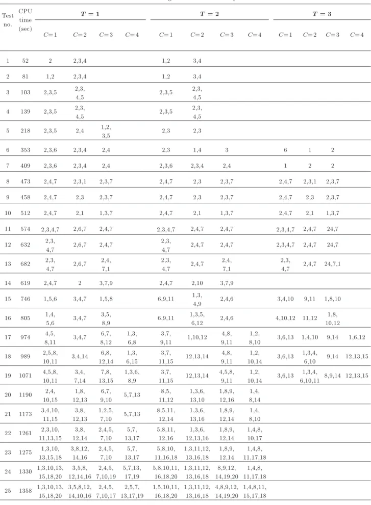
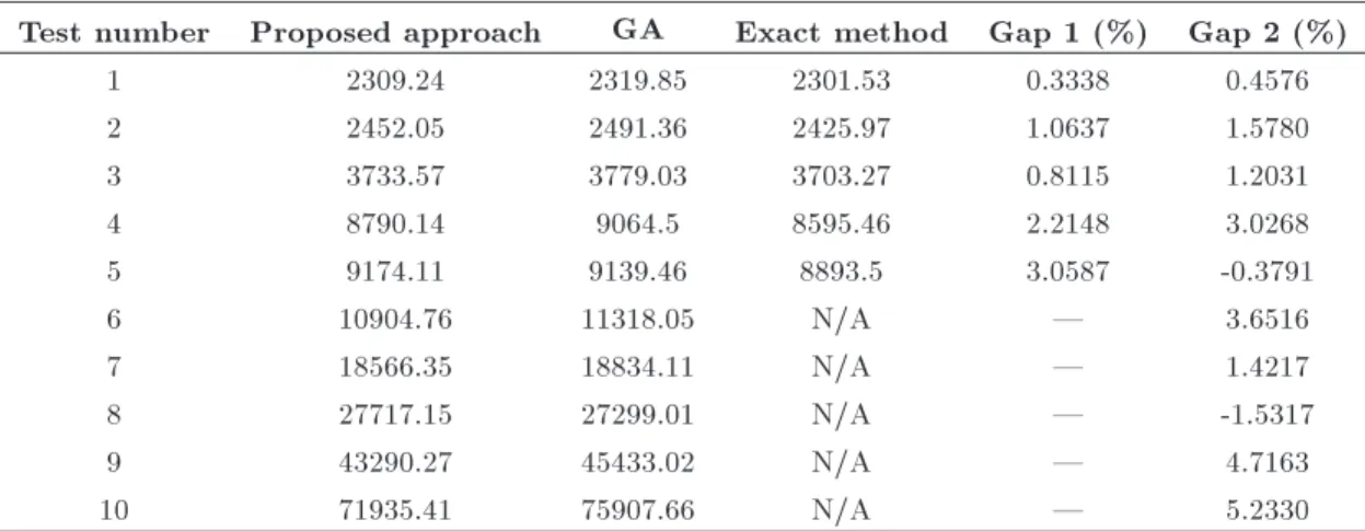
The obtained results of the problems are shown in Table 8. In this table, numbers in each cell correspond to the machines and demonstrate the ones that are assigned to the cells. Also, the CPU running time of algorithm is presented in Table 8. Table 9 shows the results of the 10 test problems applying two methods (GA and an exact method) and shows a comparison of these methods and our proposed GA-TS. In the exact method, the branch and bound algorithm is applied using GAMS optimization software. The following formula is used for computing the gaps:
Gap 1 =proposed approach exact methodproposed approach ; (61)
Gap 2 =GA proposed approach
GA : (62)
Table 9 shows the performance of proposed GA-TS algorithm with respect to the GA algorithm and the exact method. Each test problem is solved 15 times and we choose the minimum cost. Table 9 shows
Table 6. Estimated regression coecients.
Term Coef. SE coef. T P
Constant 421576 550855 0.765 0.445
Maxit 6018 1342 4.483 0.000
Npop -221 1305 -0.169 0.886
P c -608078 787436 -0.772 0.441
P m -3102328 1506105 -2.060 0.040
maxit maxit 3 2 1.669 0.096
npop npop 5 2 3.171 0.002
pc pc 871820 399475 2.182 0.030
pm pm 3794461 1597901 2.375 0.018
maxit npop -2 2 -1.066 0.287
maxit pc -8283 1068 -7.755 0.000
maxit pm -518 2136 -0.243 0.808
npop pc 874 1068 0.819 0.414
npop pm -6357 2136 -2.976 0.003
pc pm 1775040 1068097 1.662 0.098
S = 16888 R Sq= 55:7% R Sq(adj)= 53:6%
Table 7. Optimum values of GA factors obtained from CCD.
Maximum iteration
(maxit)
Population size (npop)
Crossover probability
(pc)
Mutation probability
(pm)
150 200 0.7 0.4
that the proposed approach has acceptable capacity to obtain a good solution in large-sized problems. Also, if the results of the proposed algorithm are compared with those of GA, the proposed algorithm obviously outperforms this algorithm. The values of Gaps 1 and 2 are presented in Table 9.
6. Conclusions and directions for future research
Human-related issues such as problems associated with salary, hiring, ring, and worker assignment are among the most important issues in DCFP, which have been ignored in the literature. In this paper, a new bi-objective mathematical model was proposed to deal with dynamic CF and human-related issues. The rst objective function was separated into two parts. The rst part was related to machine-based costs, such as operational cost, inter-cell movement cost, machine procurement cost, relocation cost, machine variable cost, inventory cost, outsourcing cost, and overtime
cost. The second part was related to human-related costs including salary, hiring, ring, and worker assign-ment costs. In this part, some aspects of motivation, namely reward/penalty policy, were also taken into account. The second objective function considered labor utilization which is a criterion for reward/penalty policy. Since, in the real world, the available time in dierent conditions is not constant, in order to indicate the real workers time, learning eect was incorporated in the model. The problem was NP-hard, and thus a LP-GA approach was employed to solve the model. Also, to improve the performance of the proposed approach, eective GA parameters were tuned by the CCD. Furthermore, to validate the proposed approach, several test problems with dierent sizes were generated randomly and solved by an exact method, GA, and the proposed approach. Lastly, the results obtained were compared with each other. Computational results show that the proposed approach enjoys the potential to obtain good solution in large-sized problems. Also, it outperforms the GA in most of the test problems.
In order to increase system exibility, cross-training is often used. It results in multi-skilled operators and reduces the processing time and the time periods that depend on operator. Considering cross-training can be a signicant contribution to continue the current research directions. Also, Our purpose was to investigate human issues theoretically, and their
Table 8. Cell congurations of the test problems. Test no. CPU time (sec)
T = 1 T = 2 T = 3
C=1 C=2 C=3 C=4 C=1 C=2 C=3 C=4 C=1 C=2 C=3 C=4
1 52 2 2,3,4 1,2 3,4
2 81 1,2 2,3,4 1,2 3,4
3 103 2,3,5 2,3,
4,5 2,3,5
2,3, 4,5
4 139 2,3,5 2,3,
4,5 2,3,5
2,3, 4,5
5 218 2,3,5 2,4 1,2,
3,5 2,3 2,3
6 353 2,3,6 2,3,4 2,4 2,3 1,4 3 6 1 2
7 409 2,3,6 2,3,4 2,4 2,3,6 2,3,4 2,4 1 2 2
8 473 2,4,7 2,3,1 2,3,7 2,4,7 2,3 2,3,7 2,4,7 2,3,1 2,3,7
9 458 2,4,7 2,3 2,3,7 2,4,7 2,3 2,3,7 2,4,7 2,3 2,3,7
10 512 2,4,7 2,1 1,3,7 2,4,7 2,1 1,3,7 2,4,7 2,1 1,3,7
11 574 2,3,4,7 2,6,7 2,4,7 2,3,4,7 2,4,7 2,4,7 2,3,4,7 2,4,7 24,7
12 632 2,3,
4,7 2,6,7 2,4,7
2,3,
4,7 2,4,7 2,4,7 2,3,4,7 2,4,7 24,7
13 682 2,3,
4,7 2,6,7 2,4, 7,1 2,3, 4,7 2,4,7 2,4, 7,1 2,3,
4,7 2,4,7 24,7,1
14 619 2,4,7 2 3,7,9 2,4,7 2,10 3,7,9
15 746 1,5,6 3,4,7 1,5,8 6,9,11 1,3,
4,9 2,4,6 3,4,10 9,11 1,8,10
16 805 1,4,
5,6 3,4,7 3,5,
8,9 6,9,11
1,3,5,
6,12 2,4,6 4,10,12 11,12
1,8, 10,12
17 974 4,5,
8,11 3,4,7 6,7, 8,12 1,3, 6,8 3,7, 9,11 1,10,12 4,8, 9,11 1,2,
8,10 3,6,13 1,4,10 9,14 1,6,12 18 989 2,5,8,
10,11 3,4,14 6,8, 12,14 1,3, 6,15 3,7, 11,15 12,13,14 4,8, 9,11 1,2, 10,14 3,6,13 1,3,4,
6,10 9,14 12,13,15 19 1071 4,5,8,
10,11 3,4, 7,14 7,8, 13,15 1,3,6, 8,9 3,7, 11,15 12,13,14 4,5,8, 9,11 1,2, 10,14 3,6,13 1,3,4,
6,10,11 8,9,14 12,13,15 20 1190 2,4,
10,15 1,8, 12,13 6,7, 9,10 5,7,13 8,5, 11,12 1,3,6, 13,10 1,8,9, 12,16 1,4, 8,14 21 1173 3,4,10,
11,15 3,8, 12,13 1,2,5, 7,10 5,7,13 8,5,11, 12,14 1,3,6, 13,16 1,8,9, 12,14 1,4, 8,10 22 1261 2,3,10,
11,13,15 3,8, 12,14 2,4,5, 7,10 5,7, 13,17 5,8,11, 12,16 1,3,6, 12,13,16 1,8,9, 12,14 1,4,8, 10,17 23 1275 1,3,10,
13,15,18 3,8,12, 14,16 2,4,5, 7,10 5,7, 13,17 5,8,10, 11,16,18 1,3,11,12, 13,16,18 1,8,9, 12,14 1,4,8, 11,17,18 24 1330 1,3,10,13,
15,18,20 3,5,8, 12,14,16 2,4,5, 7,10,19 5,7,13, 17,19 5,8,10,11, 16,18,20 1,3,11,12, 13,16,18 8,9,12, 14,19,20 1,4,8, 11,17,18 25 1358 1,3,10,13,
15,18,20 3,5,8,12, 14,10,16 2,4,5, 7,10,17 2,5,7, 13,17,19 1,5,10,11, 16,18,20 1,3,11,12, 13,16,18 4,8,9,12, 14,19,20 1,4,8,11, 15,17,18
Table 9. Performance of proposed method compared to other approaches.
Test number Proposed approach GA Exact method Gap 1 (%) Gap 2 (%)
1 2309.24 2319.85 2301.53 0.3338 0.4576
2 2452.05 2491.36 2425.97 1.0637 1.5780
3 3733.57 3779.03 3703.27 0.8115 1.2031
4 8790.14 9064.5 8595.46 2.2148 3.0268
5 9174.11 9139.46 8893.5 3.0587 -0.3791
6 10904.76 11318.05 N/A | 3.6516
7 18566.35 18834.11 N/A | 1.4217
8 27717.15 27299.01 N/A | -1.5317
9 43290.27 45433.02 N/A | 4.7163
10 71935.41 75907.66 N/A | 5.2330
applications could be considered as future research direction for interested researchers.
References
1. Aryanezhad, M.B., Deljoo, V. and Mirzapour Al-e-hashem, S.M.J. \Dynamic cell formation and the worker assignment problem: A new model", Int. J. Adv. Manuf. Tech., 41(3-4), pp. 329-342 (2009). 2. Raei, H. and Ghodsi, R. \A bi-objective
mathemat-ical model toward dynamic cell formation considering labor utilization", Appl. Math. Model., 37(4), pp. 2308-2316 (2013).
3. Papaioannou, G. and Wilson, J.M. \The evolution of cell formation problem methodologies based on recent studies (1997-2008): Review and directions for future research", Eur. J. Oper. Res., 206(3), pp. 509-521 (2010).
4. Raei, H., Rabbani, M. and Koushan, M. \Eect of motivation and learning curve in dynamic cell formation and the worker assignment problem", Int. J. Eng. Sci. Res. Tech., 1(9), pp. 481-497 (2012). 5. Bidanda, B., Ariyawongrat, P., Needy, K.L., Norman,
B.A. and Tharmmaphornphilas, W. \Human related issues in manufacturing cell design, implementation, and operation: A review and survey", Comput. Ind. Eng., 48(3), pp. 507-523 (2005).
6. Defersha, F.M. and Chen, M. \Machine cell formation using a mathematical model and a genetic algorithm-based heuristic", Int. J. Prod. Res., 44(12), pp. 2421-2444 (2006).
7. Paydar, M.M., Saidi-Mehrabad, M. and Teimoury, E. \A robust optimisation model for generalized cell formation problem considering machine layout and supplier selection", Int. J. Comput. Integr. Manuf., 27(8), pp. 772-786 (2014).
8. Jabal-Ameli, M.S. and Moshref-Javadi, M. \Concur-rent cell formation and layout design using scatter search", Int. J. Adv. Manuf. Tech., 71(1-4), pp. 1-22 (2014).
9. Saeidi, S., Solimanpur, M., Mahdavi, I. and Javadian, N. \A multi-objective genetic algorithm for solving cell formation problem using a fuzzy goal programming approach", Int. J. Adv. Manuf. Tech., 70(9-12), pp. 1635-1652 (2014).
10. Bootaki, B., Mahdavi, I. and Paydar, M.M. \A hy-brid GA-AUGMECON method to solve a cubic cell formation problem considering dierent worker skills", Comput. Ind. Eng., 75, pp. 31-40 (2014).
11. Paydar, M.M. and Saidi-Mehrabad, M. \A hybrid genetic-variable neighborhood search algorithm for the cell formation problem based on grouping ecacy", Comput. Oper. Res., 40(4), pp. 980-990 (2013). 12. Solimanpur, M., Saeedi, S. and Mahdavi, I. \Solving
cell formation problem in cellular manufacturing using ant-colony-based optimization", Int. J. Adv. Manuf. Tech., 50(9-12), pp. 1135-1144 (2010).
13. Lian, J., Liu, C., Li, W., Evans, S. and Yin, Y. \Formation of independent manufacturing cells with the consideration of multiple identical machines", Int. J. Prod. Res., 52(5), pp. 1363-1400 (2014).
14. Rezazadeh, H., Mahini, R. and Zarei, M. \Solving a dynamic virtual cell formation problem by linear programming embedded particle swarm optimization algorithm", Appl. Soft. Comput., 11(3), pp. 3160-3169 (2011).
15. Kashan, A.H., Karimi, B. and Noktehdan, A. \A novel discrete particle swarm optimization algorithm for the manufacturing cell formation problem", Int. J. Adv. Manuf. Tech., 73(9-12), pp. 1543-1556 (2014). 16. Saxena, L.K. and Jain, P.K. \Dynamic cellular
man-ufacturing systems design: a comprehensive model", Int. J. Adv. Manuf. Tech., 53(1-4), pp. 11-34 (2011). 17. Bajestani, M.A., Rabbani, M., Rahimi-Vahed, A.R.
and Khoshkhou, G.B. \A multi-objective scatter search for a dynamic cell formation problem", Comput. Oper. Res., 36(3), pp. 777-794 (2009).
18. Shiyas, C.R. and Madhusudanan Pillai, V. \Cellular manufacturing system design using grouping ecacy-based genetic algorithm", Int. J. Prod. Res., 52(12), pp. 3504-3517 (2014).
19. Wang, X., Tang, J. and Yung, K.L. \Optimization of the multi-objective dynamic cell formation problem using a scatter search approach", Int. J. Adv. Manuf. Tech., 44(3-4), pp. 318-329 (2009).
20. Norman, B.A., Tharmmaphornphilas, W., Needy, K.L., Bidanda, B. and Warner, R.C. \Worker assign-ment in cellular manufacturing considering technical and human skills", Int. J. Prod. Res., 40(6), pp. 1479-1492 (2002).
21. Ghotboddini, M.M., Rabbani, M. and Rahimian, H. \A comprehensive dynamic cell formation design: Ben-ders' decomposition approach", Expert. Syst. Appl., 38(3), pp. 2478-2488 (2011).
22. Defersha, F.M. and Chen, M. \A linear programming embedded genetic algorithm for an integrated cell formation and lot sizing considering product quality", Eur. J. Oper. Res., 187(1), pp. 46-69 (2008).
23. Cao, D., Defersha, F.M. and Chen, M. \Grouping operations in cellular manufacturing considering al-ternative routings and the impact of run length on product quality", Int. J. Prod. Res., 47(4), pp. 989-1013 (2009).
24. Egilmez, G., Suer, G.A. and Huang, J. \Stochastic cellular manufacturing system design subject to maxi-mum acceptable risk level", Comput. Ind. Eng., 63(4), pp. 842-854 (2012).
25. Sudhakara Pandian, R. and Mahapatra, S.S. \Man-ufacturing cell formation with production data using neural networks", Comput. Ind. Eng., 56, pp. 1340-1347 (2009).
26. Chung, S., Wub, T. and Chang, C. \An ecient tabu search algorithm to the cell formation problem with alternative routings and machine reliability considera-tions", Comput. Ind. Eng., 60(1), pp. 7-15 (2011). 27. Arikan, F. and Gungor, Z. \Modeling of a
manufac-turing cell design problem with fuzzy multi-objective parametric programming", Math. Comput. Model., 50(3-4), pp. 407-420 (2009).
28. Ferioli, F., Schoots, K. and Zwaan, B.C.C. \Use and limitations of learning curves for energy technology policy: A component-learning hypothesis", Energy Policy, 37(7), pp. 2525-2535 (2009).
29. Morrison, J.B. \Putting the learning curve in context", J. Bus. Res., 61(11), pp. 1182-1190 (2008).
30. Mahdavi, I., Paydar, M.M., Solimanpur, M. and Hei-darzade, A. \Genetic algorithm approach for solving a cell formation problem in cellular manufacturing", Expert. Syst. Appl., 36(3), pp. 6598-6604 (2009). 31. Essa, I., Mati, Y. and Peres, S.D. \A genetic local
search algorithm for minimizing total weighted tar-diness in the job-shop scheduling problem", Comput. Oper. Res., 35(8), pp. 2599-2616 (2008).
32. Ahmadizar, F. and Farahani, M.H. \A novel hybrid genetic algorithm for the open shop scheduling prob-lem", Int. J. Adv. Manuf. Tech., 62(5-8), pp. 775-787 (2012).
33. Bashiri, M. and Farshbaf Geranmayeh, A. \Tuning the parameters of an articial neural network using central composite design and genetic algorithm", Scientia Iranica, 18(6), pp. 1600-1608 (2011).
34. Heizer, J. and Render, B., Operations Management, Prentice-Hall (2001).
35. Li, D.C. and Hsu, P.H. \Solving a two-agent single-machine scheduling problem considering learning ef-fect", Comput. Oper. Res., 39(7), pp. 1644-1651 (2012).
36. Hosseini, N. and Tavakkoli-Moghaddam, R. \Two meta-heuristics for solving a new two machine ow-shop scheduling problem with the learning eect and dynamic arrivals", Int. J. Adv. Manuf. Tech., 65(5-8), pp. 771-786 (2013).
Biographies
Masoud Rabbani is a Professor at School of Indus-trial Engineering and Chairman of the Energy Manage-ment and Planning Research Institute at the University of Tehran, Iran. He received his PhD in Industrial Engineering at Amirkabir University of Technology, Iran. His research interests include Manufacturing and Production Systems, Soft Computing Techniques, Multi-Criteria Decision Making (MCDM), Transporta-tion and Scheduling. He has published many naTransporta-tional and international journals.
Hamed Habibnejad-Ledari is an MSc Candidate at School of Industrial Engineering at the University of Tehran. He obtained his BSc in Industrial Engineering from the Babol University of Technology in 2013. His elds of interest include operation research, produc-tion planning and control, healthcare engineering, and heuristic algorithms.
Hamed Raei obtained his PhD certicate from School of Industrial & Systems Engineering, College of Engineering, University of Tehran. He received his BSc and MSc degrees in Industrial Engineering from University of Tehran as an honor. His research inter-ests include production planning and control, pricing, and applications of operations research in operations management on which he has published several papers in international journals and conference proceedings. Amir Farshbaf-Geranmayeh is a PhD candidate at school of Industrial Engineering. He received his MS and BS degrees in Industrial Engineering at Shahed University and Tabriz University in 2009, respectively. His research interests are revenue management, health-care engineering, supply chain management, multiple response optimization, and articial intelligent and its applications in industrial engineering.