A New Method in Two Phase Flow Modeling of a Non-Uniform Grid

A New Method in Two Phase Flow

Modeling of a Non-Uniform Grid

A. Bohluly

_{, S.M. Borghei}

_{and M.H. Saidi}

Abstract. In this paper, a two dimensional numerical model for two phase ow is presented. For interface tracking, the FGVT-VOF (Fine Grid Volume Tracking-Volume Of Fluid) method is selected. For momentum advection, an improved approach is used. In this scheme, a volume tracking step is coupled with steps of computations for the advection of momentum. A Reynolds stress algebraic equation has been implemented in the algorithm of turbulent modeling. Standard test cases are used for the verication of interface tracking and hydrodynamic modeling in laminar and turbulent conditions. The test results show that this methodology can be used in dierent applications of two-phase ow modeling.

Keywords:Two phase ow; Non-uniform grid; Volume tracking; Volume of uid.

INTRODUCTION

In the numerical computation of immiscible multiuid problems with a large density variation such as gas-liquid interfaces, special considerations are needed. This includes the accurate representation of the inter-face separating the uids, the accuracy and robustness of surface forces representation and the accessibility to a strong methodology for spatial and large density variation problems.

In several basic numerical methods designed for simulating gas-liquid ows, the liquid ow is calculated and the dynamics of the gas phase is neglected [1]. There are cases in which the gas phase is calculated separately. The most well-known is the Marker And Cell (MAC) method [2] in which Lagrangian marker particles are advected with the local uid velocity with their distribution, determining the instantaneous uid conguration.

However, in the general case of the rise of a gas bubble in a liquid, the gas phase dynamics cannot be neglected. Thus, the problem arises from an incompressible uid with large uid distortions and

1. Department of Civil Engineering, Sharif University of Tech-nology, Tehran, P.O. Box 11155-9313, Iran.

2. School of Mechanical Engineering, Sharif University of Tech-nology, Tehran, P.O. Box 11155-9567, Iran.

*. Corresponding author. E-mail: saman@sharif.edu

Received 14 May 2008; received in revised form 7 September 2008; accepted 1 November 2008

large density variations. For this reason, in more advanced research work, the domain of the two phase is solved together.

One of the most important problems for multiuid modeling is simulation of the ow interface. The known basic methodologies for this object are \front tracking or surface tracking" and \surface capturing".

Surface-tracking explicitly treats the interface as a discontinuity. Usually it is specied by an ordered set of marker points, connected by an interpolation curve [3]. The marker points are advected explicitly by a Lagrangian method for interface tracking. In some front-tracking methods, the interface is represented by an interface grid [4].

Surface-capturing or volume-tracking methods are implicit with respect to the interface. In these methods, multiphase distribution is described by using a special function. The best known volume-tracking method presented by Hirt and Nicholls [1] is the Volume Of Fluid (VOF). Another common volume tracking method is the level set approach, according to Osher and Sethian [5]. The level set method is improved by mixing it with other methods and has been widely used in recent works [6-10]. Both meth-ods handle the complicated interfaces including their merging and break up more easily than the surface-tracking methods. An exhaustive review of volume-tracking methods is presented by Rider and Kothe [11]. Various techniques are proposed for VOF in order to maintain a well dened interface within the volume

fraction framework. These fall into the categories of line techniques, the donor-acceptor formulation and higher order dierencing schemes. There are also some new approaches with higher accuracy than in the VOF method. For example, Aulisa et al. [12] have developed a VOF method mixed with moveable particles on interfaces that increases the accuracy of estimation of the interface position. However, in some tests, these methods are not practical and the estimation of some important parameters such as density or viscosity is very dicult in them. Youngs [13] gives a useful renement to the Simple Line Interface Calculation (SLIC) method with the use of oblique lines to ap-proximate the interface in a cell. Ashgriz & Poo [14] improved the SLIC with their Flux Line-segment model for Advection and Interface Reconstruction (FLAIR) using line-segments on the cell faces.

Youngs' second-order-accurate 2D method [13] is the most popular Piecewise Linear Interface Calcula-tion (PLIC) method. The volume-tracking algorithm of Rudman [15] develops the concept of Zalesak's ux corrected transport without interface reconstruction. The method is intensively tested against SLIC, Hirt-Nichols VOF and Youngs' method. Rudman [16] presented Fine Grid Volume Tracking (FGVT) which is a simple but highly accurate approach of the Young method. In this method, for the front capturing method, a ner grid is used.

Most two phase ow modeling is developed with a laminar assumption, but in some hydraulic conditions of a two phase ow, a turbulent condition is present. There are limited studies relevant to modeling turbu-lent interfacial ows using RANS and/or a large-eddy simulation (LES) in the Eulerian formulation. Between recent works, Shirani et al. used RANS equations for turbulent multi-uid ow modeling [17].

In this paper, the FGVT-VOF method is selected for simulation of the interface, since it is a very useful method for estimation of equivalent densities and viscosities, and some spatial works are undertaken to increase the accuracy of the advection of momentum. For ow eld computations, a fractional step method is used in Reynolds-Averaged Navier-Stokes (RANS) equations. Advection terms of the ow eld equations are solved, coupled with a front capturing step. For turbulent modeling, a realizable k-e model has been implemented using a FGVT front capturing model with a non-uniform grid. Implementation of turbulent models under separate ow conditions needs more attention in comparison with single phase conditions. GOVERNING EQUATIONS

The governing equation for a multiphase ow with a density varying interface is given by the time-dependent RANS equation which can be written in the

following form: @C

@t + r:(uC) = 0; (1)

ru = 0; (2)

@u

@t +r:(uu) + r:P = g + Fs+

r: r:u + r:uT_{; (3)}

where C is a fractional volume function of the liquid phase (also named a color function), P is the pressure, u(u; v) is the velocity vector, g(gx; gy) is a vector

point-ing in the direction of gravity and Fsis the surface force

arising from interfacial eects. The fractional volume function, C, is advected with the local velocity, u(u; v), by Equation 1. Also, and are the density and uid viscosity under laminar conditions, respectively. In general, for turbulent ow, the eddy viscosity must be added to the laminar viscosity. In multiuid modeling, the density and viscosity are obtained as Equations 4 and 5. In these equations, subscripts 1 and 2 indicate rst and second uids.

= C:1+ (1 C):2; (4)

= C:1+ (1 C):2: (5)

In this paper, it is shown that by using the FGVT algorithm, these parameters can be estimated with higher accuracy.

NUMERICAL METHODS

Two phase ow equations are solved in four main steps on a non-uniform grid by a fractional step method. First, the interface is captured by the FGVT technique which is proposed by Rudman [15,16], being a variant of the VOF volume tracking method. In the present study, the FGVT method is implemented into the non-uniform grid and coupled with the advection of momentum. At the second and third steps, the eects of viscosity and body forces are encompassed in the results, respectively. At the fourth step, by the com-bination of momentum and continuity equations, nal pressures and velocities are solved. This methodology is described briey as follows:

Step 1: Advections of color function (or density) and momentum with the coupled method.

Step 2: Diusion and eect of viscosity and Reynolds stresses.

Step 3: Eect of body forces are implemented. Step 4: Pressure and velocity are computed.

DETAILS OF NUMERICAL METHODS Staggered Grid

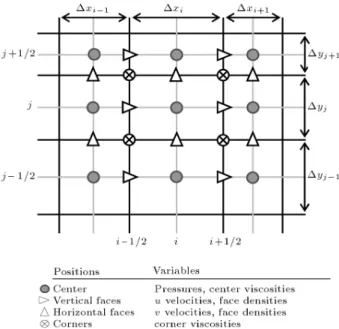
For this model, a non-uniform staggered grid is consid-ered as shown in Figure 1. In this type of grid, three types of position are validated as the centers, corners and faces of control volumes.

In this grid, pressure as a scaler variable is located at the center of the cell, densities are located in the faces, viscosities are located at the centers and corners. Vertical and horizontal components of velocities are located on the faces of the cell. The position of the density is very important and eective in two phase ow modeling. It is shown that by using the FGVT algoritm for the colour function advection solution, the high accuracy computations of densities and viscosities are possible in real positions.

The variation of spatial steps in non-uniform grid needs more attention for protection against any excessive error due to this variation.

Interface Reconstruction and Advection of Color Function

As shown in the 1st step of the two-uid simulation, the interface must be captured by advection of the color function in the ow eld. In the common volume of uid approach, the distribution of phases is represented by volume fraction Ci;j of the liquid phase in cell

(i; j). The PLIC (Youngs') method uniquely denes the interface in each cell with 0 < C < 1 by a slope segment which is perpendicular to a given normal, n, to the interface (n = r:C). The main idea of interface

Figure 1. Staggered grid and types of positions and variables in non-uniform grid.

construction and advected uxes of color function is shown in Figure 2 in a control volume.

According to the Youngs' method, the interface normal (n) is initially calculated at each corner of the cells as the gradient of the color function. In this scheme, components of n are computed by neighboring cells for a non-uniform grid as follows:

n_i+1

2;j+12 =[(Ci+1;j+1 Ci;j+1)yj

+(Ci+1;j Ci;j)yj+1]=

((yj+ yj+1):xi+1 2)i

+[(Ci+1;j+1 Ci+1;j)xi

+(Ci;j+1 Ci;j)xi+1]=

((xi+ xi+1):yj+1

2)j: (6)

The cell-centered normal is calculated by averaging these corner normals.

ni;j=1₄(ni+1

2;j+12 + ni 12;j+12 + ni+12;j 12+

n_i 1

2;j 12): (7)

At each time step, after constructing the interface, the ux of the color function is computed by the scheme that is shown in Figure 2. The color function in the new time step is calculated by the FCT-VOF method [15]. At the beginning, set Vn

i;j = xi:yj, then for the

x-sweep of the mesh, the following calculations should be set down:

e

Ci;j= Ci;jn Vi;jn (Fi+x 1 2;jF

x i 1

2;j);

Vn+12

i;j = Vi;jn ty(ui+1

2;j ui 12;j);

Figure 2. Linear interface construction and advected ux from right face of control volume.

Cn+12

i;j = ~Ci;j=Vn+

1 2

i;j : (8)

The y-sweep is calculated similarly. After these two direction sweeps, V should be set again equal to x:y.

For surface tracking with higher resolution, Rud-man [16] proposed the FGVT method. In this method, surface tracking is solved on a grid with half the size of a hydrodynamic grid. This methodology leads to higher accuracy in interface tracking, higher accuracy in density estimation in the face of cells and superior accuracy in the advection of momentum. In Figure 3, the rened grid and new numbering in the FGVT method are shown. In this scheme, each main cell is divided into 4 equal ne cells. Each ne cell has a parameter as color function ci;j. In the non-uniform

grid, the size of the ne grid is obtained as follows: x2i= x2i+1=1₂xi;

y2j = x2j+1= 1₂yj: (9)

Since in the ne grid approach there are no parameters such as velocities for volume tracking computation, these parameters must be obtained by interpolation from the coarse grid. In this interpolation, the main attention must be paid to mass conservation. Thus, a simple interpolation is selected for velocities on a ne grid given by Equation 10. This method is also illustrated in Figure 4.

(u_2i+1

2;2j)FG= ui+12;j;

(u2i 1

2;2j)FG= 0:5(ui+12;j+ ui 12;j): (10)

Figure 3. FGVT rened grid and usage of new numbering of ne cells.

Figure 4. Velocities of a coarse grid cell (solid line) and ne grid cells (dashed line).

Using the color function in the ne grid, some param-eters can be solved easily as follows:

_i+1

2;j = 0:5((2i;2j+ 2i;2j 1)xi

+ (2i+1;2j+2i+1;2j 1)xi+1)=(xi+xi+1):

(11) At the rst step after computation of middle color function c _{in the ne grid, it is easy to compute}

in the vertical and horizontal faces of the cells. Advection of Momentum

One of the major problems in two-uid modeling is the high density variation at the interface of the uids. This large density variation makes diculties for momentum conservations. An additional consideration is that reasonable estimates of ux densities must be made to ensure that momentum uxes are consistent with mass uxes.

For this purpose, a second order scheme is used for solution of the momentum advection as follows:

(u) _(u)n

t + r:(uu) = 0: (12)

An assumption, with good arguments for two-uid modeling, is made which asserts that although density and hence momentum may be discontinuous across an interface, the velocity eld varies smoothly. Due to this discontinuity, the use of high order standard dif-ferencing techniques for momentum advection will yield unstable solutions and rapidly destroy the solution, since the Taylor expansion of density is not valid in the neighborhood of the discontinuity.

In recent work, momentum advection is based on the fully multidimensional Zalesak Flux Corrected Transport algorithm (ZFCT) with two signicant dif-ferences [16]:

1. The calculation of densities and momentum uxes at the faces of the control volume,

2. The min:max values used in the ux limiter. For computation of momentum uxes in an x di-rection at the 1st step of advection, two types of control volume must be considered for solving Equations 13 and 14.

(u) _(u)n

t + r:(uu) = 0; (13)

(v) _(v)n

t + r:(vu) = 0: (14)

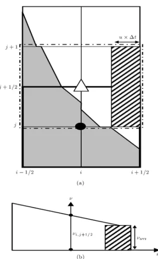
In Figure 5a, the control volume for Equation 13 is shown. For solving (u)_{, the value of (v)}n _{and the}

ux of (u)that crosses the vertical faces of the control volume must be known. However, (u)n _{is known}

from the last computations or initial conditions. As shown in Figure 5, for high accuracy computation of the momentum ux (hatched area), a good estimate of velocity and density in the hatched area must be known. In a standard MAC algorithm, these densities are obtained using linear or bilinear averages of nearby C-values and Equation 4. In FGVT, an estimate of the average density of the uid crossing each side of a momentum control volume can be made using the information obtained from the advection of c-values on the ne grid. Considering the x-momentum

Figure 5. (a) Control volume of momentum of u in x direction (dash-dotted line), ux of momentum crossing the vertical face of the control volume (hatched area); (b) linear distribution of u.

control volume centered on (i 1=2; j) and shown in Figure 5, the averaged density of x-momentum ux m is computed by F2i 0:5;2jx and F2i 0:5;2j 1x using

Equation 15, which are uxes of the advected color function in the ne grid. It should be mentioned that Fx

m is the mean void fraction of the uid crossing the

face, i, of a momentum control volume in a time step, as shown in Figure 5.

m= (Fmx:1+ (1 Fmx):2);

Fx m=

Fx 2i 1

2;2j + F

x 2i 1

2;2j 1

ui;j:t:yj ; (15)

2nd order accuracy is used for good estimation of the velocity of the uid being uxed across the face of the control volume. In this method, a linear distribution for u velocity is assumed for the upwind control volume, as shown in Figure 5, and is computed by the following equation:

u = u_i 1

2 + si 12:(x xi 12);

s_i 1 2 =

un i+1

2;j u

n i 3

2;j

xi 1+ xi : (16)

By this distribution, the averaged velocity of the x-momentum ux is computed as follows:

uavr=ui 1

2 + 0:5(xi 12 ui;jt)si 12 if ui;j>0;

ui;j= 0:5(ui+1

2;j+ ui 12;j): (17)

The computed u and uavrfrom the above equations are

used in x-momentum computations as; (u)

i 1 2 =(u)

n i 1

2 (ux

ux

i uxuxi 1)=

(xi 1

2yj); (18)

uxux_i = m:uavr:ui;jt:yj: (19)

The same methodology as above is used for solving Equation 14. In Figure 6, the control volume of the y-momentum advected by horizontal velocities is shown. This control volume is around the v-velocity position. At this step, the averaged density of the crossing ux is computed by Equation 20, and the ux is computed by Equation 21:

m= (Fmx:1+ (1 Fmx):2);

Fx m=

Fx 2i+1

2;2j+ F

x 2i+1

2;2j+1

u_i+1

2:t:yj+12

; (20)

uxvx_i+1

2;j+12 = m:vavr:ui+12; j +

1

2:t:yj+1

Figure 6. (a) Control volume of momentum of v in x direction (dash-dotted line), ux of momentum crossing the vertical face of the control volume (hatched area); and (b) linear distribution of v.

where the averaged v-velocity is computed from Equa-tion 17 and u_i+1

2;j+12 is obtained by the linear averaging

of two u-velocities in (i + 1=2; j) and (i + 1=2; j + 1) positions.

In the Rudman method [16] for higher-order accuracy, ux limiting is used. Once low- and high-order uxes have been estimated, anti-diusive uxes are calculated and limited in a similar way to the fully multidimensional Zalesak procedure. In the Rudman method, for higher-order ux computation, the averaged velocity in the ux area is computed on vertical faces. However, in this paper, the velocity is obtained in the middle of the ux by assuming a linear variation of velocity. For advection of the color function and momentum by v-velocities, the above steps are repeated by proportional control volumes.

Diusion by Viscosity

In the 2nd step of the main methodology, as used in this paper, the Reynolds stresses must aect the momentum equation. The eect of Reynolds stresses

is given by the following:

(u) _(u)

@t =

@ @x

@u_@x

+_@y@

@u_@y

: (22) Figure 7 helps to dene the numerical solution of Equation 22. In this gure, the best position of equivalent viscosity is shown by multiplied circles in cell corners and lled circles at the center of the cells.

The required position of equivalent viscosity is also given in the following equation:

((u) _(u))

i+1 2;j

@t =

1 x_i+1

2

i+1;j

u_i+3

2;j ui+12;j

xi+1

i;j

u_i+1

2;j ui 12;j

xi

+_y1

j i+12;j+12

ui+1

2;j+1 ui+12;j

y_j+1 2

_i+1 2;j 12

u_i+1

2;j ui+12;j 1

y_j 1 2

!

: (23)

For elimination of averaging, using the FGVT algo-rithm, the laminar (and eddy) viscosities are computed in both positions. By the implicit Crank-Nicolson method, diusion equations are solved in the x and y-momentum. After the diusion steps u_{and vare}

updated as u _{and v, respectively.}

Figure 7. Local grid for Reynolds stresses computation and location of viscosities.

Laminar and Turbulent Viscosity

To use the model under both laminar and turbulent conditions, an equivalent viscosity as = l+tis used

in the nal formulation where land tare laminar and

turbulent viscosities, respectively.

Under high Reynolds conditions, a realizable Reynolds stress algebraic equation model [18] is used for the Reynolds stress term. The latter model has signicantly improved the predictive capability of k " based models especially for ows involving strong shear layers. The equations for these models are:

@k

@t + u:rk =r:

1

(l+ t=k)rk

+1

(Gk+ Gb "); (24)

@"

@t + u:r" = r:

1

(l+ t=")r"

+1C1"_k"(Gk+ C3"Gb)

C2""

2

k; (25)

where, eddy viscosity is computed from: t= Ck

2

" ; (26)

where k and " are turbulent kinetic energy and dissipa-tion rate, respectively, the turbulent Prandtl numbers for k and " values are k = 1, " = 1:3, and the

coecient values are C1"= 1:44 and C2"= 1:92. Also,

Gk is the generation of turbulent kinetic energy due

to mean velocity gradients and Gb is the generation of

turbulent kinetic energy due to buoyancy. Gk= u0iu0j@u_@xj

i

=

u0_u0@u

@x + u0v0 @u @y + @v @x

+ v0_v0@v

@y

;

S =pGk=t; (27)

Gb=_Pt rt

gx_@x@ gy@_@y

; Prt= 0:85: (28)

In the realizable model, estimation of the Reynolds stress tensor, u0

iu0j, can be written as:

u0

iu0j=2₃kij C(k2=")2Sij

+2C2(k3="2)( Sikkj+ Skjik); (29)

where: Sij =1₂

@ui

@xj +

@uj @xi 1 3 @uk

@xkij; (30)

ij= 1₂

_@u i @xj @uj @xi : (31)

In the standard k " model C = 0:09 and C2 = 0.

However, for the algebraic model, these coecients are: C=_{6:5 + A(Uk=")}1 ;

C2=

q

1 9SijSijC(k=")2

1 + 6 pSijSij(k=")pijij(k="); (32)

U =pSijSij+ ijij;

A =p6 cos

1 3arccos

p 6W; W = SijSjkSki

(SijSij)

3

2: (33)

For computation of the buoyancy eect in Equation 29, a spatial method is used:

Gb=2_P t rt gx

_i+1

2;j i 12;j

x_i+1

2;j+ i 12;j

gy

_i;j+1

2 i;j 12

y_i;j+1

2 + i;j 12

!

: (34)

The third constant of the k " model is computed by C3"= tanh jvg=ugj where vgis the ow velocity parallel

to the gravitational vector and ug is perpendicular to

the gravitational vector [19].

Turbulent conditions in separated ow are af-fected strongly by the interface. The interface limits the vorticity sizes in the vicinity of the separation surface between high and low density uid. These limitations are due to some additional forces such as surface tension and buoyancy.

For computation of laminar viscosity in the center and corner of cells, initially, cell-centered viscosities in the ne grid are computed using the computed color function as follows:

FG

l;2i;2j = cn+12i;2j1+ 1 cn+12i;2j

2; (35)

where FG

l;2i;2j is the equivalent laminar viscosity in

cell centers of the ne grid. Rudman has proposed a harmonic averaging for equilibrium viscosity in the

cell-corner, given by Equation 36. While this equation is only used in the x-momentum equation; for the y-momentum Equation 37 is used.

x i+1

2;j+12=

FG

2i;2j+FG2i+1;2j

: FG

2i;2j+1+FG2i+1;2j+1

= FG

2i;2j+FG2i+1;2j+FG2i;2j+1+FG2i+1;2j+1

; (36) y_i+1

2;j+12=

FG

2i;2j+FG2i;2j+1

: FG

2i+1;2j+FG2i+1;2j+1

= FG

2i;2j+FG2i+1;2j+FG2i;2j+1+FG2i+1;2j+1

: (37) The above averaging is aected by the variation of spatial steps and by the weight of the ne grid cell area in the non-uniform grid. Equation 38 introduces computation of the cell-center laminar viscosity.

l;i;j= 1₄(FGl;2i 1;2j 1+ FGl;2i;2j

+ FG

l;2i;2j 1+FGl;2i 1;2j): (38)

Considering Eects of the Surface Tension and Gravity

In our formulations, body forces, including the ef-fects of gravity accelerations and surface tensions, are considered. At this step, velocities in momentum equations are updated as:

us_{= u+ g}

xt + 1 i+1

2;j

F_x;i+1 2;jt;

vs_{= v+ g}

yt + 1 i;j+1

2

F_y;i;j+1

2t; (39)

where Fxand Fyare components of the Fssurface force

arising from interfacial eects.

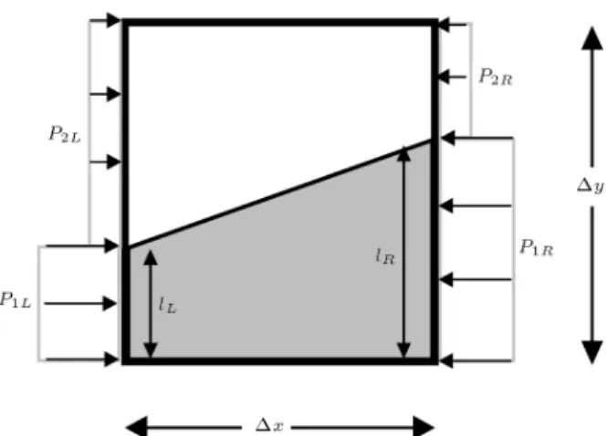
The Pressure Calculation, based on the Interface Location (PCIL) method, presented by Shirani et al. [20], is used for surface tension. This method is based on calculation of the pressure force at each interfacial cell face using the exact pressure due to the portion of the cell face that is occupied by each uid. In the PCIL method, interface forces are computed as:

Fs= Hsn = Hnjr ~_[C]Cj; (40)

where is the equivalent surface tension coecient, is the interface curvature, n is the unit normal vector of the interface and H is a non-dimensional parameter that denotes the location of the interface at the cell side (HR= lR=y as in Figure 8). The sign of (or tilda)

denotes a ltered or smoothed value and the square brackets denote the dierence between the maximum

Figure 8. An interface cell with cell face pressures along the x-axis.

and the minimum values of the function inside the brackets.

In a turbulent ow condition, due to the existence of a uctuation of velocities and pressure, the behavior of the surface tension is dierent. Shirani et. al. [17] proposed a new method for obtaining this term under turbulent conditions. They show that the unresolved high-frequency small-scale uctuations of curvature in a turbulent ow can be represented by increasing the mean curvature, , by a factor of pt=, due to

turbulence eects with the proper coecient. It shows that the surface tension force in a turbulent ow is increased by a factor ofpt=.

This methodology is used for general conditions of laminar and turbulent ows as follows:

= 0+ t= 0

1 + Cp

p t=

; (41)

where 0is the molecular surface tension coecient, t

is the turbulent surface tension coecient and Cpis the

model constant to be determined due to calibration. Pressure and Velocity Computing

At this step, continuity and remained momentum equations are discretized as:

r:u = 0 )y:un+1 i+1

2;j u

n+1 i 1

2;j

+ x:vn+1

i;j+1 2 v n+1 i;j+1 2

= 0; (42)

@u

@t + r:P = 0 ) 8 < : _i+1 2;j un+1 i+1 2;j u

s i+1

2;j

=t: Pn+1

i+1;j Pi;jn+1

=x _i;j+1 2 vn+1 i;j+1 2 v s i;j+1 2

=t: Pn+1

i;j+1 Pi;jn+1

=y (43) By overlaying Equation 43 by Equation 42, the dis-cretized Poisson equation is obtained.

The Poisson equation can be written as A Pn+1 _{= B. The system of linear equations is solved}

directly by the LU (Lower/Upper triangular decom-position) method, which is optimized for a bounded matrix, and the pressures at the new time steps are obtained. After computing the pressure using Equation 43, new velocities in the new time step are obtained.

RESULTS

In order to check the validity of the numerical model, a number of test cases have been considered. These in-clude verication tests for the volume tracking method and two-phase ow models.

Interface Tracking by VOF in a Convergent-Divergent Channel

In this test case, a channel is considered where the center line coincides with the x-axis of the coordinate system and function f(x) species the distance between the channel wall and the center line. The velocity eld is derived from the assumption that the component, u, parallel to the center line has a parabolic prole at every cross-section of the channel. The only solenoidal velocity eld (u; v) having a parabolic prole of u at every cross section of the channel is given by:

u = 1

y f(x)

2! ₁

f(x); v = 1

y f(x)

₂! y (f(x))2

d

dxf(x); (44)

and the channel prole is given by: f(x) = 1 a exp

1 2xb

2

;

a = 0:75; b = 0:5: (45)

The computational domain is the rectangle [ 2:5; 2:5] [ 1:0; 1:0] divided into 250 100 computational cells, implying square computational cells of side length x = y = 0:02. For the initial condition of the interface, a bubble is located at the point (1.95, 0) and its radius is 0.5.

The nal state is considered at time t = 2020 t. The time step, t, corresponds to the Courant number, C = 0:3 or t = 0:001465.

The results of FGVT-VOF are shown in Figure 9 for the initial t = 0, t = 1220 t and t = 2020 t. Figure 10 shows the result of the test procedure when applied to the following dierent interface tracking methods:

Figure 9. Results of convergent-divergent channel modeling by FGVT-VOF method; circles are exact solutions, solid lines are FGVT solutions.

Figure 10. Results of convergent-divergent channel modeling by dieren methods. (1) Level Set method; (2) Unsplit PLIC VOF; and (3) FGVT VOF method.

1. Level Set [21],

2. Unsplit PLIC-VOF [22],

3. FGVT-VOF method used in this paper.

Results show that VOF methods have superior volume conservation properties, but are liable to develop small-scale topological irregularities like the outward bend of the two \ne tips" in the nal state. However, using the ner grid in the FGVT method reduces these irregularities.

Lock Exchange Test Case

The lock exchange ow is a well-known test case to verify the modeling of density currents. The name of this test case originates from the practical engineering problem concerning the intrusion of a salt water wedge under fresh water when a lock gate is opened at the mouth of a fresh water channel leading to the sea. This test case is selected for verication of a two phase ow model. Two incompressible uids with slightly dierent density conned in a rectangular basin with impermeable walls, are initially divided by a very thin wall as shown in Figure 11. Under the initial condition, the left half of the domain is lled by uid of a higher density and the right half by uid of a lower density.

Under equilibrium conditions, the velocity of the density current can be estimated from energy conser-vation considerations as:

Uc=

r

0:52 1

2+ 1gH: (46)

The model conguration is set to match that of Jankowski [23] with channel length L = 30 m and depth H = 4 m. The horizontal and vertical resolutions are x = 0:2 m, y = 0:2 m and CFL = 0.1. Initially, the left and right halves of the basin are occupied by water of density 2= 1000:722 kg/m3and

1= 999:972 kg/m3, respectively.

In Figure 12, the results of a two phase ow modeling and an ordinary density current simulation for a lock exchange problem are shown. In Figure 13, the time series current speed in the middle of a channel at points at the surface and the bottom are shown. Figure 12 shows agreement between these two types of modeling, but two phase modeling is the same as the analytical solution otherwise ordinary solutions have some diusion errors. Also, in Figure 13, it can be seen that two phase ow modeling is fully symmetric. These results show that the model can be used for density

Figure 11. Lock exchange problem.

Figure 12. The results of lock exchange problem after 100 sec. (a) Simulated by two phase ow modeling in present work; and (b) Ordinary density current simulation [23].

Figure 13. The lock exchange ow wedge speed (density current) time series for points at surface and bottom (up and down) in middle of the basin.

current simulations if immiscibility is considered in phenomena.

Dam Break Modeling

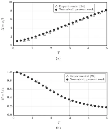
For two-phase ow modeling with high density vari-ations, the experimental data of Martin and Moyce are used [24]. Figure 14 shows the initial conditions of a column of water (a) and the time evolution (b) of a dambreak test case. In Figure 15, the numerical results, as a non-dimensional (a) surge front position and (b) height of water column, are compared to the experimental data. Reasonable agreement between the numerical simulation and the experiments is observed, as shown in Figure 15.

Figure 14. (a) Initial condition for column of water and (b) results of two phase ow modeling at dierent stages on a non-uniform structured grid for validation of the two phase ow model.

Figure 15. Comparison of non-dimensional results of 2D numerical model with the experimental data [24] at dierent non-dimensional times. (a) X-surge front position; and (b) H-height of water column collapsing.

Dam Break Modeling with Obstacle

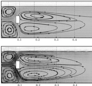
For verication of the capabilities of interface-capturing methods, the dam-break problem with an obstacle is considered as a standard test case for computing free-surface ows. As shown in Figure 16, the barrier holding back the uid is suddenly removed for the dambreak example. As water ows to the right, it hits an obstacle thus owing over it and hitting the opposite wall. The conned air escapes upwards as the water falls to the oor on the other side of the obstacle. The initial conditions and dimensions are shown in Figure 16 and the numerical modeling is shown for dierent time steps in Figure 17. Also, as illustrated in Figure 18, the numerical results are compared well

Figure 16. Dimensions and initial condition for dambreak test case with obstacle.

Figure 17. Results of two phase ow modeling at dierent time steps from 0 to 0.5 sec.

Figure 18. Comparison of results of 2D numerical model with the experimental data of Koshizuka et al. [25] and numerical results of Mujaferija et al. [26] at two stages (a) 0.2 sec. and (b) 0.4 sec.

with the experiments of Koshizuka et al. [25] and the numerical predictions of Muzaferija and Peric [26] at the two time steps of t1= 0:2 sec and t2= 0:4 sec after

breaking. Settling Tank

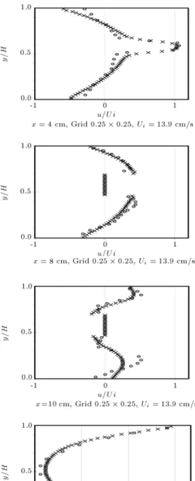
A nal test case is selected for verication of the turbulent modeling under a two phase ow condition in which turbulent modeling is undertaken in the inlet region of a rectangular laboratory scale settling tank. The experimental results of this case were presented by Lyn and Rodi [27] and the details of it are shown in Figure 19. Eects of the presence of sediments are not considered. and the average velocity, U, is 1.6 cm/s.

Two types of computational grid with 0.5 0.5 and 0.25 0.25 cm spatial size are used. In both types of grid, after the recirculation zone, the grid size is increased. The global results of this simulation are shown in Figure 20. In 5 positions, namely at 4, 8, 10, 18, 30 and 40 cm which are shown in Figure 20, the vertical prole of the horizontal velocity is compared with experimental and numerical results. The results of the two types of grid are shown in Figure 21, and are compared with the experimental data of

Figure 19. Details of settling tank and deector.

Figure 20. Results of settling tank modeling by turbulence two phase ow model on two dierent computational grids 0.5 0.5 (top) and 0.25 0.25 (down).

Lyn and Rodi [27]. The results show a fairly good agreement with experimental data without considering any specic assumption in the two phase modeling. These types of modeling are usually performed with single phase modeling and for turbulent models with symmetric conditions on a free surface as well.

CONCLUSIONS

In this paper, a numerical model for a two phase ow simulation under general conditions such as laminar and turbulent, is presented. The FGVT method is used for computation of the interface tracking and is coupled with the second order advection solution of momentum equations. Discretization of a second order coupled method without any limiters is presented for momentum advection under high density variation conditions. Equivalent laminar viscosity at two types of position in a computational grid is used. The

Figure 21. Comparison results of computational modeling with two grid sizes and experimental results [27], in vertical proles of non-dimensional velocity in settling tank.

k " model is used for turbulent simulation. For the verication of interface tracking one test case is used and for hydrodynamic modeling three test cases are selected, i.e. exchange ow and a dam break with and without obstacles. The results of modeling are tested with analytical or experimental results. All results compare well with other experimental, analytical and numerical results.

NOMENCLATURE

c volume function of liquid phase in ne grid

C volume function of liquid phase in main grid

uxux _{ux of momentum of u in x direction}

Fx _{ux of advected colour function in x}

direction in n grid Fx

m mean void fraction of uid crossing the

velocity control volume Fs body forces of surface tension

gx; gy components of acceleration vector in x

and y direction

Gk generation of turbulent kinetic energy

Gb generation of turbulent kinetic energy

due to buoyancy

H non-dimensional location of the interface at cell side

k turbulent kinetic energy

n interface normal

P pressure

Sij strain tensor

u; v local velocity components in x and y direction

uavr averaged velocity of x-momentum ux

Greek Symbol

x; y spatial steps of grid in x and y direction

t time step

V volume or area of cell " dissipation rate of energy

interface curvature

1; 2 uid viscosity of rst and second phase

1; 2 uid density of rst and second phase

f averaged density of x-momentum ux

k; " Prantle numbers for turbulent k and "

surface tension coecient

Superscript

n pesent time step

n + 1 view time step

s aected by body forces

aected by advection in x direction aected by advection in y direction

aected by diusion

0 _{Reynolds uctuating part}

Subscript

i; j cell numbering in main grid 2i; 2j cell numbering in ne grid

F G cine grid

L; R; C left, right, center

avr averaged

t turbulence

l laminar

REFERENCES

1. Hirt, C.W. and Nichols, B.D. \Volume Of Fluid (VOF) method for the dynamic of free boundaries", Journal of Computational Physics, 39, pp. 201-225 (1981). 2. Harlow, F. and Welch, J. \Numerical calculation of

time-dependent viscous incompressible ow of uid with free surface", The Physics of Fluids, 8(12), pp. 2182-2189 (1965).

3. Popinet, S. and Zaleski, S. \A front-tracking algorithm for accurate representation of surface tension", In-ternational Journal for Numerical Methods in Fluids, 30(6), pp. 775-793 (1999).

4. Unverdi, S.H. and Tryggvason, G. \A front-tracking method for viscous, incompressible, multi-uid ows", Journal of Computational Physics, 100, pp. 25-37 (1992).

5. Osher, S. and Sethian, J.A. \Fronts propagating with curvature-dependent speed: Algorithms based on Hamilton-Jacobi formulations", Journal of Computa-tional Physics, 79(1), pp. 12-49 (1988).

6. Enright, D., Losasso, F. and Fedkiw, R. \A fast and accurate semi-lagrangian particle level set method", Computers and Structures, 83, pp. 479-490 (2005). 7. Sussman, M. \A second order coupled level set and

volume-of-uid method for computing growth and collapse of vapor bubbles", Journal of Computational Physics, 187, pp. 110-136 (2003).

8. Van Der Pijl, S.P., Segal, A. and Vuik, C. \A mass-conservation level-set (MCLS) method for modeling of multiphase ows", ISSN 1389-6520, Report 03-03 of the Department of Applied Mathematical Analysis, Delft (2003).

9. Tanguy, S., Menard, T., Berlemont, A. \A level set method for vaporizing two-phase ows", Journal of Computational Physics, 221, pp. 837-853 (2007). 10. Fukagata, K., Kasagi, N., Ua-arayaporn, P. and

Hi-meno, T. \Numerical simulation of gas-liquid two-phase ow and convective heat transfer in a micro

tube", International Journal of Heat and Fluid Flow, 28, pp. 72-82 (2007).

11. Rider, W.J. and Kothe, D.B. \Reconstructing volume tracking", Journal of Computational Physics, 141, pp. 112-152 (1998).

12. Aulisa, E., Manservisi, S. and Scardovelli, R. \A mixed markers and volume-of-uid method for the reconstruction and advection of interfaces in two-phase and free-boundary ows", Journal of Computational Physics, 188, pp. 611-639 (2003).

13. Youngs, D.L. \Time-dependent multi-material ow with large uid distortion", in Numerical Methods for Fluid Dynamics, edited by Morton, K.W. and Baines, M.J., Academic Press, New York, pp. 273-285 (1982). 14. Ashgriz, N. and Poo, J.Y. \FLAIR: Flux line-segment model for advection and interface reconstruction", Journal of Computational Physics, 39, pp. 201-225 (1991).

15. Rudman, M. \Volume-tracking methods for interfacial ow calculations", International Journal for Numeri-cal Methods in Fluids, 24, pp. 671-691 (1997). 16. Rudman, M. \A volume-tracking method for

incom-pressible multiuid ows with large density varia-tions", International Journal for Numerical Methods in Fluids, 28, pp. 357-378 (1998).

17. Shirani, E., Jafari, A. and Ashgriz, N. \Turbulence models for ows with free surfaces and interfaces", AIAA Journal, 44(7), pp. 1454-1462 (2006).

18. Shih, T.H., Zhu, J. and Lumley, J.L. \A new Reynolds stress algebraic equation model", Computer Methods in Applied Mechanics and Engineering, 125(1), pp. 287-302 (1995).

19. Henkes, R.A.W.M., Van der Flugt, F.F., Hoogen-doorn, C.J. et al. \Natural convection ow in a

square cavity calculated with low-Reynolds-number turbulence models", International Journal Heat Mass Transfer, 34, pp. 1543-1557 (1991).

20. Shirani, E., Ashgriz, N. and Mostaghimi, J. \In-terface pressure calculation based on conservation of momentum for front capturing methods", Journal of Computational Physics, 203, pp. 154-175 (2005). 21. Sussman, M., Almgren, A.S., Bell, J.B. and Colella,

M. \An adaptive level set approach for incompressible two-phase ows", Journal of Computational Physics, 148, pp. 81-124 (1999).

22. Meier, M., Yadigaroglu, G. and Andreani, M. \Nu-merical and experimental study of large steam-air bubbles injected in a water pool", Nuclear Science and Engineering, 136, pp. 363-375 (2000).

23. Jankowski, J.A. \A non-hydrostatic model for free surface ows", Ph.D. Thesis, University of Hannover (1999).

24. Martin, J.C. and Moyce, W.J. \An experimental study of the collapse of liquid columns on a rigid horizontal plane", Philosophical Transactions of the Royal Society of London, 244, pp. 312-324 (1952).

25. Koshizuka, S., Tamako, H. and Oka, Y. \A particle method for incompressible viscous ow with uid frag-mentation", Computational Fluid Dynamics Journal, 4, pp. 29-46 (1995).

26. Muzaferija, S. and Peric, M. \Computation of free surface ows using tracking and interface-capturing methods", in Nonlinear Water Wave Inter-action, O. Mahrenholtz, M. Markiewicz, Eds., Chap. 2, pp. 59-100, WIT Press, Southampton (1999). 27. Lyn, D.A. and Rodi, W. \Turbulence measurements in

model settling tank", Journal of Hydraulic Engineer-ing, 116(1), pp. 3-21 (1990).