Narx Based Short Term Wind Power Forecasting Model

ISSN: 2252-8938  129

Narx Based Short Term Wind Power Forecasting Model

M. Nandana Jyothi1, V. Dinakar2, N. S S Ravi Teja3

1

Department of Electrical and Electronics Engineering, Acharya Nagarjuna University, Andhra Pradesh, India

2,3

Department of Electrical and Electronics Engineering, K L University, Andhra Pradesh, India

Article Info ABSTRACT

Article history:

Received August 4, 2015 Revised Oct 8, 2015 Accepted Nov 14, 2015

This paper contributes a short-term wind power forecasting through Artificial Neural Network with nonlinear autoregressive exogenous inputs (NARX) model. The meteorological parameters like wind speed, temperature, pressure, and air density are considered as input parameters collected from KL University area and the calculated generated power as output parameters of neural network to predict the wind power generation. Based on hybrid forecasting technique a code is developed in MATLAB at different hidden layers and delay times.

Keyword: ANN

Hybrid method Narx

Netc

Wind power forecasting Copyright © 2015 Institute of Advanced Engineering and Science.

All rights reserved.

Corresponding Author: M. Nandana Jyothi,

Department of Electrical and Electronics Engineering, Acharya Nagarjuna University,

Guntur, Andhra Pradesh, 522502- India. Email: [email protected]

1. INTRODUCTION

In the present day scenario the need for electrical power is growing in an exponential manner. The fuel reserves for the electrical power generation through conventional methods are depleting at a very faster rate and are causing severe harmful effect on the environment. According to the Global Wind Energy Outlook 2014 by Global Wind Energy Council (GWEC) power sector is the sole emitter of about 40% of the carbon dioxide and 25% of all the green house gases.

The better solution that addresses most of the problems that arises because of the fossil fuels is the usage of renewable energy. Among all the renewable energies wind energy is the most promising and cheaper to operate. But there is a huge demand for the electrical energy which is partly shared by the non-conventional energy resources. GWEC in its recent publication stated that the wind energy could reach 2000GW by 2030.

But the major hindrance for the expansion and integration of the wind power to the grid is the high volatile and intermittent nature of the wind power. Because of these natures of wind power it is very difficult to integrate to the grid and schedule the power. To overcome the stated problems wind power forecasting is the best solution. Wind power forecasting model helps the power system operators in power scheduling, dispatch, grid security, system operation and maintaining the reserve capacities. There are different forecasting methods according to different time horizions which are very short term forecasting method in this minutes to hours time horizon is considered, short-term forecasting method is hours to days time horizon is considered, long –term forecasting method is considered as day to months are considered [1-5].

1.1. Over view of the present wind forecasting methods

There are various forecasting methods developed to predict wind speed and or power, which are presented as the following tabular column:

Table 1. Wind Forecasting Methods and their Application [1]-[6]

Forecasting method Sub class Technique Advantages Dis-advantage

Persistence method - P(t+k) = p(t)

Bench mark approach for Very short term wind power forecasting.

Reliability decreases as time lapse increases.

Physical approach Numerical Weather

Prediction(NWP)

Solve complex

mathematical models using large

meteorological data is collected to develop patterns

It is reliable for medium to long term forecasting.

Need large number of computations (super computers needed).

Statistical approach

Artificial Neural Network (ANN)

Tune the network with the help difference between actual data and measured data

Not completely based on predefined equations

Data measurement should be accurate for proper training of the network.

Time series models

Hybrid structures NWP&ANN

Combination of

forecasting methods is used to improve the efficiency of forecasting.

It is reliable for very short term forecasting.

Data measurement should be accurate for proper training of the network.

The predication carried out in this paper uses the hybrid structures. Statistical data is collected from the Energy Department of KLUniversity, Andhra Pradesh which consists of 720 hours data of which 672 hours data is used for training and 48 hours data is used for prediction and also the physical laws are taken into account for the calculation of power generation. The developed model is based on the non-linear auto regressive with exogenous input (narx) tool which trains the ANN for the time series. The input parameters taken into consideration are wind speed, temperature, pressure, air density and the output parameter is generated power. Mean square error and root mean square error are calculated from the predicted and known results.

1.2. Calculation of wind power from the data

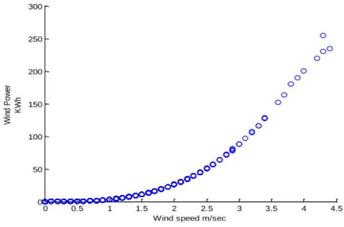
The wind power generated by the turbines depends upon the factors like wind speed, ambient temperature, wind pressure, air density. Among all the factors wind speed and air density dominates the power generated. Wind power generated is known by

(1)

Where P-Wind power generated

Ρ-Air density at the given temperature A-Area swept by the turbine blades V-Wind speed

Wind power generated is highly affected by the air density and the wind speed; as the area swept by the turbines blades remain constant for a taken turbine [5]. The data is collected from Energy Department of K L University, vaddeswaram area for a time span of one month which comprises of wind speed, ambient temperature, and air pressure. The air density in the considered area is not known. For the density calculations vapour pressure is required according to the formula [5]

( ) (

) (2)

Where ρ- Air density at the given temperature D- Air density at absolute temperature T- Given temperature

B- Barometric (atmospheric) pressure

e- Vapour pressure of the air at the given temperature

All the data required for the density calculation is present except the vapour pressure. In a closed system the pressure exerted by a vapour in thermodynamic equilibrium at a given temperature is the vapour pressure. Vapour pressure is calculated using the Clausis-clapeuron relation.

(

) (

) (

) (3)

Where P1, P2 – The vapour pressures at temperatures T1, T2 respectively

𝝙Hvap – Enthalpy of vapourization of liquid

R- Real gas constant (8.314J)

T1- Temperature at which the vapour pressure is known

T2- Temperature at which the vapour pressure to be calculated

Take T1 and P1 at STP conditions and P2 is the vapour pressure to be calculated at which the temperature is T2. By this formula vapour P2, ‘e’ in the density calculation is obtained. Air density is then calculated by the stated formula. The data required for the calculation of power genration is obtained and the power that can be generated by using all these parameters is calculated by ignoring the operational losees of turbine.

Figure 1. Diagramtical Representation of Wind Speed vs Power Generated

2. RESEARCH METHOD

2.1. Artificial Neural Network (ANN)

Artificial neural networks are the neural networks derived from the inspiration of biological neural networks (animal central nervous system). These artificial neural networks are used to take logical decisions based on the inputs. ANN can deal with non-linear and complex problems in terms of classification or forecasting by extracting the dependence between variables through the training process. So the ANN based method is an appropriate method to apply to the problem of forecasting wind power because it is directly proportional to wind speed which is highly intermittent in nature. Among the available methods using artificial neural networks the NARX, a dynamic recurrent method, is used to solve the time series problem [7-10].

2.1.1. ANN training

One of the key elements of neural networks is their ability to learn. A neural network is a complex adaptive system, which means it can change its internal structure based on the inputs and targets. These ANNs need to be trained for doing a particular task [10-14]. There are three types of training paradigms to train the artificial neural network and are as follows:

1. Supervised training: It is the process of providing the network with a series of sample inputs and comparing the output with the expected response. The training continues until the network is able to provide the expected response. The proposed work is supervised training with back propagation technique.

2. Unsupervised training: In this method of training, the input vector and the target output is not known. The network may modify in such a way that the most similar input vector is assigned to the same output unit.

3. Reinforcement training: It is the process of training the network in the presence of a teacher but in the absence of target vector. The teacher gives only the answer whether it is correct (1) or wrong (0).

0 0.5 1 1.5 2 2.5 3 3.5 4 4.5

0 50 100 150 200 250 300

Wind speed m/sec

W

in

d

P

ow

er

K

W

2.1.2. Non linear Auto Regressive with exogenous input (NARX)

The nonlinear autoregressive network with exogenous inputs (NARX) is a recurrent dynamic network, with feedback connections enclosing several layers of the network. The NARX model is based on the linear ARX model, which is commonly used in time-series modeling [6]. The defining equation for the NARX model is

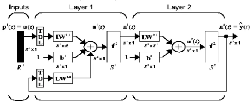
( ) ( ( )) ( ) ( ) ( ) ( ) ( )) (4) Where the dependent next value output signal y(t) is regressed on previous values of the y(t) signal and an independent (exogenous) input signal is the previous values. Implement the NARX model through feedforward neural network is to approximate the function f. A diagram of the resulting two-layer feedforward network is shown Figure 2. This application also allows for a vector ARX model for multidimensional inputs and outputs [5].

NARX network have many applications to predict the next value of the input signal and also be used for nonlinear filtering, in this a noise-free target output of the input signal will be obtained. The important use of the NARX network is established in another application of the nonlinear dynamic systems modelling. Before signifying the training of the NARX networks, vital configurations is useful in training and consider the output of the NARX network model to be prediction of the output of nonlinear dynamic system. The standard NARX architecture is output fed back to the input of the feedforward neural network.

Figure 2. Two-Layer Feedforward Network

2.1.2.1. Series parallel architecture

This architecture used when the output of the NARX network is considered to be an estimate of the output of some nonlinear dynamic system. The output is fed back to the input of the feed forward neural network as part of the standard NARX architecture. Because the true output is available during the training of the network, you could create a series-parallel architecture, in which the true output is used instead of feeding back the estimated output. This has two advantages which are the first is that the input to the feed forward network is more accurate. The second is that the resulting network has a purely feed forward architecture, and static back propagation can be used for training.

Figure 3. Series Parallel Architecture

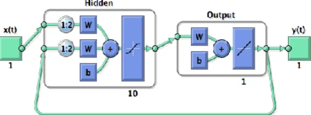
2.1.2.2. Parallel architecture

Later this architecture is converted into parallel architecture for the prediction. The prediction of the next value depends on the inputs and previous outputs to the network. The dependence on the previous output

Figure 4. Block Diagram of Parallel Architecture

2.2. Steps for train the Neural Network

Block diagram of Matlab code in Figure 5.

Figure 5. Block Diagram of Matlab Code

2.3. Algorithm of Neural Network

NARX neural network is used to solve a time series problem. [X,T] = simpleseries_dataset;

net = narxnet(1:2,1:2,10)

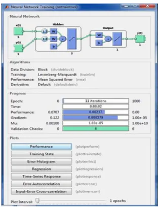
[Xs,Xi,Ai,Ts] = preparets(net,X,{},T) net = train(net,Xs,Ts,Xi,Ai);

Figure 6. Neural Network Training Diagram

View (net)

Figure 7. NARX Network View

Y = net(Xs,Xi,Ai); perf = perform(net,Ts,Y)

Here the NARX network is simulated in closed loop form. netc = closeloop(net);

[Xs,Xi,Ai,Ts] = preparets(netc,X,{},T); y = netc(Xs,Xi,Ai)

Here the NARX network is used to predict the next output a timestep ahead of when it will actually appear. netp = removedelay(net);

view(netp)

Figure 9. Prediction of Next Output of Closed Loop of NARX Network View

[Xs,Xi,Ai,Ts]=preparets(netp,X,{},T); y = netp(Xs,Xi,Ai)

3. RESULTS AND ANALYSIS 3.1. Performance of the ANN

First the collected data is preprocessed i.e. normalized and then given as inputs, which are temperatures, pressure, air density, speed and power generated is given as output to the NARX Matlab code is developed for training. After training, the neural network is ready for the prediction. The last 2 days data is given to the neural network and the predicted output is obtained. The predicted output is compared to the calculated power and the performance is monitored by calculating the errors by various means of error calculations.

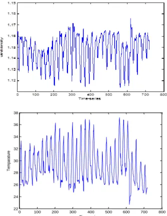
Figure 10. Collected Data Plot between air Densities, Temperatures vs Time (hours)

0 100 200 300 400 500 600 700 800

22 24 26 28 30 32 34 36 38

Time-seires

T

em

pa

ra

tu

Figure 11. Collected Data Plot between Pressures vs Time (hours)

Figure 12. Collected Data Plot between Wind Speed vs Time (hours)

a. Mean Error (ME): It is the basic type of error calculation. It is the average of the errors.

(5)

b. Mean Square Error (MSE): It is one of the basic types of error calculation. It is the average of the squares of the errors.

(6) c. Root Mean Square Error (RMSE): RMSE is the standard deviation of the differences between predicted

values and actual values. It is the square root of the average of squares of the errors.

(7) Where N - No. of samples

T-Actual Output P-Predicted Output

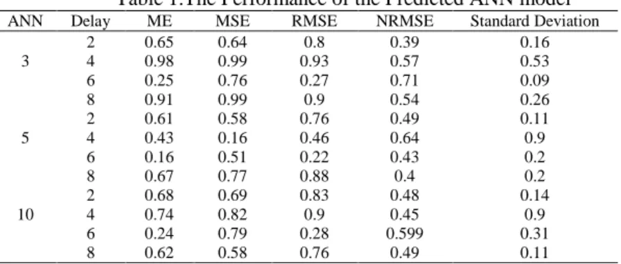
Prediction is carried out by varying the delays of the input and also the number of neurons in the hidden layer. The errors at different delays and different number of neurons in the hidden layer are

Table 1.The Performance of the Predicted ANN model

ANN Delay ME MSE RMSE NRMSE Standard Deviation

3

2 0.65 0.64 0.8 0.39 0.16

4 0.98 0.99 0.93 0.57 0.53

6 0.25 0.76 0.27 0.71 0.09

8 0.91 0.99 0.9 0.54 0.26

5

2 0.61 0.58 0.76 0.49 0.11

4 0.43 0.16 0.46 0.64 0.9

6 0.16 0.51 0.22 0.43 0.2

8 0.67 0.77 0.88 0.4 0.2

10

2 0.68 0.69 0.83 0.48 0.14

4 0.74 0.82 0.9 0.45 0.9

6 0.24 0.79 0.28 0.599 0.31

8 0.62 0.58 0.76 0.49 0.11

0 100 200 300 400 500 600 700 800

294 296 298 300 302 304 306 308 310 312

Time in hours

w in d p re s s u re

0 100 200 300 400 500 600 700 800

0 0.5 1 1.5 2 2.5 3 3.5 4 4.5 W in d s p e e d i n m /s e c Time- series

3.2. Performance Plots of the ANN

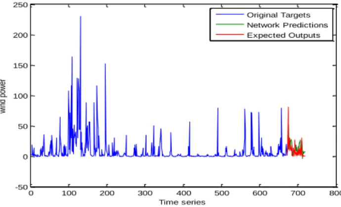
The trained neural network Levenberg-Marquardt (trainlm) is employed for the prediction of the power generated for the last 48 days by giving the input parameters by varying the input time delays and also changing the number of neurons in the hidden layer. In case of 3 neurons in the hidden layer the minimum error is attained when the time delay given is 8 and in case of 5 neurons in the hidden layer the minimum error are attained when the delay given is 6 are shown.

Figure 13. The ANN predicted output plot when 3 hidden layer neurons and time delay of 8

Figure 14. The ANN Predicted Output Plot when 5 Hidden Layer Neurons with Time Delay of 6

For short term prediction of wind power persistence method seems to be the bench mark, but by considering wind direction and upon proper training of the network the ANN model becomes more reliable according to the research and results are present in [6]. And as the time period increases the efficiency of the method decreases drastically, but the model presented in this paper can adopt itself to the varied time(s) upon successful training. The model is less complex, doesn’t contain any filters, which makes it cheaper in realization of the model but with approximately same efficiencies when compared to the other models such as Bayesian approach, Mycielski, fuzzy logic, grey model and etc.[11]-[12].

4. CONCLUSION

This paper addresses the problem a wind power forecasting model with the help of artificial neural networks (ANN). It is developed so that the wind power can be forecasted an hour before, which helps in maintaining grid interconnection and also scheduling of units. This paper not only compares the different layers and delays but also provides comparative analysis of different models. Among the different methods, the proposed is more reliable for any type of prediction and cheapest solution. Of all, the model with hidden layer size 3 and delay 6 and also the model with hidden layer size 5 and delay 6 have shown best performance among all the combinations.

0 100 200 300 400 500 600 700 800

-50 0 50 100 150 200 250

Time series

w

in

d

po

w

er

Original Targets Network Predictions Expected Outputs

0 100 200 300 400 500 600 700 800

-50 0 50 100 150 200 250

Time series

w

in

d

po

w

er

Original Targets Network Predictions Expected Outputs

REFERENCES

[1] Zhao, X Wang, SX Li, T. Review of evaluation criteria and main methods of wind power forecasting. Energy Procedia. 2011; 12: 761–769.

[2] Jaesung Jung, Robert P Broadwater. Current status and future advances for wind speed and power forecasting.

Renewable and Sustainable Energy Reviews. 2014; 31: 762-777.

[3] Yao Zhang, Jianxue Wang, Xifan Wang. Review on probabilistic forecasting of wind power generation. Renewable and Sustainable Energy Reviews. 2014; 32: 255-270.

[4] A Tascikaraoglu, M Uzunoglu. A review of combined approaches for prediction of short-term wind speed and power. Renewable and Sustainable Energy Review. 2014; 34: 243-254.

[5] Bhaskar K, Singh SN. AWNN-Assisted Wind Power Forecasting Using Feed-Forward Neural Network. IEEE Transactions on Sustainable Energy. 2012; 3: 306-315.

[6] Wen-Yeau Chang. Short-Term Wind Power Forecasting Using the Enhanced Particle Swarm Optimization Based Hybrid Method. Energies. 2013; 6: 4879-4896.

[7] Catalão, JPS Osório, GJ Pousinho, HMI. Short-Term Wind Power Forecasting Using a Hybrid Evolutionary Intelligent Approach. In Proceedings of the 16th International Conference on Intelligent System Application to Power Systems (ISAP), Hersonissos, Greece. 2011; 25: 1–5.

[8] Pan Zhao, Jiangfeng Wang, Junrong Xia, Yingxin Sheng, Jie Yue. Performance evalution and accuracy enhancement of a day-ahead wind power forecasting in china. Renewable Energy. 2012; 43: 234-241.

[9] M Carolin Mabel, E Fernandez. Analysis of wind power generation and prediction using ANN: A case study.

Renewable Energy. 2008; 33: 986-992.

[10] H Liu, HQ Tian, C Chen, Y Li. A hybrid statistical method to predict wind speed and wind power. Renewable Energy. 2010; 35: 1857-1861.

[11] IJ Ramirez-Rosado, LA Fernandez-Jimenez, C Monteiro, J Sousa, R Bessa. Comparison of two new short-term wind- power forecasting systems. Renewable Energy. 2009; 34: 1848-1854.

[12] P Flores, A Tapia, G Tapia. Application of a control algorithm for wind speed prediction and active power generation. Renewable Energy 2005; 30: 523-536.

[13] FO Hocaoglu, M Fidan, O. Gerek. Mycielski approach for wind speed prediction. Energy Conversion and Management. 2009; 50: 1436-1443.

[14] M Monfared, H Rastegar, HM Kojabadi. A new strategy for wind speed forecasting using artificial intelligent methods. Renewable Energy. 2009; 34: 845-848.

[15] M Nandana Jyothi, V Dinakar. Short-term Wind Speed Forecasting through ANN. International Journal of Applied Engineering Research. 2015; 10; 21475-21486.