Sharif University of Technology
Scientia IranicaTransactions E: Industrial Engineering www.scientiairanica.com
A compromise decision-making model based on VIKOR
for multi-objective large-scale nonlinear programming
problems with a block angular structure under
uncertainty
B. Vahdani
a;, M. Salimi
aand S.M. Mousavi
ba. Faculty of Industrial and Mechanical Engineering, Qazvin Branch, Islamic Azad University, Qazvin, P.O. Box 3419759811, Iran. b. Department of Industrial Engineering, College of Engineering, University of Tehran, Tehran, P.O. Box 18151-159, Iran. Received 6 August 2013; received in revised form 7 July 2014; accepted 1 November 2014
KEYWORDS VlseKriterijumska-Optimizacija I Kompromisno Resenje (VIKOR);
Multiple Criteria Decision Making (MCDM); Multi-Objective Decision Making (MODM); Multi-Objective Large-Scale Nonlinear Programming
(MOLSNLP); Block angular structure.
Abstract. This paper proposes a model on the basis of VlseKriterijumska Optimizacija I Kompromisno Resenje (VIKOR) methodology as a compromised method to solve the Multi-Objective Large-Scale Nonlinear Programming (MOLSNLP) problems with block angular structure involving fuzzy coecients. The proposed method is introduced for solving large scale nonlinear programming in fuzzy environment for rst time. The problem involves fuzzy coecients in both objective functions and constraints. In this method, an aggregating function developed from LP- metric is based on the particular measure of \closeness" to the \ideal" solution. The solution process is composed of two steps: First, the decomposition algorithm is utilized to reduce the q-dimensional objective space into a one-dimensional space. Then a multi-objective identical crisp non-linear programming is derived from each fuzzy non-linear model for solving the problem. Second, for nding the nal solution, a single-objective large-scale nonlinear programming problem is solved. In order to justify the proposed method, an illustrative example is presented and followed by description of the sensitivity analysis.
© 2015 Sharif University of Technology. All rights reserved.
1. Introduction
Decision making is the processes by which a course of action is selected from among several alternatives on the basis of multiple criteria. Many decision-making problems in management and engineering involve mul-tiple requirements which reect technical and eco-nomical performance in selecting the course of action while which satises both environment and resources constraints. In other words, there are many decision
*. Corresponding author. Mobile: +98 9122878561; E-mail address: [email protected] (B. Vahdani)
problems with multiple objectives in a decision-making process [1-3]. The complexity of many real situation problems increases when the number of variables is very large. In other words there are various factors in the objective functions and constraints in such problems. Specially, the computational complexity in-creases sharply in nonlinear objectives and constraints with large variables. Therefore it becomes dicult to obtain ecient solutions for these problems in a short time and ecient manner. However, most of the real-world large scale programming problems of practical interest usually has some special structures that can be exploited. Block angular structure is one of such
familiar structures [1,4-6]. The block angular structure problems are solved by a decomposition method [4].A decomposing algorithm is introduced for parametric space in large scale linear optimization problems with fuzzy parameter [4,7].Then this method is applied on large-scale nonlinear programming problems with block angular structure [6,8].
Recently, some compromise Multi-Criteria Deci-sion-Making (MCDM) methods are extended and ap-plied to nd the suitable solution for MOLSNLP problems. TOPSIS method is utilized for solving multi-objective dynamics programming problems [9,10]. An eective approach is present based on TOPSIS for solving the inter-company comparison process prob-lem [11]. TOPSIS is extended for solving multi-person multi-criteria decision-making problems in fuzzy envi-ronment [12]. An extended TOPSIS method is also presented for solving MODM problems [13]. TOPSIS is extended to solve MOLSNLP problems with block angular structure [1].
VIKOR is another compromise MCDM method that is extended for solving MOLSNLP prob-lems [5,14,15]. The VIKOR method was proposed as a compromised approach to prioritize and select from among a set of alternatives on the basis of conicting or non-commensurable criteria. The VIKOR is uti-lized to nd suitable solution based on the particular measure of closeness to the ideal solution [14,15]. The VIKOR method was extended in 2007 [16-18]. This method is employed for making decision about eective information technology outsourcing management in a real-time decision situation [19]. Moreover, a system-atic procedure is developed using MCDM compromise ranking method VIKOR to optimize the multi-response process [20]. The VIKOR method is also extended to prioritize alternatives with fuzzy parameter by many researchers. The fuzzy sets and VIKOR method is integrated to fuzzy VIKOR for solving the fuzzy MCDM programming problems [21]. Thus VIKOR is an interactive method in developing methods and its applications. Although, a large body of studies has uti-lized crisp and exact data, uncertainty and vagueness are the prominent characteristic of many real world situation decision making problems. In other words it is obvious that much knowledge in the real world is uncertain rather than crisp [22,23]. Fuzzy set theory is a valuable tool for describing this concept. Fuzzy set theory was proposed as a vagueness concept for decision-making problems with conict of preferences involved in the selection process [22,24]. Moreover, the fuzzy set concept and the MCDM method were manipulated to consider the fuzziness in the decision making parameter and group decision-making process. A fuzzy MCDM process was introduced based on the fuzzy model and concepts of positive and neg-ative ideal points for solving MCDM problems in
a fuzzy environment [25,26].The studies also focused on applying MCDM methods for solving MOLSNLP problems with crisp parameters in objective functions and constrain [1]. The VIKOR method is utilized for solving MOLSNLP problems where the formulation of objective functions and constraints is introduced with crisp data whereas coecient of objective function and constraint may not be exact and complete. Moreover, Abo-Sinna and Abou-El-Enien proposed a TOPSIS in-teractive algorithm to solve large scale multi-objective programming problems with fuzzy parameters and only for linear programming problems [27].
In this paper, a new extended VIKOR is proposed for solving MOLSNLP problems with block angular structure where the problem is formulated with fuzzy parameters in the objective functions and constraints. Since in real situations, the information of decision maker related to coecient of objective function and constraint may not be exact and complete, a simple method is proposed which can be applied to formulate the equivalent crisp model of the fuzzy optimization problem. Moreover, the proposed method is utilized for solving nonlinear problems with fuzzy parameters, whereas the recent research studies focus only on the linear programming problems with fuzzy parameters. In the present study, rst, the decomposition algorithm is used to reduce the q-dimensional objective space into a one-dimensional space. Then a multi-objective identical crisp non-linear programming is derived from each fuzzy non-linear model for solving the problem. Second, a model with fuzzy coecients in objective function will be transferred to crisp model. Then, the method is applied for fuzzy constraints. Fol-lowing that, a single-objective The logic of VIKOR method is utilized to aggregate the multi-objective programming problems into single-objective. In sum, it transfers n objectives, which are conicting, into single-objectives involving the maximum \group util-ity" for the \majorutil-ity" and a minimum of an individual regret for the \opponent", based on the shortest distance from the PIS and the longest distance from the NIS, which are commensurable and most of time conicting. Following that, a single-objective large-scale nonlinear programming problem is solved to nd the nal solution. Finally, the Sensitivity analysis is described.
The remainder of this paper is organized as follows. The problem formulation is presented in the next section. In this section, the decomposed problem is introduced and then the parameters and variables are described. In Section 3, the VIKOR Solution method for fuzzy MOLSNLP is introduced. In Section 4, an example is provided to illustrate the process of proposed method step by step. Then, the Sensitivity analysis is described for each sub-problem. The last section is devoted to conclusion.
2. Problem formulation
The large-scale problems represent major companies that are composed of multiple units. The sub systems are almost independent with respect to each other. In other words the objective functions can be decomposed into some objectives.
A fuzzy MOLSNLP problem with the block an-gular structure can be stated as follows:
p :
max(min)f1(x; ~u1) = N
P
j=1f1j(xj; ~u1j)
max(min)f2(x; ~u2) = N
P
j=1f2j(xj; ~u2j)
...
max(min)fL(x; ~uL) = N
P
j=1fLj(xj; ~uLj);
s.t.:
F S = 8 > > > > > > > > > > > > > > > > > > > > > > > > < > > > > > > > > > > > > > > > > > > > > > > > > :
~gm(x1) ~B1
m = 1; 2; ; s1
~gm(x2) ~B2
m = s1; 2; ; s2
...
~gm(xN) ~BN
m = sr+1; 2; ; sM
~ Hi(x) =
N
P
j=1~hij(xj) ~B
i = 1; 2; ; w
(1)
fi(x; ~ui)= ~uicix= N
X
j=1
fij(xj; ~ui)= N
X
j=1 p
X
k=1
~uijkcijkvijk(x);
(2) where Vijk(Xj) is the kth function of jth variable in
the ith objective function. This problem is a fuzzy MOLSNLP problem with the block angular structure as a big company which has q sub system. Moreover, there are N variables. Each sub problem has its own variables. For example the rst sub problem has N1
variables. Furthermore, the functions of each sub problem has several functions.
~gi(xj) = ~uijcijvij are the inequality constraint
functions and ~Hi(x) are the common constraint
func-tions on Rn.
Model parameters:
L The number of objective functions; q The number of sub problems;
N The number of variables;
Ni The set of variables of the ith sub
problem, i = 1; 2; ; q; pi ith sub problems;
pitj The number of functions for tth
function of jth variable in ith sub problem;
R The set of all real numbers;
ci An (N N) diagonal matrix for the
ith function;
citj An (N N) diagonal matrix for the
kth function of the jth variable in the ith function;
cij An (N N) diagonal matrix for the
ith constraint of jth variable; dij An (N N) diagonal matrix for the
ith common constraint for the jth variable;
~
Ui An n-dimensional row vector of fuzzy
parameters for the ith objective function;
~
Uij An n-dimensional row vector of fuzzy
parameters for the ith constraint of jth variable;
~
Uijk An n-dimensional row vector of fuzzy
parameters for the kth function of the jth variable in the ith function; W The number of common constraints on
RN;
M The number of constraints;
Si the number of constraints for the ith
variable; ~
B An w-dimensional column vector of right-hand sides of the common constraints whose elements are constants;
~
Bj An Si-dimensional column vector of
independent constraints right-hand sides whose elements are fuzzy parameters for the ith subproblem, i = 1; 2; ; q.
X = (x1; x2; ; xN) is the N-dimensional decision
vector. fi(x; ~ui), i = 1; 2; ; L are the objective
functions. It is assumed that the objective functions have an additively separable form. It is pointed out that any (or all) of the functions may be nonlinear. The fuzzy MOLSNLP problem can be decomposed into q sub-problems based on Dantzig-Wolfe decomposition algorithm. The objective functions break into q sub problems. The ith sub-problem for i = 1; ; q is
dened as:
Pi=
8 > > > > > > > > > > > > > > > > > > > > > > > > > > > > > > > > > > > > > > > > > > > > > > < > > > > > > > > > > > > > > > > > > > > > > > > > > > > > > > > > > > > > > > > > > > > > > :
max(min)f1(x; ~u1) =
X
j2Ni
pi1j
X
k=1
f1k(xj; ~u1k)
= X
j2Ni
pi1j
X
k=1
~u1kc1kv1k(xj)
max(min)f2(x; ~u2) =
X
j2Ni
pi2j
X
k=1
f1k(xj; ~u2k)
= X
j2Ni
pi2j
X
k=2
~u2kc2kv2k(xj)
...
max(min)fL(x; ~uL) =
X
j2Ni
pXiLj
k=1
fLk(xj; ~uLk)
= X
j2Ni
pXiLj
k=1
~uLkcLkvLk(xj)
S:T: F Si=
8 > > > > < > > > > : P j2Ni
~gj(xj) ~Bj
~ Hi(x) =
N
P
j=1~hij(xj) ~B
i = 1; 2; ; w
(3)
As shown in Problem (3), the ith sub problem consists of L objective functions. There are Pitj functions
for jth variable of tth objective function in ith sub problem. Moreover, ~hij(Xj) = ~Uijdijhij, where hij is
the function of jth variable in ith common constraint and ~U is the coecient of the objective function, ~C and ~Z are the coecients of the left-hand side of constraints, and ~B is the coecient of the right-hand side of constraint in Problem (3). It is pointed out that all of the coecients are presented as triangular fuzzy numbers.
3. The VIKOR solution method for fuzzy MOLSNLP
In this section, a compromised method based on VIKOR is presented for solving fuzzy MOLSNLP problems. The basic methodology is to decompose the original problem into smaller sub-problems. In other words this method is employed when the original problem is split into some sub-problems. In order to obtain a compromise solution, rst, the MOLSNLP problem is decomposed into q sub-problems as shown in Eq. (3). Then by considering the individual minimum and maximum of each objective function, the Positive Ideal Solution (PIS) and Negative Ideal Solution (NIS) for jth sub-problem are computed. By Computing
Sj; Rj; Qj, the L-dimensional problem is transferred
into a single-objective. The proposed method is administered through the following steps:
Step 1. Decompose the proposed problem into the q sub-problems based on the Dantzig-Wolfe decomposi-tion algorithm for objective funcdecomposi-tions and constraints. Then transfer each fuzzy sub problem into three crisp sub problems as follows:
~
Ui= (ai;bi;ci);
is a triangular fuzzy number. fi(x; ~ui) = ~uicix =
N X j=1 pi X k=1
~uijkcijkvijk(xj)
=XN
j=1 pi
X
k=1
(aijk;bijk;cijk)cijkvijk(xj); (4)
i = 1; 2; ; L;
Pi=
8 > > > > > > > > > > > > > > > > > > > > > > > > > > > > > > > > > > > > > > > > > > < > > > > > > > > > > > > > > > > > > > > > > > > > > > > > > > > > > > > > > > > > > :
max(min)f1(x; ~u1) =
X
j2Ni
pi1j
X
k=1
(aijk;bijk;cijk)cijkvijk(xj)
max(min)f2(x; ~u2) =
X
j2Ni
pi2j
X
k=1
(aijk;bijk;cijk)cijkvijk(xj)
...
max(min)fL(x; ~uL) =
X
j2Ni
piLj
X
k=1
(aijk;bijk;cijk)cijkvijk(xj)
S.T:
F Si=
8 > > > > > > > > > < > > > > > > > > > : P j2Ni
~gj(xj) ~Bj
m = sj 1+ 1; ; sj
~ Hi(x) =
N
P
j=1~hij(xj) ~B
i = 1; 2; ; w
(5)
s.t. (x1; x2; ; xN) 2 F S:
The sub problems can be solved independently and their solution could be used to compute Sj; Rj; Qj.
So, using a simple approach which is adopted by some researchers [28-30], each fuzzy problem is converted to three crisp problems. In other words, we introduce three crisp sub problems (Pij) instead of each fuzzy
sub problem (Pi) as follows:
Pi1:
8 > > > > > < > > > > > :
min(max)(b1 a1)(c1v1(xj))
min(max)(b2 a2)(c2v2(xj))
...
min(max)(bL aL)(cLvL(xj))
(6)
Pi2:
8 > > > > > < > > > > > :
max(min)b1(c1v1(xj))
max(min)b2(c2v2(xj))
...
max(min)bL(cLvL(xj))
(7)
Pi3:
8 > > > > > < > > > > > :
max(min)(c1 b1)(c1v1(xj))
max(min)(c2 b2)(c2v2(xj))
...
max(min)(cL bL)(cLvL(xj))
(8)
Moreover, transfer each fuzzy constraint into three crisp constraints as follow:
We can consider the fuzzy constraint as bellow: ~gm(xj) ~Bm; m = sj 1+ 1; ; sj;
j = 1; 2; ; N;
~gm(xj) = ~cmgi(xj) = (cm1; cm2; cm3)gm(xj);
~cm= (cm1; cm2; cm3);
~bm= (cm1; cm2; cm3);
8 > > > < > > > :
~cm1gm(xj) ~bm1
~cm2gm(xj) ~bm2
~cm3gm(xj) ~bm3
(9)
where ~cm is fuzzy coecient of objective function and
~
Bm is fuzzy coecient of constraints.
~ Hi(x) =
N
X
j=1
~hij(xj) ~B; (10)
~hij(xj) = ~zij(xj)hij(xj); (11)
~ Hi(x) =
N
X
j=1
~zij(xj)hij(xj) ~B; (12)
~
zij = (zij1; zij2; zij3); (13)
~
B = (rij; sij; tij); (14)
N
X
j=1
zij1hij(xj) ri; N
X
j=1
zij2hij(xj) si;
N
X
j=1
zij3hij(xj) ti;
i = 1; 2; :::; w j = 1; 2; ; N: (15) Therefore, the constraints of sub problem (Pi) are
transferred to the following form: 8 > > > > > > > > > > > > > > > > > > > > > > > > > > > > > > > > < > > > > > > > > > > > > > > > > > > > > > > > > > > > > > > > > : 8 > < > :
r11gm(x1) b11
r12gm(x1) b12 m = 1 ; s1
r13gm(x1) b13
8 > < > :
r21gm(x2) b21
r22gm(x2) b22 m = s1+ 1; ; s2
r23gm(x2) b23
... 8 > < > :
rq1gm(xq) bq1
rq2gm(xq) bq2 m = sr+ 1; ; sM
rq3gm(xq) bq3 N
P
j=1zi1hij(xj) ri N
P
j=1zi2hij(xj) si i = 1; 2; ; w N
P
j=1zi3hij(xj) ti
(16)
Step 2. Using VIKOR approach, rst calculate the maximum f
ijvalue as Positive Ideal Solution (PIS) and
the minimum ~fij value as Negative Ideal Solution (NIS) of each objective function under the given constraints for variable xj. The benet and cost objectives are
indexed as: f
bj = fmax(min)fbj(xj)(fcj(xj)); 8 b(8 c)g;
fbj = fmin(max)fbj(xj)(fcj(xj)); 8 b(8 c)g; (17)
fbj(xj) Benet objective for maximization,
fcj(xj) Cost objective for maximization.
Then Compute the amount of Sj, Rj and Qj as
follows: Sj =
X
b2B
wb f
bj fbj(Xj)
f bj fbj
!
+X
c2B
wc fcj(Xj) f cj
fcj f cj
!
Rj= max
( wb f
bj fbj(xj)
f bj fbj
! ;
wc fbj(xj) f bj
fbj f bj
!)
; (19)
min s.t. wb f
bj fbj(xj)
f bj fbj
! ; wc fbj(xj) f
bj
fbj f bj
!
; (20)
s
j = min(sj); sj = max(sj);
R
j = min(Rj); Rj = max(Rj); (21)
Qj = sj s j
sj s j
!
+ (1 ) Rj Rj Rj R j
!
; (22) where, Wb(Wc) represents weights of objective
func-tions, Sj represents the distance of the jth objective
function achievement to the positive ideal solution, and Rj implies maximal regret of each objective function,
and is a weight of the strategy for Sj and Rj. In
other word, the decision making strategy can be used with maximum group utility ( > 0:5), with consensus ( = 0:5), or with minimum individual regret ( < 0:5) (Vahdani et al., 2010; Opricovic, 1998).
Step 3. From the results of Step 2, determine the constraints corresponding to the each Qij. Afterward
construct the nal single-objective problem according to the values of Qij, for each problem as will be shown
in Eq. (30). Then solve it to obtain the nal optimal solution.
min 1+ 2+ + q;
s.t. Q11 1
Q12 1
Q13 1
...
Qq1 q
Qq2 q
Qq3 q
X 2 F S
(23)
Find the optimal solution vector X, where X =
(x
1; x2; ; xn) is the best value of the original MODM
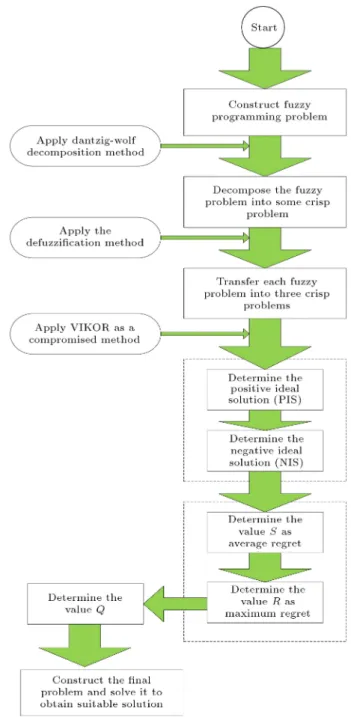
problem. Finally, the owchart of the proposed VIKOR
Figure 1. The owchart of proposed VIKOR solution method.
method for solving MOLSNLP problem is depicted in Figure 1. The proposed method is illustrated through a numerical example.
4. Illustrative numerical example
In this section, we give an example to illustrate the stages of proposed model. There are three objectives functions on R3, where the coecient of the objective
functions and constraints are proposed as triangular fuzzy numbers. It is assumed that the importance of weight is the same (w = 1=3) among the objective functions of all sub problems. The original problem
is proposed as: P :
max f1(x) =(1; 2; 3)(x1 1)2+ (2; 3; 4)x22
+ (1; 3; 5)(x3+ 1)2;
max f2(x)=(2; 4; 6)x1+(1; 2; 3)x2+(1; 3; 5)(x3)2;
min f3(x)=(1; 2; 3)(x1)2+(1; 3; 5)x2+(1; 2; 3)(x3)2;
s.t.
F S = 8 > > > > > > > > > < > > > > > > > > > :
(1; 2; 3)x1 (1; 2; 3)x2+ (2; 4; 6)x3
(6; 7; 8) (1; 2; 3)x2
1+ (1; 3; 5)x2+ (1; 2; 3)x3
(10; 11; 12) (0; 0; 0) (1; 2; 3)x1 (3; 4; 5)
(0; 0; 0) (1; 2; 3)x2 (4; 5; 6)
(0; 0; 0) (1; 2; 3)x3 (2; 3; 4)
9 > > > > > > > > > = > > > > > > > > > ; : (24)
The problem can be split into three sub-problems. Therefore the new method is exploited to obtain optimal solution in the following steps:
Step 1. In the rst stage, consider problem (P ) and decompose it into three fuzzy sub problems (P1; P2; P3). Because the coecient of the objective
functions and constraints are proposed as triangular fuzzy numbers, each objective function is transferred into three crisp functions for each fuzzy sub problem. Moreover, each fuzzy constraint is transferred to three crisp constraints. Based on the proposed method, this problem can be decomposed as the following program. First sub problem (P1) is proposed based on variable
x1.
P1:
max f1(x) = (1; 2; 3)(x1 1)2;
max f2(x) = (2; 4; 6)x1;
min f3(x) = (1; 2; 3)(x1)2;
s.t.
F S1=
8 > > > > > > > > < > > > > > > > > :
(1; 2; 3)x1 (1; 2; 3)x2+ (2; 4; 6)x3
(6; 7; 8) (1; 2; 3)x2
1+ (1; 3; 5)x2+ (1; 2; 3)x3
(10; 11; 12) (0; 0; 0) (1; 2; 3)x1 (3; 4; 5)
9 > > > > > > > > = > > > > > > > > ; : (25)
Similar to sub problem P1, sub problems P2 and P3
can be formulated as: P2:
max f1(x) = (2; 3; 4)x22;
max f2(x) = (1; 2; 3)x2;
min f3(x) = (1; 3; 5)x2;
s.t.
F S = 8 > > > > > > > > < > > > > > > > > :
(1; 2; 3)x1 (1; 2; 3)x2+ (2; 4; 6)x3
(6; 7; 8); (1; 2; 3)x2
1+ (1; 3; 5)x2+ (1; 2; 3)x3
(10; 11; 12) (0; 0; 0) (1; 2; 3)x2 (4; 5; 6)
9 > > > > > > > > = > > > > > > > > ; ; (26)
P3:
max f1(x) = (1; 3; 5)(x3+ 1)2;
max f2(x) = (1; 3; 5)(x3)2;
min f3(x) = (1; 2; 3)(x3)2;
s.t.
F S = 8 > > > > > > > > < > > > > > > > > :
(1; 2; 3)x1 (1; 2; 3)x2+ (2; 4; 6)x3
(6; 7; 8) (1; 2; 3)x2
1+ (1; 3; 5)x2+ (1; 2; 3)x3
(10; 11; 12) (0; 0; 0) (1; 2; 3)x3 (2; 3; 4)
9 > > > > > > > > = > > > > > > > > ; : (27)
Now, using Relations (6) and (20), convert each sub problem of fuzzy MONLFP (31) into its non-fuzzy version sub problem. As will be shown in Eqs. (35), (36), and (37), the sub problems P11; P12, and P13 are
constructed as: P1:
P11:
8 > > > > > > < > > > > > > :
min f1(x) = (x1 1)2
min f2(x) = 2x1
max f3(x) = (x1)2
s.t. X 2 F S1
(28)
P12:
8 > > > > > > < > > > > > > :
max f1(x) = 2(x1 1)2
max f2(x) = 4x1
min f3(x) = 2(x1)2
s.t. X 2 F S1
P13: 8 > > > > > > > > < > > > > > > > > :
max f1(x) = 2(x1 1)2
max f2(x) = 4x1
min f3(x) = 2(x1)2
s.t. X 2 F S1
(30)
The above three crisp objectives programming are equivalent to the fuzzy problem P1. Similar to P1, the
above procedure is utilized to obtain P2 as:
P2:
P21:
8 > > > > > > > > < > > > > > > > > :
min f1(x) = x22
min f2(x) = x2
max f3(x) = 2x2
s.t. X 2 F S2
(31)
P22:
8 > > > > > > > > < > > > > > > > > :
max f1(x) = 3x22
max f2(x) = 2x2
min f3(x) = 3x2
s.t. X 2 F S2
(32)
P23:
8 > > > > > > > > < > > > > > > > > :
max f1(x) = x22
max f2(x) = x2
min f3(x) = 2x2
s.t. X 2 F S2
(33)
It is clear that by Eqs. (8) and (20), the fuzzy sub problem P3 can be transferred to three crisp problem
as bellow: P3:
P31:
8 > > > > > > > > < > > > > > > > > :
min f1(x) = 2(x3+ 1)2
min f2(x) = 2(x3)2
max f3(x) = (x3)2
s.t. X 2 F S3
(34)
P32:
8 > > > > > > > > < > > > > > > > > :
max f1(x) = 3(x3+ 1)2
max f2(x) = 3(x3)2
min f3(x) = 2(x3)2
s.t. X 2 F S3
(35)
P33:
8 > > > > > > > > < > > > > > > > > :
max f1(x) = 2(x3+ 1)2
max f2(x) = 2(x3)2
min f3(x) = (x3)2
s.t. X 2 F S3
(36)
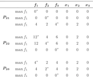
Step 2. Calculate the Positive Ideal Solution (PIS) and the Negative Ideal Solution (NIS) of each objective function for all sub problems of P1; P2, and P3as shown
in Tables 1 and 2. Next, compute the amount of Sij; Rij, and Qij for all sub problems under the given
constraints for all variables as follows: PIS : f
11= (f1; f2; f3) = (0; 0; 2:7778);
f
12= (f1; f2; f3) = (2; 6:6667; 0);
f
13= (f1; f2; f3) = (1; 3:3334; 0);
Table 1. PIS payo table of (P1).
f1 f2 f3 x1 x2 x3
P11
max f1 0 2 1 1 0 0
max f1 1 0 0 0 0 0
max f1 0.4445 3.3333 2:7778 1.6667 0 0
P12
max f1 2 0 0 0 0 0
max f1 0.8890 6:6667 5.5558 1.6667 0 0
max f1 2 0 0 0 0 0
P13
max f1 1 0 0 0 0 0
max f1 0.4445 3:3334 2.7779 1.6667 0 0
max f1 1 0 0 0 0 0
Table 2. NIS payo table of (P1).
f1 f2 f3 x1 x2 x3
P11
max f1 1 0 0 0 0 0
max f1 0.4445 3:3333 2.7779 1.6667 0 0
max f1 1 0 0 0 0 0
P12
max f1 0 4 2 1 0 0
max f1 2 0 0 0 0 0
max f1 0.8890 6.6667 5:5556 1.6667 0 0
P13
max f1 0 2 1 1 0 0
max f1 1 0 0 0 0 0
Table 3. The values of S, S , Rand R for (P 1).
PIS NIS S S R R
P11 (0,0,2.7778) (1,3.3333,0) 0.4114 0.6667 0 0.3333
P12 (2,6.6667,0) (0,0,5.5556) -0.3333 -0.0781 0 0.3333
P13 (1,3.3334,0) (0,0,2.7778) 0.3333 0.4534 0 1 NIS : f11= (f1 ; f2 ; f3) = (1; 3:3333; 0);
f12= (f1 ; f2; f3 ) = (0; 0; 5:5556); f13= (f1 ; f2; f3 ) = (0; 0; 2:7778):
The obtained PIS and NIS are shown in Table 3. Then S11 is obtained using Relation (23) as follows:
S11= 0:2133(x1)2 0:4667X1+ 0:6667: (37)
Moreover, R11is obtained using Eqs. (24) and (26) as:
min s.t.
1 3
(x1 1)2 0
1 0
; 1
3
2x1 0
3:3333 0
; 1
3
2:7778 (x1)2
2:7778 0
;
X 2 F S1; =0:2060; X=(1:030; 0; 0): (38)
The second and third constraints are active in point x = (1:030; 0; 0). Moreover, the values of R; R for
both constraints are the same. Therefore, each of the second and third constraints can be chosen anyas R11.
Here we choose the second constraint, so simplied R11
is as follows:
R11= 0:2x1: (39)
Suppose that the compromise is selected with \consen-sus" ( = 0:5). Then Q11 is obtained by computing
Relation (29).The simplied result is as follows: Q11= 0:4177x21 0:6140X1+ 0:5: (40)
Similar to P11, the values of S, R, and Q are obtained
for problems P12and P13, as follow:
S12= 0:2133x21+ 0:4666X1 0:3333; (41)
R12= 0:3333x21+ 0:6666X1; (42)
Q12= 0:9179x21+ 1:9142X1; (43)
S13= 0:4533x21+ 0:4666X1+ 0:3333; (44)
R13= 0:3333x21+ 0:6666X1; (45)
Q13= 2:0539x21+ 0:05667X1: (46)
The amounts of S; S ; R, and R are obtained for
problems P11; P12, and P13, as shown in Table 3, where:
S
ij(Sij) = max(min Sij);
R
ij(Rij) = max(min Rij);
s.t. X 2 F Si:
Similar to P1, the values of PIS and NIS of each
objective function for all sub problems of P2 are
calculated in Tables 4 and 5.
Table 4. PIS payo table of (P2).
f1 f2 f3 x1 x2 x3
P21
max f1 0 0 0 0 0 0
max f1 0 0 0 0 0 0
max f1 4 2 4 0 2 0
P22
max f1 12 4 6 0 2 0
max f1 12 4 6 0 2 0
max f1 0 0 0 0 0 0
P23
max f1 4 2 4 0 2 0
max f1 4 2 4 0 2 0
max f1 0 0 0 0 0 0
Table 5. NIS payo table of (P2).
f1 f2 f3 x1 x2 x3
P21
max f1 4 2 4 0 2 0
max f1 4 2 4 0 2 0
max f1 0 0 0 0 0 0
P22
max f1 0 0 0 0 0 0
max f1 0 0 0 0 0 0
max f1 12 4 6 0 2 0
P23
max f1 0 0 0 0 0 0
max f1 0 0 0 0 0 0
Table 6. The values of S, S , Rand R for (P 2).
PIS NIS S S R R
P21 (0,0,4) (4,2,0) 0.3333 0.6665 0 0.3333
P22 (12,4,0) (0,0,6) 0.3335 0.6667 0.2060 0.3333
P23 (4,2,0) (0,0,4) 0.3335 0.6667 0.2060 0.3333 The values of PIS and NIS are shown in Table 6. The values of S, R, and Q are obtained for problems P2 as follow.
First, the values of S21and R21are obtained as:
S21= 0:0833x22+ 0:3333; (47)
min ; s.t. 1 3
(x2)2
4 0
; 1
3
x2
2 0
; 1
3
4 2x2
4 0
; X 2 F S2;
=0:1667; X=(1; 0; 0); R
21=0:1667X2: (48)
The simplied result of Q21 is as follow:
Q21= 0:375X22 0:5002: (49)
Similar to sub problem P21, S, S , R and R are
obtained for problems P22 and P23. The values of S22
and R22 are obtained similar to privies steps as:
S22= 0:0833X22+ 0:6667; (50)
R22= 0:6667X2: (51)
The value of Q22 is calculated as:
Q22= 0:125X22+ 0:6546X2 0:3091: (52)
In last step for sub problem P2, the values of S23 and
R23 are calculated as:
S23= 0:0833X22+ 0:6667; (53)
R23= 0:6667X2; (54)
Q23= 0:125X22+ 0:6546X2 0:3091: (55)
S, S , R, and R are obtained for problems P 21,
P22, and P23as shown in Table 6.
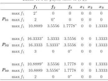
Table 7. PIS payo table of (P3).
f1 f2 f3 x1 x2 x3
P31
max f1 2 0 0 0 0 0
max f1 2 0 0 0 0 0
max f1 10.8889 3.5556 1:7778 0 0 1.3333
P32
max f1 16:3333 5.3333 3.5556 0 0 1.3333
max f1 16.3333 5:3333 3.5556 0 0 1.3333
max f1 3 0 0 0 0 0
P33
max f1 10:8889 3.5556 1.7778 0 0 1.3333
max f1 10.8889 3:5556 1.7778 0 0 1.3333
max f1 2 0 0 0 0 0
Table 8. NIS payo table of (P3).
f1 f2 f3 x1 x2 x3
P31
max f1 10:8889 3.5556 1.7778 0 0 1.3333
max f1 10.8889 3:5556 1.7778 0 0 1.3333
max f1 2 0 0 0 0 0
P32
max f1 3 0 0 0 0 0
max f1 3 0 0 0 0 0
max f1 16.3333 5.3333 3:5556 0 0 1.3333
P33
max f1 0 0 0 0 0 2
max f1 0 0 0 0 0 2
max f1 3.5556 1:7778 0 0 1.3333 10.8889 Consequently, the values of PIS and NIS of each objective function for all sub problems of P3 are
calculated in Tables 7 and 8.
The values of PIS and NIS are shown in Tables 7 and 8.
S31= 0:075X32+ 0:075X3+ 0:3333; (56)
min ; s.t.
1 3
2(x3+ 1)2 2
10:8889 2
; 1
3
2x2 3 0
3:5556 0
; 1
3
1:7778 (x3)2
1:7778 0
; X 2 F S2;
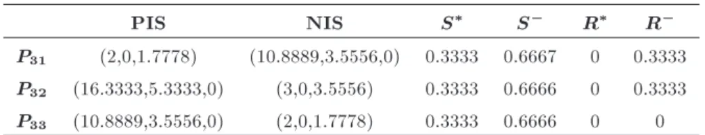
Table 9. The values of S, S , Rand R for (P 3).
PIS NIS S S R R
P31 (2,0,1.7778) (10.8889,3.5556,0) 0.3333 0.6667 0 0.3333
P32 (16.3333,5.3333,0) (3,0,3.5556) 0.3333 0.6666 0 0.3333
P33 (10.8889,3.5556,0) (2,0,1.7778) 0.3333 0.6666 0 0 R31= 0:0375X32+ 0:075X3: (58)
Similar to sub problem P21, S, S , R, and R are
obtained for problems P22and P23, as shown in Table 9.
Q31= 0:15X32+ 0:3X3: (59)
Also similar to sub problem P31, the values for S32,
R32, and Q32 are obtained as:
S32= 0:075X32 0:15X3+ 0:6667; (60)
R32= 0:1875X32; (61)
Q32= 0:0:3938X32 0:2250X3+ 0:5: (62)
In last step for sub problem P3, the values of S33, R33,
and Q33 are calculated as:
S33= 0:075X32 0:15X3+ 0:6667; (63)
R33= 0:1875x23; (64)
Q33= 0:1688X32 0:2250X3+ 0:5: (65)
S, S , R, and R are obtained for problems P 31,
P32, and P33 as shown in Table 9.
Step 3. From the results of Step 2 determine the constraints corresponding to the each Qij. Afterward
construct the nal single-objective problem according to the values of Qij for each problems shown in
Eq. (74). Then solve it to obtain the nal optimal solution. The crisp single-objective problem for the numerical example is as follows:
min 1 + 2 + 3; 0:4177x2
1 0:6140x1+ 0:5 1;
0:9179x2
1+ 1:9142x1 1;
2:0539x2
1+ 0:5667x1 1;
0:375x2
2 0:5002x2 2;
0:125x2
2+ 0:6546x2 0:3091 2;
0:0833x2
2+ 0:6667 2;
0:15x2
3+ 0:3x3+ 0:5 3;
0:3938x2
3 0:2250x3 3;
0:1688x2
3 0:2250x3 3;
x2
1 x2+ 2x3 6; 2x1 2x2+ 4x3 7;
3x1 3x2+ 6x3 8; x21+ x2+ x3 10;
2x2
1+ 3x2+ 2x3 11; 3x21+ 5x2+ 3x3 12;
0x13; 02x14; 03x15;
0x24; 02x25; 03x26;
0x32; 02x33; 03x34: (66)
Find the optimal solution vector X, where X =
(x
1; x2; ; xn) is the best value of the original MODM
problem. By solving Problem (74), we obtain the optimum minimum value of 1, 2, and 3, as follows:
z= 0:4679; X= (0:2244; 1:5957; 0:2857);
1= 0:3833; 2= 0:4546; 3= 0:2857:
4.1. Sensitivity analysis
In this example, as it was observed, there are three objectives on R3. Moreover, the optimal solution
vector X = (x
1; x2; ; xn) where x1, x2, and x3
are obtained from sub problems P1, P2, and P3,
respectively. Considering Problem (74), the inequality constraint is proposed in three categories. First group of them are constructed based on the Q11, Q12, and
Q13 where Qij is applied as functions of the left-hand
side of the inequality constraints. The amount of
1 is determined according to objective function and
constraints. When x1increases from 0.2244, the values
of functions Q12and Q13will be decreased but the rst
inequality is impossible because the amount of Q11 is
more than right-hand side of constraint. Therefore, simultaneously according to the objective function and constraint, x1 = 0:2244, is optimal solution for x1.
Figure 2 represents the behavior of Q11, Q12, and Q13
based on x1.
Similar to P1, the problems P2and P3 are solved.
Figure 2. The values of function Qij for problem P1.
Figure 3. The values of function Qij for problem P2.
Figure 4. The values of function Qij for problem P3. Q22 and Q23 will be decreased but the amount of
Q21 is more than right-hand side of rst constraint.
Moreover, When x2decreases from 1.5957 the amount
of Q21 will be decreased but the values of functions
Q22 and Q23 is more than right-hand side of rst and
second constraints, respectively, as shown in Figure 3. Therefore, x2 = 1:5957 is the best solution of problem
P2.
Also similar to the problems P1 and P2, the
optimal solution of P3 is x3 = 0:2857, as shown in
Figure 4. 5. Conclusion
In this paper, the focus was on extending and applying a VIKOR approach as a compromise decision making method to deal with MOLSNLP problems with block
angular structure under uncertainty. The proposed method was introduced for solving large scale nonlinear programming in fuzzy environment for rst time. The new method employed the advantages of VIKOR as a compromised method for solving nonlinear prob-lems. First, Dantzig-Wolfe decomposing algorithm was applied to decompose the n-dimensional space fuzzy MOLSNLP into n sub problems. In the proposed approach, the sub problems in fuzzy environment were solved by converting them into crisp environment. In other words, each fuzzy problem can lead to three crisp problems. Then the proposed VIKOR method was applied to obtain an equation for each sub problem in a crisp single-objective problem. Therefore, it can be argued that this method combines LSMONLP and VIKOR approach to obtain a compromise solution of the problem. In sum, it transfers n objectives, which are conicting, into single-objectives involving the maximum \group utility" for the \majority" and a min-imum of an individual regret for the \opponent", based on the shortest distance from the PIS and the longest distance from the NIS, which are commensurable and most of time conicting. In other words, the VIKOR has been applied in MADM for ranking the alternatives versus some criteria whereas this paper applied VIKOR in MODM problems. The logic of VIKOR method was utilized to aggregate the multi-objective programming problems into single-objective. The MODM problems were considered with fuzzy parameters in objective function and constraints. Moreover, the constraints could be considered as non-linear equation. Finally, to justify the proposed method, an illustrative example was provided. The numerical example has three sub problems. The new method is utilized to solve each problem. The optimum solution and satisfaction value of each sub problem was proposed in sensitivity analysis. The optimum value of objective function is Z = 0:4679. Moreover the amounts of variables
are x = (0:2244; 1:5957; 0:2857) and the satisfaction
values of each sub problem are
1 = 0:3833, 2 =
0:4546, and
3 = 0:2857. For the future research, an
MCDM method can be presented with interval data for solving the multi-objective nonlinear programming problems in large scale context.
References
1. Abo-Sinna, M.A. and Amer, A.H. \Extensions of TOPSIS for multi-objective large-scale nonlinear pro-gramming problems", Applied Mathematics and Com-putation, 162, pp. 243-256 (2005).
2. Hu, C., Shen, Y. and Li, S. \An interactive satiscing method based on alternative tolerance for fuzzy mul-tiple objective optimization", Applied Mathematical Modelling, 33, pp. 1886-189 (2009).
S.M.H \A multi-criteria decision-making approach with interval numbers for evaluating project risk re-sponses", IJE Transactions B: Applications, 25(2), pp. 121-130 (2012).
4. Dantzig, G. and Wolfe, P. \The decomposition algo-rithm for linear programming", Econometrica, 29, pp. 767-778 (1961).
5. Sakawa, M., Large Scale Interactive Fuzzy Multi-Objective Programming, Physica-Verlag, Springer-Verlag Company, New York (2000).
6. Heydari, M., Sayadi, M.K. and Shahanaghi, K. \Ex-tended VIKOR as a new method for solving multi-ple objective large-scale nonlinear programming prob-lems", RAIRO Operations Research, 44, pp. 139-152 (2010).
7. El-Sawy, A.A., El-Khouly, N.A. and Abou-El-Enien, T.H.M. \An algorithm for decomposing the parametric space in large scale linear vector optimization prob-lems: a fuzzy approach", Journal of Advances in Modelling and Analysis, 55(2), pp. 1-16 (2000). 8. Sakawa, M., Sawada, M.K. and Inuiguchi, M. \A fuzzy
satiscing method for Large scale linear programming problems with block angular structure", European Journal of Operational Research, 81, pp. 399-409 (1995).
9. Abo-Sinna, M.A. \Extensions of the TOPSIS for multi-objective dynamic programming problems under fuzzi-ness", Journal of Advances in Modeling and Analysis, 43(4), pp. 1-24 (2000).
10. Chou, Y-C., Yen, H-Y., Sun, C-C. \An integrate method for performance of women in science and technology based on entropy measure for objective weighting", Quality & Quantity, 48(1), pp. 157-172 (2014).
11. Deng, H., Yeh, C.H. and Willis, R.J. \Inter-company comparison using modied TOPSIS with objective weights", Computers and Operations Research, 17, pp. 963-973 (2000).
12. Chen, C.T. \Extensions of the TOPSIS for group decision-making under fuzzy environment", Fuzzy Sets and Systems, 114, pp. 1-9 (2000).
13. Lai, Y.J., Liu, T.Y. and Hwang, C.L. \TOPSIS for MODM", Eur. J. Oper. Res., 76, pp. 486-500 (1994). 14. Tavakkoli-Moghaddam, R., Mousavi, S.M. and Hey-dar, M. \An integrated AHV-VIKOR methodology for plant location selection", IJE Transactions B: Applications, 24(2), pp. 127-137 (2011).
15. Yahyaei, M., Bashiri, M. and Garmeyi, Y. \Multi-criteria logistic hub location by network segmentation under criteria weights uncertainty (research note), IJE Transactions B: Applications, 27(8), pp. 1205-1214 (2014).
16. Opricovic, S., Multicriteria Optimization of Civil En-gineering Systems, Faculty of Pennsylvania (1998).
17. Opricovic, S. and Tzeng, G.H. \Compromise solu-tion by MCDM methods: A comparative analysis of VIKOR and TOPSIS", European Journal of Opera-tional Research, 156, pp. 445-455 (2004).
18. Opricovic, S., Tzeng, S.G.-H. \Extended VIKOR method in comparison with outranking methods", European Journal of Operational Research, 178, pp. 514-529 (2007).
19. Buyukozkan, G. and Feyzioglu, O. \An intelligent decision support system for IT outsourcing", Presented at FSKD (2006).
20. Tong, L.-I., Chen, C-C. and Wang, C-H. \Optimiza-tion of multi response processes using the VIKOR method", Int. J. Adv. Manuf. Technol., 33, pp. 1049-1057 (2007).
21. Wang, T-C., Liang, J-L. and Ho, C-Y. \Multi-criteria decision analysis by using fuzzy VIKOR", Presented at The IEEE International Conference on Service Systems and Service Management Troyes, France (2006).
22. Vahdani, B., Hadipour, H., Sadaghiani, J.-S. and Amiri, M. \Extension of VIKOR method based on interval-valued fuzzy sets", Int. J. Adv. Manuf. Technol., 47, pp. 1231-1239 (2010).
23. Jolai, F., Yazdian, S.A., Shahanaghi, K. and Azari-Khojasteh, M. \Integrating fuzzy TOPSIS and multi-period goal programming for purchasing multiple products from multiple suppliers", Journal of Pur-chasing & Supply Management, 17, pp. 42-53 (2011). 24. Zadeh, L.A. \Fuzzy sets", Information and Control,
8, pp. 338-353 (1965).
25. Bellman, R. and Zadeh, L.A. \Decision making in a fuzzy environment", Management Science, 17(4), pp. 141-164 (1970).
26. Mahdavi, I., Mahdavi-Amiri, N., Heidarzade, A. and Nourifar, R. \Designing a model of fuzzy TOPSIS in multiple criteria decision making", Applied Mathe-matics and Computation, 206, pp. 607-617 (2008). 27. Abo-Sinna, M.A. and Abou-El-Enie, T.H.M. \An
interactive algorithm for large scale multiple objective programming problems with fuzzy parameters through TOPSIS approach", Appl. Math. Computer, 177, pp. 515-527 (2006).
28. Lai, Y.J. and Hwang, C.L. \A new approach to some possibilistic linear programming problems", Fuzzy Sets and Systems, 49, pp. 121-133 (1992).
29. Wang, R.C. and Liang, T.F. \Applying possibilistic linear programming to aggregate production planning", Internat. J. Prod. Econom, 98, pp. 328-341 (2005).
30. Torabi, S.A. and Hassini, E. \An interactive possibilistic programming approach for multiple objective supply chain master planning", Fuzzy Sets and Systems, 159, pp. 193-214 (2008).
Biographies
Behnam Vahdani is an Assistant Professor at Fac-ulty of Industrial and Mechanical Engineering, Qazvin Branch, Islamic Azad University in Iran. He received his PhD degree from the Department of Industrial En-gineering at University of Tehran. He is the member of Iran's National Elite Foundation. His current research interests include: Supply chain network design, facility location and design, logistics planning and schedul-ing, multi-criteria decision makschedul-ing, uncertain pro-gramming, articial neural networks, meta-heuristics algorithms and operations research applications. He has published several papers and book chapters in the aforementioned areas.
Meghdad Salimi received his BS and MS degrees from the Department of Applied Mathematics at Amirkabir University of Technology, and Department of Industrial Engineering at Qazvin Branch, Islamic
Azad University, His research interests include multi-criteria decision making and applied operations re-search.
Seyed Meysam Mousavi is an Assistant Professor at Department of Industrial Engineering, Faculty of Engineering, Shahed University in Tehran, Iran. He received a PhD degree from the School of Industrial Engineering at University of Tehran, Iran, and is currently a member of Iran's National Elite Founda-tion. He is now the Head of Industrial Engineering Department at Shahed University and a member of the Iranian Operational Research Association. His main research interests include: cross-docking systems plan-ning, quantitative methods in project management, engineering optimization under uncertainty, facilities planning and design, multiple criteria decision making under uncertainty, and applied soft computing. He has published many papers and book chapters in reputable journals and international conference proceedings.