STATISTICAL LEARNING FOR BIOMEDICAL DATA UNDER VARIOUS FORMS OF HETEROGENEITY
Guanhua Chen
A dissertation submitted to the faculty of the University of North Carolina at Chapel Hill in partial fulllment of the requirements for the degree of Doctor of Philosophy in
the Department of Biostatistics in the Gillings School of Global Public Health.
Chapel Hill 2014
Approved by:
Dr. Michael R. Kosorok Dr. Yufeng Liu
Dr. Patrick F. Sullivan Dr. Wei Sun
ABSTRACT
GUANHUA CHEN: Statistical Learning for Biomedical Data under Various Forms of Heterogeneity
(Under the direction of Dr. Michael R. Kosorok)
In modern biomedical research, an emerging challenge is data heterogeneity. Ignor-ing such heterogeneity can lead to poor modelIgnor-ing results.
In cancer research, clustering methods are applied to nd subgroups of homogeneous individuals based on genetic proles together with heuristic clinical analysis. A notable drawback of existing clustering methods is that they ignore the possibility that the vari-ance of gene expression prole measurements can be heterogeneous across subgroups, leading to inaccurate subgroup prediction. In Chapter 2, we present a statistical ap-proach that can capture both mean and variance structure in gene expression data. We demonstrate the strength of our method in both synthetic data and two cancer data sets.
I dedicate this dissertation work to my parents, Yixin Chen and Yanping Xiong,
ACKNOWLEDGMENTS
I feel very lucky to have been admitted into a world class Biostatistics program, and to have opportunities to learn from so many talented people. The six years at UNC is one of the most enjoyable times in my life.
I want express my deepest gratitude to my advisor, Dr. Michael R. Kosorok. His support and guidance of me for both research and non-research issues have been very important to my stay at UNC. I am very fortunate to have him as my advisor.
I would like to give sincere thanks to other committee members: Dr. Patrick Sul-livan, Dr. Yufeng Liu, Dr. Donglin Zeng, and Dr. Wei Sun. My special thanks goes to Dr. Patrick Sullivan for his generous nancial support and mentoring during my masters and PhD years. Without him, I could not have continued my studies at UNC. I am deeply grateful to Dr. Yufeng Liu for research advice and allowing me to sit in on his group meeting as a regular member of his group. His knowledge in statistical learning has greatly enriched my understanding in the area. I gratefully thank Dr. Donglin Zeng for his tremendous help in my dissertation and job search. His patience and knowledge are key for the research I conducted in last two years and I wish I could have started learning from him on the rst day of me pursuing my PhD. I would also like to thank my committee members Dr. Wei Sun, who directed my masters paper and several other projects, together with Dr. Sullivan, as well as provided many thoughtful suggestions on career development.
insightful discussions on various research topics. I really appreciate Dr. Lisa LaVange and the CDER Oce of Biostatistics at the FDA for providing nancial support for my dissertation research.
TABLE OF CONTENTS
LIST OF TABLES . . . xi
LIST OF FIGURES . . . xii
1 Introduction . . . 1
2 Biclustering with Heterogeneous Variance . . . 3
2.1 Introduction . . . 3
2.2 Model Assumptions for HSSVD . . . 7
2.3 HSSVD method . . . 8
2.4 Application to cancer data . . . 11
2.4.1 Hypervariability of methylation in cancer . . . 11
2.4.2 Gene expression in lung cancer . . . 14
2.5 Simulation study . . . 16
2.6 Properties of HSSVD . . . 19
2.6.1 HSSVD as a denoising procedure . . . 19
2.6.2 The necessity of the variance detection step in HSSVD . . . 20
2.7 Conclusion and Discussion . . . 23
3 Composite Large Margin Classiers with La-tent Subclasses . . . 26
3.1 Introduction . . . 27
3.2 Methodology . . . 31
3.2.1 Review of Binary Classication . . . 31
3.2.3 Connections with existing literature . . . 35
3.3 Computational Algorithms for CLM . . . 37
3.3.1 Gradient based algorithm for the CLM . . . 37
3.3.2 PCA algorithm for the CLM . . . 38
3.3.3 Retting algorithm for sparse CLM . . . 40
3.4 Simulation Studies . . . 41
3.5 Additional Examples . . . 46
3.6 Applications . . . 48
3.6.1 Alzheimer's disease . . . 48
3.6.2 Ovarian Carcinoma . . . 50
3.7 Discussion . . . 53
4 Personalized Dose Finding Using Outcome Weight-ed Learning . . . 54
4.1 Introduction . . . 54
4.2 Methodology . . . 57
4.2.1 Individualized Treatment Rule . . . 57
4.2.2 Outcome Weighted Learning . . . 58
4.3 Computation Algorithm . . . 60
4.3.1 Linear Learning . . . 61
4.3.2 Nonlinear Learning . . . 64
4.3.3 Tuning Parameter . . . 65
4.4 Theoretical Results . . . 65
4.5 Simulation Study . . . 67
4.6 Warfarin Dosage . . . 70
4.7 Discussion . . . 72
Appendix : Asymptotic Results . . . 77
A.1 Proofs of Theorem 4.4.2 . . . 77
A.2 Theoretical Results with other losses in Chapter 4 . . . 80
A.3 Other theorems for Proving Theorem 4.4.2 . . . 81
LIST OF TABLES
2.1 Lung cancer: summary of cardinality of union support of the rst three singular vectors for
d-ierent methods . . . 16 2.2 Comparison of four methods in the simulation
study. The Lmean and Lvar is measuring the
d-ierence between the approximated signal and the true signal, and so smaller is better. For the other measures of accuracy of bicluster de-tection, the larger the better. The rows BLK1 to BLK5 represent the biclustering detection rate for each bicluster.-O indicates that the
oracle rank is provided. . . 19 3.1 Average testing errors in the simulation data
with standard deviations in parentheses . . . 43 3.2 Average testing error rates in additional
exam-ples with standard errors in parentheses . . . 47 3.3 Average testing errors in angle and classication
with standard deviations in parentheses . . . 47 3.4 Testing errors on classifying Alzheimer's disease
and ovarian cancer data with standard
devia-tions in parentheses . . . 49 4.1 Average Vb(f) across 200 simulations under
dif-ferent treatment rules . . . 69 4.2 Numerical comparison ofVb(D(X))average across
LIST OF FIGURES 2.1 The data set contains two clusters determined
by two variables X1 and X2 such that points
around (1,1)and (−1,−1) naturally form clus-ters. There are 200 observations (100 for each cluster) and 1002 variables (X1, X2 and 1000
random noise variables). We plot the data in the 2D space of X1 and X2. The graphs with
true cluster labels and predicted cluster label-s obtained by clulabel-stering ulabel-sing only X1 and X2
and clustering by using all variables are laid from left to right. The predicted labels are the same as the true labels only whenX1 andX2 are used
for clustering; however, the performance is much
worse when all variables are used. . . 4 2.2 Mean Approximation of colon cancer and the
normal matched samples. From left to right the methods are HSSVD, FIT-SSVD and LSH-M. The colon cancer samples are labeled in blue, and the normal matched samples are labeled in pink in the sidebar. The genes and samples are ordered by hierarchical clustering. The colon cancer patients are clustered together which in-dicates the mean approximations for these three
2.3 HSSVD approximation result for all samples. The variance approximation is in panel (a) and the mean approximation is in panel (b). Blue rep-resents cancer samples, and pink reprep-resents nor-mal samples in the sidebar. The genes and sam-ples are ordered by hierarchical clustering. Red color represents large values, and green color represents small values. Only the variance ap-proximation can discriminate between cancer and normal samples. More importantly, within the same gene, the heatmap for the variance approx-imation indicates that cancer patients have larg-er variance than normal individuals. This result matches the conclusion in Hansen et al. (2011). In addition, the cDMRs with the greatest con-trast variance across cancer and normal samples are highlighted by the variance approximation, while the original paper does not provide such
information. . . 14 2.4 Checkerboard plots for four methods. We plot
the rank-three approximation for each method. Within each image, samples are laid in rows, and genes are in columns. We order the sam-ples by subtype for all images (top to bottom: Carcinoid, Colon, Normal, and Smallcell), and dierent subtypes are separated by white lines. Genes are sorted by the estimated second right singular vector (uˆ2), and we only included genes
that are in the support (dened in Table 2.1). Across all methods, the HSSVD and FIT-SSVD methods provide the clearest block structure
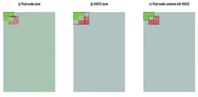
re-ecting biclusters. . . 17 2.5 Overlapped bicluster detection by the plaid
mod-el and HSSVD. In panmod-el (a), we draw the orig-inal data and the plaid model detection result is highlighted with a black frame. In panel (b), the HSSVD detection result is highlighted with a black frame. In panel (c), we obtain the mean approximation by HSSVD rst and then apply the plaid model detection result onto the mean
2.6 The image of raw data for Example 1. There are ve biclusters. Red is for positive values and
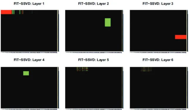
green is for negative values. . . 21 2.7 FIT-SSVD for Example1. Each layer represents
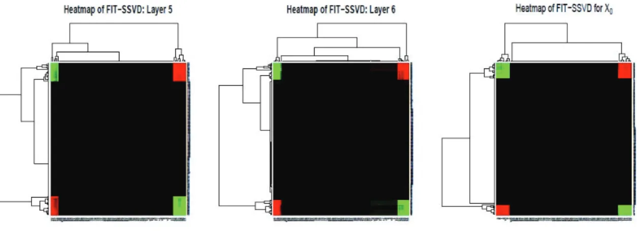
one bicluster. Layer 5 and 6 are pseudo mean biclusters. . . 22 2.8 Heatmaps of two pseudo mean biclusters and a
true mean bicluster. The rows and columns are reorders by hieratical clustering. Only the rst 200 rows (original order) are shown for better
display (the remaining rows are all 0). . . 23 2.9 HSSVD results for Example 1. Each layer
rep-resents one bicluster. There are four mean
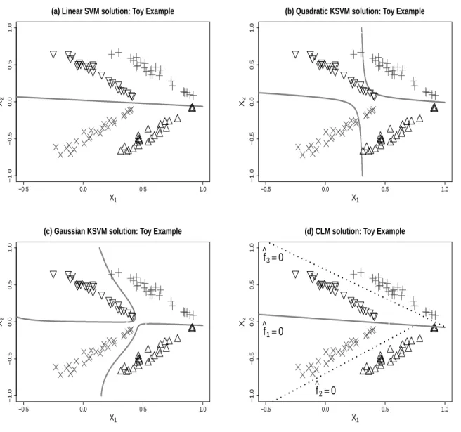
bi-clusters and two variance bibi-clusters. . . 24 3.1 Illustration of a two dimensional toy example. Grey
(+and×) represents the positive class and black (∇
and △) represents the negative class. In panels (a), (b) and (c), the decision boundaries are drawn with wide grey lines. In panel (d) for the CLM method, the wide grey line splits the data into two parts and in each part the dashed line is the separating
hyper-plane for the corresponding classier.. . . 30 3.2 Plots for CLM methods in twisted and
paral-lel cases. Black color (+ and ×) represents the positive class and grey color (∇ and △ repre-sents the negative class. Dierent symbols in the same class indicates the latent subclasses. In both panels (a) and (b), the boundary of fˆ1 is shown as a solid line and the boundaries of
ˆ
f2 and fˆ3 are given as dashed lines. In panels
(c) and (d), we show projections onto the space spanned by the rst 2principle components for the twisted and parallel cases. We apply PCA on the data which contains the informative vari-ables X1 and X2 as well as an additional 998
noise variables. The four-clusters structure in the original space (as observed in panels (a) and
3.3 Visualization of latent subclasses in the ovari-an covari-ancer dataset. The x-axis is the fˆ1 value, the y-axis displays the fˆ
2 value of the points
for which fˆ
1 is less than 0, otherwise it displays
the fˆ3 value. The plot indicates that there ex-ist subclasses within both the proliferative and
immunoreactive types of ovarian cancer. . . 51 3.4 Heatmap of ovarian cancer data using 153
ac-tive genes selected by sparse CLM with LUM loss. Samples are displayed in columns by sub-types. Genes are ordered by hierarchical cluster-ing. Nearly all samples on the left of the red line have average f1 greater than 0, and the
remain-ing samples have average f1 less than 0. We can
see a clear distinction between Imm(A) and Im-m(B), and a mild dierence between Pro(A) and Pro(B), which suggests that subclasses exist in
CHAPTER1: INTRODUCTION
With the revolutions in technology and science, we are now entering the era of Big Data. The enrichment of data promises achievement of many biological, medical, and public health goals. However, reaching these goals is challenging due to the increasing magnitude and complexity of the data. An important aspect of the complexity is data heterogeneity. Ignoring data heterogeneity can cause bias in making decisions. This is a common problem in modern biological and biomedical research, e.g. the one-size-t-all treatment strategy can fail due to heterogeneous response to drugs among patients. To deal with data heterogeneity, I have developed statistical learning and data mining methods under various heterogeneity settings. These methods are applicable for a wide range of problemspotentially high dimensionalwith direct interest to clinicians and biomedical investigators.
rule using training data where patients are potentially treated with sub-optimal doses. Information such as patient characteristics and outcome after receiving the dose are used as tailoring variables. This kind of problem can be viewed as a semi-supervised learning problem. Unlike the traditional semi-supervised learning problem where some observations have accurate labels and others have no labels, all observations are pro-vided with the label information (observed dose). However, such label information is not precise since the observed dose is generally suboptimal. Our proposed approach at-tempts to directly identify the dose rule which takes patient heterogeneity of response to treatment into account (see Chapter 4). All of our methods connect to existing statistical learning methods (Hastie et al. 2009) and are problem oriented.
CHAPTER2: BICLUSTERING WITH HETEROGENEOUS VARIANCE
In cancer research, as in all of medicine, it is important to classify patients into etiologically and therapeutically relevant subtypes to improve diagnosis and treatment. One way to do this is to use clustering methods to nd subgroups of homogeneous individuals based on genetic proles together with heuristic clinical analysis. A notable drawback of existing clustering methods is that they ignore the possibility that the vari-ance of gene expression prole measurements can be heterogeneous across subgroups, and methods that do not consider heterogeneity of variance can lead to inaccurate sub-group prediction. Research has shown that hypervariability is a common feature among cancer subtypes. In this chapter, we present a statistical approach that can capture both mean and variance structure in genetic data. We demonstrate the strength of our method in both synthetic data and in two cancer data sets. In particular, our method conrms the hypervariability of methylation level in cancer patients, and it detects clearer subgroup patterns in lung cancer data (see Chen et al. (2013)).
2.1 Introduction
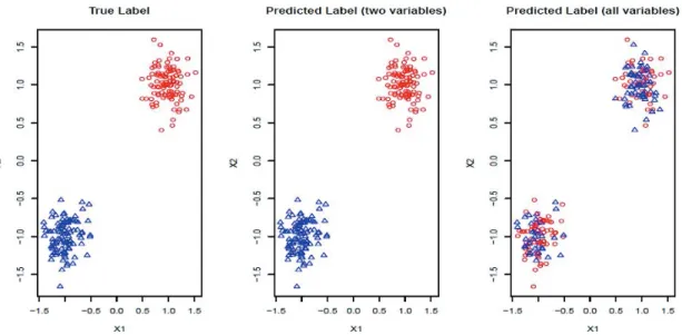
homogeneous groups by minimizing the summation of within clusters sum of squares (the Euclidean distances) of their gene expression proles. Unfortunately, this strategy is ineective when only a subset of features are informative. This phenomenon can be demonstrated by K-means clustering (Hastie et al. 2009) results for a toy example using only the variables which determine the underlying true cluster compared to using all variables (which includes many uninformative variables). As can be seen in Figure 2.1, clustering performance is poor when all variables are used in the clustering algorithm (Witten and Tibshirani 2010).
Figure 2.1: The data set contains two clusters determined by two variables X1 and
X2 such that points around (1,1)and (−1,−1)naturally form clusters. There are 200
observations (100 for each cluster) and 1002 variables (X1, X2 and 1000 random noise
variables). We plot the data in the 2D space of X1 and X2. The graphs with true
cluster labels and predicted cluster labels obtained by clustering using onlyX1 and X2
and clustering by using all variables are laid from left to right. The predicted labels are the same as the true labels only whenX1 and X2 are used for clustering; however,
the performance is much worse when all variables are used.
Huang 2008, Zou et al. 2006) and Sparse K-means (Witten and Tibshirani 2010), among others (Kriegel et al. 2009). However, sparse clustering still fails if the true sparsity is a local rather than a global phenomenon (Kriegel et al. 2009). More specically, dierent subsets of features can be informative for some samples but not all samples, or, in other words, sparsity exists in both features and samples jointly. Biclustering methods are a potential solution to this problem, and further generalize the sparsity principle by considering samples and features as exchangeable concepts to handle local sparsity (Cheng and Church 2000, Kriegel et al. 2009). For example, gene expression data can be represented as a matrix with genes as columns, and subjects as rows (with various and possibly unknown diseases or tissue types). Traditional methods will either cluster the rowsas done, for example, in microarray research, where researchers want to nd subpopulation structure among subjects to identify possible common disease statusor cluster the columns, as done, for example, in gene clustering research, where genes are of interest and the goal is to predict the biological function of novel genes from the function of other well studied genes within the same clusters. In contrast, biclustering involves clustering rows and columns simultaneously in order to account for the interaction of row and column sparsity. This local sparsity perspective provides an intuition for using sparse singular value decomposition algorithms (SSVD) for bi-clustering Busygin et al. (2002), Lee et al. (2010), Yang et al. (2014), Witten et al. (2009). SSVD assumes that the signal in the data matrix can be represented by a low rank matrix X≈ UDVT =∑r
i=1diuivTi with X ∈ ℜn×p. U= [u1,u2, . . . ,ur] ∈ ℜn×r
and V = [v1, v2, . . . ,vr] ∈ ℜr×p contain left and right sparse singular vectors and
are orthonormal with only a few non-zero elements (corresponding to local sparsity). D∈ ℜr×r is diagonal (with diagonal elements d
1, d2, . . . , dr) with r << rank(X). The
outer product of each pair of sparse singular vectors (uivTi ,i= 1,2, . . . , r) will designate
A common assumption of existing SSVD biclustering methods is that the observed data can be decomposed into a signal matrix plus a fully exchangeable random noise matrix:
X=Ξ+Φ, (2.1)
whereX is the observed data,Ξ= (ξij)is ann×pmatrix representing the signal, and Φ= (ϕij)is ann×prandom noise/residual matrix with i.i.d. entries (Yang et al. 2014,
Ho 2010, Johnstone and Lu 2009). A method based on model (2.1) is proposed in Lee et al. (2010) which minimizes the sum of the Frobenius norm of X−Ξˆ and a penalty function with variable selection, such as the ℓ1−norm (Tibshirani 1994) or SCAD
(Fan and Li 2001). A similar Loss plus Penalty minimization approach can be seen in Witten et al. (2009). A dierent method for SSVD employs iterative thresholding QR decomposition to estimate Ξˆ in Yang et al. (2014). We refer to Lee et al. (2010) as LSHM and Yang et al. (2014) as FIT-SSVD, and compare these approaches to our method. An alternative approach, which is more direct, is based on a mixture model (Lazzeroni and Owen 2002, Shabalin et al. 2009). For example, Shabalin et al. (2009) denes the bicluster as a submatrix with a large positive or negative mean. Although these approaches have proven successful in some settings, they are limited by their focus on only the mean signal approximation. In addition, the explicit homogeneous residual variance assumption is too restrictive in many applications.
given above (Allen et al. 2014). Drawbacks of the generalized PCA method, however, are that it remains focused on mean signal approximation and the structure of R−1 and Q−1 must be explicitly known in advance.
In this chapter, we present a new biclustering framework based on sparse sin-gular value decomposition called heterogeneous sparse sinsin-gular value decomposition (HSSVD). This method can detect both mean biclusters and variance biclusters in the presence of unknown heterogeneous residual variance. To our knowledge, both the heterogeneous residual variance and variance only bicluster detection aspects are com-pletely novel. We also apply our method, as well as competing approaches, to two cancer data sets, one with methylation data and the other with gene expression data. Our method delivers better pattern detection and is able to conrm the biological nd-ings originally made for each of the data sets. We also apply our method to synthetic data to demonstrate its superior performance over competing approaches quantitative-ly. We demonstrate that our proposed method is robust, location and scale invariant, and computationally feasible.
2.2 Model Assumptions for HSSVD
We dene biclusters as subsets of the data matrix which have the same mean and variance. We assume that there exists a dominate null cluster in which all elements have a common mean and variance and that all other biclusters are restricted to rectangular structures which have either a distinct mean or variance compared to the null cluster. We can also express our model in the framework of a random eect model wherein
whereXand Ξare the same structures given in the traditional model (2.1), and where we require Φ, an n×p matrix, to have i.i.d. random components with mean 0 and variance 1. Moreover, the× in (2.2) is dened element wisely: see the next section for details. New components in the model includeΣ= (σij), ann×pmatrix representing
the heterogeneous variance signal;Jn×p, ann×pmatrix with all values equal to 1;ρ, a
nite positive number serving as a common scale factor; andb, a nite number serving as a common location factor. We also make the sparsity assumption that the majority of(ξij)values are 0and the majority of(σij)values are 1. Further, just as we assumed
for the mean structure Ξ, we also assume that the variance structure Φis low rank. From the denitions, the traditional model (2.1) is a special case of our model (2.2), with b = 0, Σ = J, and ρ = 1. The presence of b and ρ in the model allows the new method to be scale invariant, while the presence of Σ enables the new method to incorporate heterogeneous variance signals.
2.3 HSSVD method
We propose HSSVD based on the model (2.2) with a hierarchical structure for signal recovery. First, we properly scale the matrix elements to minimize false detection of pseudo mean biclusters which can arise as artifacts of high-variance clusters. This motivates us to add the quadratic rescaling step in the procedure. Then we can detect mean biclusters based on the scaled data and later detect variance biclusters based on the logarithm of the squared residual data after subtracting out the mean biclusters. The quadratic rescaling step works well in practice, as shown in the simulation studies and data analysis. The pseudo code for the algorithm is provided as follows:
1. Input Step: Input the raw data matrix Xorigin. Standardize Xorigin (treat each
cell as i.i.d.) to have mean 0and variance 1. Denote the overall mean ofXorigin
dened as X= (Xorigin−µˆJ)/ˆσ.
2. Quadratic Rescaling: Apply SSVD onX2−J to obtain the approximation matrix U.
3. Mean Search: Let Y = X/√U+J−cJ, where c is a small nonpositive con-stant to ensure that √U+J−cJ exists. Then apply SSVD on Y to obtain the approximation matrix Y˜.
4. Variance Search: Let Zorigin = log(X−Y˜ ×
√
U+J−cJ)2, centerZorigin to have
mean0, and denote the centered version asZ. Perform SSVD onZ to obtain the approximation matrix Z˜.
5. Background Estimation: Let P={pij} denote the n×p matrix of indicators of
whether the corresponding cells belong to the background cluster, with pij = 1
if both Y˜
ij = 0 and Z˜ij = 0, and pij = 0 otherwise. Based on the assumption
that most elements in the matrix should be in the null cluster, we can estimate ˆb with 1′(Xorigin×P)1
1′P 1 and ρˆwith
1′(Xorigin×P−ˆbP)21
1′P 1−1 , where 1 is a vector with all
elements equal to one.
6. Scale Back: Dene P1 = {pij}, with pij = 1 if Y˜ij = 0, pij = 0 otherwise.
Similarly, deneP2 ={pij}, withpij = 1 if Z˜ij = 0,pij = 0 otherwise. The mean
(Ξ+bJ) approximation is computed withσ( ˜ˆ Y×√U+J−cJ) + ˆµ(J−P1) +ˆbP1,
and the variance (ρ2Φ) approximation is computed with [ ˆρ2P
2+ˆσ2(J−P2)]×
exp( ˜Z).
The operators ×,/, exp(),log(), exp(), min() and √() used above are dened element wisely when they are applied to the matrix, e.g. Un×p×Vn×p =
(uijvij). In all steps involving sparse singular value decomposition, we implement the
and has similar or superior performance compared to other competing methods under the homogeneous variance assumption Yang et al. (2014). The matrix √U+J−cJ provides a working variance level estimate of the data and makes our method more robust. Note that the reason for working on the log scale for the variance detection is two fold. First, working on the log scale makes the detection of the deated variance (less than 1) bicluster possible. Intuitively, as variance measures deviance from the mean, we can work on the squared residuals to nd the variance structure. For the deated variance bicluster setting, if the mean structure is estimated correctly, the residuals within the bicluster are close to zero. The SSVD based methods shrink the small non-zero elements to zero to achieve sparsity. As a result, if we work on the squared residuals directly, the SSVD based methods will fail to detect the low variance structure. Second, to use the well-established SSVD method in the variance detection steps we need to work on the log scale. To see this, we can rewrite the equation in (2.2) as log(X−Ξ −bJ)2 = log(Σ2) + log(ρ2Φ2), which is similar to the model in
The FIT-SSVD method, as well as any other SVD based method, requires an ap-proximation of the rank of the matrix (which is essentially the number of true biclus-ters) as input. We adapt the bi-cross validation method (BCV) by Owen and Perry (2009) for rank estimation, and we notice that in some cases the rank is underestimat-ed. For this reason, we introduce additional steps following a BCV rank estimation of rank k: First, we approximate the data with a sparse matrix Xˆk+1 (rank =k+ 1),
where Xˆ
k+1 = ∑k+1
j=1dˆjuˆjvˆTj. Dene the proportion of variance explained by the top
i rank sparse matrix as Ri =
∑i j=1dˆ
2
j/
∑k+1
j=1dˆ 2
j (Allen and Maletic-Savatic 2011). Ri
is between 0 and 1 and is increasing with i, and we believe that the redundant com-ponents of the sparse matrix should not contribute much to the total variance. The nal rank estimation for HSSVD is the smallest integerrwhich satisesRr >0.95, and
1≤r ≤k+ 1. Note that FIT-SSVD (Yang et al. 2014) used the modied BCV method for rank estimation, however, the authors require that most rows (the whole row) and most columns (the whole column) are sparse, which appears to be too restrictive. In practice, this assumption is violated if the data is block diagonal or has certain other commonly assumed data structures. For this reason, we use the original BCV method as our starting point.
2.4 Application to cancer data
2.4.1 Hypervariability of methylation in cancer
lung, thyroid and Wilms' tumor cancers) and matched normal samples. Each sample had 384 methylation probes which covered 151 cDMRs. The authors of the primary report concluded that cancer samples had hypervariability in these cDMRs across all cancer types (Hansen et al. 2011).
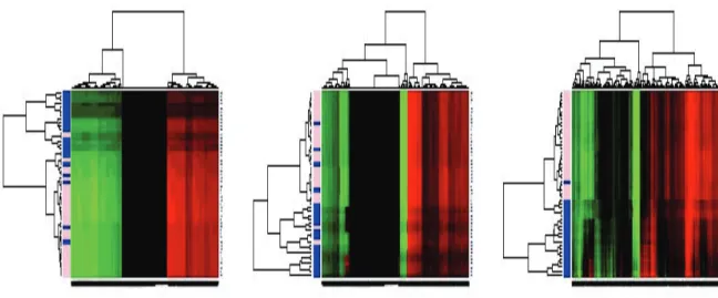
First, we wish to verify that HSSVD can provide a good mean signal approximation of methylation. In this data set, all the probes measuring the methylation are placed in the cDMRs identied in colon cancer patients. As a result, we would expect that mean methylation levels dier between colon cancer samples and the matched normal sam-ples. Under this assumption, we require the biclustering methods to capture this mean structure before investigating the information gained from variance structure estima-tion. Note that the numerical range of methylation level is between0and 1. Hence we applied the logit transformation on the original data for further biclustering analysis. We compare three methods, HSSVD, FIT-SSVD and LSHM; all based on SVD. Only colon cancer samples and their matched normal samples are used for this particular analysis. In Figure 2.2, we can see from the hierarchical clustering analysis that the majority of colon cancer samples (labeled blue in the side bar) are grouped together and most of the cDMRs are dierentially expressed in colon tumor samples compared to normal samples. The conclusion is the same for all three methods compared, including our proposed HSSVD method.
Figure 2.2: Mean Approximation of colon cancer and the normal matched samples. From left to right the methods are HSSVD, FIT-SSVD and LSHM. The colon cancer samples are labeled in blue, and the normal matched samples are labeled in pink in the sidebar. The genes and samples are ordered by hierarchical clustering. The colon cancer patients are clustered together which indicates the mean approximations for these three methods achieves the expected signal structure.
their mean level methylation varies from sample to sample. Hence, identifying variance biclusters can provide potential new insight for cancer epigenesis.
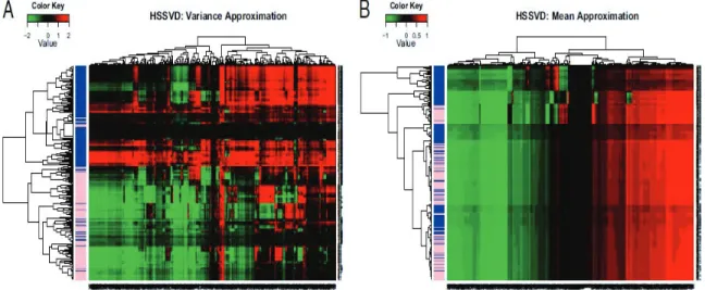
Figure 2.3: HSSVD approximation result for all samples. The variance approximation is in panel (a) and the mean approximation is in panel (b). Blue represents cancer samples, and pink represents normal samples in the sidebar. The genes and samples are ordered by hierarchical clustering. Red color represents large values, and green color represents small values. Only the variance approximation can discriminate between cancer and normal samples. More importantly, within the same gene, the heatmap for the variance approximation indicates that cancer patients have larger variance than normal individuals. This result matches the conclusion in Hansen et al. (2011). In addition, the cDMRs with the greatest contrast variance across cancer and normal samples are highlighted by the variance approximation, while the original paper does not provide such information.
2.4.2 Gene expression in lung cancer
studied in the statistics literature (Lee et al. 2010, Shabalin et al. 2009, Yang et al. 2014). The samples are a subset of patients (Liu et al. 2008) having lung cancer with gene expression measured by the Aymetrix 95av2 GeneChip (Bhattacharjee et al. 2001). The data set contains the expression levels of12,625genes for 56patients, each having one of four disease subtypes: normal lung (20 samples), pulmonary carcinoid tumors (13samples), colon metastases (17samples), and small cell carcinoma (6samples).
The performance of dierent methods is evaluated based on the pattern dierence of subtypes based on the mean approximations. For all methods, we set the rank of the mean signal matrix equal to 3 to maintain consistency with the ranks used in FIT-SSVD (Yang et al. 2014) and LSHM (Lee et al. 2010). Further, we use the measurement support to evaluate the sparsity of the estimated gene signal (Yang et al. 2014). Support is the cardinality of the non-zero elements in the right and left singular vectors across the three layers (i.e., support is an integer that cannot exceed the data dimension). Smaller support values suggest a sparser model. Table 2.1 shows that HSSVD, FIT-SSVD and LSHM yield similar levels of sparsity in the gene signal, while SVD is not sparse, as expected. Figure 2.4 shows checkerboard plots of rank-three approximations by the four methods. Patients are placed on the vertical axis, and the patient order is the same for all images. Patients within the same subtype are stacked together and dierent subtypes are separated by white lines. Within each image, genes are laid on the horizontal axis and are ordered by the value ofvˆ2 (Yang et al. 2014). We
Table 2.1: Lung cancer: summary of cardinality of union support of the rst three singular vectors for dierent methods
HSSVD FIT-SSVD LSHM SVD ∪3
i=1∥ui∥0 4689 4686 4655 12625
∪3
i=1∥vi∥0 56 56 56 56
2.5 Simulation study
To evaluate the performance of HSSVD quantitatively, we conducted a simulation study. We compared HSSVD with the most relevant existing biclustering methods, FIT-SSVD and LSHM Yang et al. (2014), Lee et al. (2010). HSSVD includes a rank estimation component, while the other methods do not automatically include this. For this reason, we will use a xed oracle rank (at the true value) for the non-HSSVD methods. For comparison, we also evaluate HSSVD with xed oracle rank (HSSVD-O). The performance of these methods on simulated data was evaluated on four criteria. The rst criterion is sparsity of estimation, dened as the ratio between the size of the correctly identied background cluster and the size of the true background cluster. The second criterion is biclustering detection rate, dened as the ratio of the intersection of the estimated bicluster and the true bicluster over their union (also known as the Jaccard index). For the rst two criteria, larger values indicate better performance. The third and fourth criteria are overall matrix approximation errors for mean and variance biclusters, consisting of the scaled recovery error for the low-rank mean signal matrix Ξ˜ =Ξ+bJ, computed via
Lmean( ˜Ξ,Ξˆ) =∥Ξˆ −Ξ˜∥2F/∥Ξ∥
2
F;
Figure 2.4: Checkerboard plots for four methods. We plot the rank-three approximation for each method. Within each image, samples are laid in rows, and genes are in columns. We order the samples by subtype for all images (top to bottom: Carcinoid, Colon, Normal, and Smallcell), and dierent subtypes are separated by white lines. Genes are sorted by the estimated second right singular vector (uˆ2), and we only included genes
that are in the support (dened in Table 2.1). Across all methods, the HSSVD and FIT-SSVD methods provide the clearest block structure reecting biclusters.
log(ρ2J), computed via
Lvar(log( ˜Σ),log( ˆΣ)) = ∥log( ˆΣ
1/2
)−log( ˜Σ1/2)∥2F/∥log(Σ1/2)∥2F,
with ∥.∥F being the Frobenius norm.
The simulated data comprise a 1000×100 matrix with independent entries. The background entries follow a normal distribution with mean 1 and standard deviation 2. We denote the distribution asN(1,22), whereN(a, b2) represents a normal random
bicluster 3 is a mean and small variance cluster, and bicluster 4 is a large variance cluster. More precisely, bicluster1(size 100×20) is generated fromN(7,22), bicluster 2 (size 100×10) is generated from N(−5,22), bicluster 3 (size 100×10) is generated
from N(7,0.42), bicluster 4 (size 100×20) is generated from N(1,82), and bicluster
5 (size 100×20) is generated from N(6.8,22). The biclustering results are shown in
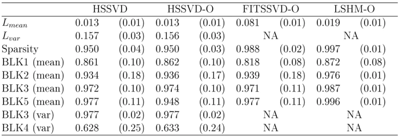
Table 2.2: HSSVD and HSSVD-O can detect both mean and variance biclusters, while FIT-SSVD-O and LSHM-O can only detect mean biclusters. For mean bicluster detec-tion, all methods performed well since the biclustering detection rates are all greater than 0.7. For variance bicluster detection, HSSVD and HSSVD-O deliver a similar biclustering detection rate. On average, the computation time of LSHM-O is about 30times that of HSSVD and 60 times that of FIT-SSVD-O.
Table 2.2: Comparison of four methods in the simulation study. TheLmeanand Lvar is
measuring the dierence between the approximated signal and the true signal, and so smaller is better. For the other measures of accuracy of bicluster detection, the larger the better. The rows BLK1 to BLK5 represent the biclustering detection rate for each bicluster.-O indicates that the oracle rank is provided.
HSSVD HSSVD-O FITSSVD-O LSHM-O
Lmean 0.013 (0.01) 0.013 (0.01) 0.081 (0.01) 0.019 (0.01)
Lvar 0.157 (0.03) 0.156 (0.03) NA NA
Sparsity 0.950 (0.04) 0.950 (0.03) 0.988 (0.02) 0.997 (0.01) BLK1 (mean) 0.861 (0.10) 0.862 (0.10) 0.818 (0.08) 0.872 (0.08) BLK2 (mean) 0.934 (0.18) 0.936 (0.17) 0.939 (0.18) 0.976 (0.01) BLK3 (mean) 0.972 (0.10) 0.974 (0.10) 0.971 (0.11) 0.987 (0.01) BLK5 (mean) 0.977 (0.11) 0.948 (0.11) 0.977 (0.11) 0.996 (0.01)
BLK3 (var) 0.977 (0.02) 0.977 (0.02) NA NA
BLK4 (var) 0.628 (0.25) 0.633 (0.24) NA NA
2.6 Properties of HSSVD
2.6.1 HSSVD as a denoising procedure
We study overlapped mean bicluster detection through a simulated example. The plaid model is usually preferred to SVD based methods for overlapped mean bicluster detection, although the plaid model (Lazzeroni and Owen 2002, Turner et al. 2005) can be sensitive to variance heterogeneity. We want to show that our method as an SVD based method is still useful for overlapped mean bicluster detection as a denois-ing step. First, we represent the data in a 200×100 matrix. The elements in the null cluster followN(0,12). At the same time, we have two overlapping biclusters with
their sizes both equal to 20×20. The elements in the two biclusters follow N(7,22)
andN(−5,32), respectively, and the overlapped block size is10×10. Hence, under the
rst apply HSSVD to obtain a mean approximation of the raw data and then apply the plaid model to the mean approximation to detect biclusters. We utilize the BCPlaid function in the R package biclust (http://CRAN.R-project.org/package=biclust) as the implementation of the plaid model (Lazzeroni and Owen 2002, Turner et al. 2005). The graphical results are presented in Figure 2.5. The detected biclusters are highlight-ed by a black frame. From Figure 2.5 (b), we see that although sparse singular value decomposition is good at mean signal approximation for non-overlapping bi-clusters, it cannot recover the true overlapped bicluster structure. Meanwhile, we can see that after applying HSSVD, the plaid model (Figure 2.5 (c)) successfully picks out the un-derlying true structure, while applying the plaid model alone (Figure 2.5 (a)) was not successful. This result implies that for overlapped mean bicluster detection, the plaid model is generally better, but when there is variance heterogeneity present, the HSSVD can be quite helpful as a denoising process.
2.6.2 The necessity of the variance detection step in HSSVD
As we assume a low rank structure in both mean signal and variance signal, a natural question to ask is whether such a structure can be approximated well by a higher-rank matrix for the mean structure only. In other words, can we represent the variance biclusters by using pseudo-mean biclusters. Our conclusion is that it is improper to use mean biclusters for variance bicluster detection. Pseudo-mean biclusters cannot recover the small variance biclusters at all, due to the natural shrinkage inherent in sparse singular value decomposition methods. Further, we will show that pseudo-mean biclusters can reveal some structure for the large variance biclusters, however the approximation is rough. Consider the simulation data in Example1(see Figure 2.6 for graphical display).
Figure 2.5: Overlapped bicluster detection by the plaid model and HSSVD. In panel (a), we draw the original data and the plaid model detection result is highlighted with a black frame. In panel (b), the HSSVD detection result is highlighted with a black frame. In panel (c), we obtain the mean approximation by HSSVD rst and then apply the plaid model detection result onto the mean approximation data.
with input rank equal to 6 versus HSSVD with an estimated rank (in Figure 2.9). We can see that there are four mean biclusters from Figure 2.6. As the input rank is greater than the mean bicluster number, there will be several pseudo-mean biclusters (layer 5 and layer 6) in the FIT-SSVD result. For HSSVD, there will be both mean biclusters and variance biclusters. In Figure 2.7, it appears that the pseudo mean biclusters can detect part of the variance biclusters, however, this is because we know the correct order to display the graph. However, in practice, we would not know this order. Moreover, we can see that the pseudo-mean structure can be confounded with a type of true bicluster.
Figure 2.7: FIT-SSVD for Example1. Each layer represents one bicluster. Layer5and 6are pseudo mean biclusters.
For example, let X0 = uvT + Φ ,u = (rep(1,50),rep(1,50),rep(0,900)), v =
(rep(1,5),rep(−1,5),rep(0,90)), where rep(1,5) = (1,1,1,1,1) and Φ is a 1000 ma-trix with entries follow i.i.d N(0,1). There is only a mean bicluster for X0, and we can
for X0 and the pseudo-mean biclusters, layer 5 or layer 6 for Example 1, graphically,
the resulting heatmaps, given in Figure 2.8 (rows and columns are reordered by hier-archical clustering), are very similar. This indicates that pseudo-mean biclusters can be confounded with certain true mean biclusters. This issue is probably even more complicated for real data settings.
Figure 2.8: Heatmaps of two pseudo mean biclusters and a true mean bicluster. The rows and columns are reorders by hieratical clustering. Only the rst200rows (original order) are shown for better display (the remaining rows are all 0).
In contrast, HSSVD can provide more accurate large variance bicluster detection (layer 1 for variance) and small variance bicluster detection (layer 2 for variance), as shown in Figure 2.9. Lastly, we want to emphasize that the BCV method (Owen and Perry 2009) can be quite helpful for preventing the type of pseudo-mean detection which can weaken variance detection in the latter steps.
2.7 Conclusion and Discussion
Figure 2.9: HSSVD results for Example 1. Each layer represents one bicluster. There are four mean biclusters and two variance biclusters.
has the advantage of working on the log scale in estimating the variance components: the log scale makes detection of low variance (less than 1) biclusters possible, and any traditional sparse singular value decomposition method can be naturally utilized in our variance detection steps. The new method conrms the existence of methylation hy-pervariability in the methylation data example, something which cannot be done with other existing biclustering methods. Although we use the FIT-SSVD method in our im-plementation, other low rank matrix approximation methods are applicable. Moreover, the software implementing our proposed approach was computationally comparable to the other approaches we evaluated.
on the raw data to obtain the mean approximation. Then we can apply a suitable ap-proach, such as the widely used plaid model (Lazzeroni and Owen 2002, Turner et al. 2005), on the mean approximation to detect overlapping biclusters. This combined procedure improves on the performance of the plaid model when the overlapping bi-clusters have heterogeneous variance. Hence our method remains useful in the present of overlapping biclusters.
Another potential issue for HSSVD is the question of whether a low rank mean ap-proximation plus a low rank variance apap-proximation could be alternatively represented by a higher rank mean approximation. In another words, is it possible to detect variance biclusters through mean biclusters only, even though the mean clusters which form the variance clusters would be pseudo-mean clusters. Our conclusion is that the variance detection step in HSSVD is necessary for the following two reasons: First, pseudo-mean biclusters are completely unable to capture small variance biclusters. Second, although pseudo-mean biclusters are able to capture some structure from large variance biclus-ters, such structure is much less accurate than that provided by HSSVD, and can be confounded with one or more true mean biclusters.
CHAPTER3: COMPOSITE LARGE MARGIN CLASSIFIERS WITH LATENT SUBCLASSES
3.1 Introduction
since dierent cancer subtypes can have heterogenous response to treatment (Liu et al. 2010, Lehmann et al. 2011). In general, complex examples with data heterogeneity such as AD and cancer subtype classication can pose challenges for linear classiers because of their insucient exibility for capturing potential data heterogeneity.
To further illustrate the problem of interest, we show a simple two dimensional toy example in Figure 3.1. This is a binary classication problem with X1 and X2 as
pre-dictors, and two classes are labeled in grey plus and black cross signs. As we can see from the plots, each class has two latent subclasses. A linear SVM model is tted to the data and its decision boundary is shown in the solid line in Figure 3.1(a). Note that although linear methods for classication are not able to eectively capture the dierence between classes in this example, the classication task becomes much easier if we divide the data by the lineX2 = 0. In practice, when in-class heterogeneity is
ig-nored, traditional procedure may have poor classication performance. This motivates us to introduce the idea of a splitting function to divide the data into two parts so that we can handle the classication task with two separate linear classiers.
SVMs work reasonably well. However, their decision boundaries are quite complicat-ed. Moreover, we will show in Section 3.4 that the performance of kernel SVMs can deteriorate rapidly when the dimension of covariates increases.
To solve the classication problem for complex structures, we propose a new group of methods, namely the Composite Large Margin Classier (CLM). The CLM aims to nd three linear functions simultaneously: one linear function to split the data into two parts, with each part being classied by a dierent linear classier. We denote these three linear functions as f1(x), f2(x), f3(x), respectively. Because of the split
function, the CLM method provides a natural solution to the classication problem with latent subgroups. In Figure 3.1(d), we plot the decision boundary of the CLM withfˆ1(x) = 0 using a solid line, and bothfˆ2(x) = 0and fˆ3(x) = 0 using dashed lines. The function fˆ
1(x) helps capture the hidden structure and divide the data into two
parts, one part with fˆ
1(x) >0 and the other part with fˆ1(x) <0. With this division,
we can use two separate linear classiers on each part. In particular, we predict the label yˆ=sign( ˆf2(x)) for the part on the top, and yˆ=sign( ˆf3(x)) for the part on the
bottom. Thus, our CLM method makes use of three linear functions simultaneously to classify the data and capture the latent subclasses.
−0.5 0.0 0.5 1.0 −1.0 −0.5 0.0 0.5 1.0
(a) Linear SVM solution: Toy Example
X1
X2
−0.5 0.0 0.5 1.0
−1.0
−0.5
0.0
0.5
1.0
(b) Quadratic KSVM solution: Toy Example
X1
X2
0
0
−0.5 0.0 0.5 1.0
−1.0
−0.5
0.0
0.5
1.0
(c) Gaussian KSVM solution: Toy Example
X1
X
2
0 0
−0.5 0.0 0.5 1.0
−1.0
−0.5
0.0
0.5
1.0
(d) CLM solution: Toy Example
X1 X 2 0 f ^
1=0
f ^
2=0
f ^
3=0
Figure 3.1: Illustration of a two dimensional toy example. Grey (+ and ×) represents the
positive class and black (∇ and △) represents the negative class. In panels (a), (b) and (c), the decision boundaries are drawn with wide grey lines. In panel (d) for the CLM method, the wide grey line splits the data into two parts and in each part the dashed line is the separating hyperplane for the corresponding classier.
Although our CLM method is motivated by large margin classiers, the funda-mental concept is more general and can be applied to many other linear classiers as well. Furthermore, besides classication, we can also generalize the CLM method to regression. In this article, we only focus on the implementation of the LUM loss and the logistic loss for classication and use them as examples to illustrate how the CLM method works.
The rest of chapter is organized as follows. In Section 3.2.1, we briey review binary classication methods. The CLM framework is introduced in Section 3.2.2 and the properties of the CLM and its connection to existing methods are discussed in Section 3.2.3. In Section 3.3, we present a principal component analysis (PCA) based computational strategy for non-sparse solutions and a retting procedure for sparse solutions. We demonstrate the eectiveness of our method with simulated data and the apply the method to the analysis of Alzheimer's disease and cancer data in Sections 3.4 and 3.6, respectively. Concluding comments are given in Section 3.7.
3.2 Methodology
We rst review binary classication and large margin classiers in Section 3.2.1. Due to the limitation of existing large margin classiers for classication with latent subclasses, we propose the Composite Large Margin (CLM) classier in Section 3.2.2. Furthermore, we discuss the properties of the CLM with two particular loss functions, the LUM and logistic losses, in Section 3.2.3.
3.2.1 Review of Binary Classication
Suppose we have a training data set {(xi, yi);i = 1,2, . . . n} available. The class
given binary classication problem, there are many techniques available in the literature and our focus in this chapter is on large margin classiers (Hastie et al. 2009). Given the training data set, a large margin classier is trained to obtain f(x) : ℜk → ℜ,
such that the predicted class label is assigned using the sign of f(x). Note that we correctly predict the class label ofxwhen yf(x) is positive. The term yf(x) is known as the functional margin. In general, the objective function of a large margin classier can be written in the regularization framework of a loss plus a penalty. The loss is a measure of the goodness of t between the model and data, and the penalty controls the complexity of the model to avoid overtting. Specically, the optimization problem of a large margin classier can be expressed as follows:
min
f∈FJ(f) +λ n
∑
i=1
L(yif(xi)),
where F is the function class that all candidate solution functions belong to, J(f) is a regularization term penalizing the complexity of f, L(·) is the loss function, and λ is a tuning parameter balancing the two terms. When the function f(x) is linear with the form wT x, a common choice of J(f) is the ℓ2 penalty, i.e. ∥w∥22. A natural loss
function is the so called 0−1 loss with value 1 if yf(x) ≤ 0, and 0 otherwise, i.e. L0−1(yf(x)) = I{yf(x) ≤ 0}. However, the 0−1 loss is dicult for optimization
due to its nonconvexity. Consequently, various convex surrogate loss functions have been proposed in the literature to alleviate the computational problem (Zhang 2004). For example, SVM uses hinge loss, penalized logistic regression uses logistic loss, and AdaBoost uses exponential loss (Friedman et al. 2000).
LUM loss function in detail. The LUM loss is indexed by two parameters aand cwith the following explicit form:
V(u) =
1−u if u≤ 1+cc,
1 1+c(
a
(1+c)u−c+a)
a if u > c
1+c.
(3.1)
The left piece of V(u) with u ≤ 1+cc is the same as the hinge loss used in the SVM. The right piece is a convex curve whose shape is controlled by c with rate of decay controlled by a. With a > 0 and c → ∞, LUM is equivalent to standard SVM. With a→ ∞ and xedc, LUM loss is a hybrid of SVM and AdaBoost.
The techniques discussed above work well in many traditional classication prob-lems. For large margin classiers, it is common to use linear learning. One advantage of linear learning is its simple interpretation. Once the functionf(x) =xT wis obtained,
one can examine the importance of each dimension inxthrough its corresponding coef-cientsw. When a linear function is insucient, one can map the original linear space to a higher dimensional nonlinear space using kernel methods (Hastie et al. 2009). De-spite its exibility, it is typically more dicult to interpret. Our goal is to propose a class of classiers which maintain sucient exibility to incorporate latent subclasses without losing the interpretability of linear classiers.
3.2.2 The Composite Large Margin (CLM) framework
In this section, we describe the CLM framework for binary classication with latent subclasses in detail. We assume there does not exist a global single linear classier that can well separate the positive and the negative classes due to the existence of heterogenous subclasses. However, the data can be divided by a simple function (e.g. a linear function) into two parts, and each part can be classied relatively easily.
generalized 0−1 latent classication loss as W0−1(y,x) = I(f1(x) ≤ 0)I(yf2(x) ≤
0) +I(f1(x) > 0)I(yf3(x) ≤ 0), where f1(x) is the splitting function, f2(x) is the
classier for data points withf1(x)≤0, andf3(x)is the classier for data points with
f1(x)>0.
The generalized0−1latent classication loss is the composition of two0−1standard binary classication loss functions with weightsI(f1(x)≤0)and I(f1(x)>0). Similar
to the standard 0−1 loss, it is hard to optimize the generalized 0− 1 loss due to its discontinuity. In practice, a surrogate loss function is often used instead. For illustration, we use logistic and LUM losses as surrogate loss functions for the indicators I(yf2(x)≤0) and I(yf3(x)≤0). For weight functionsI(f1(x)≤0) and I(f1(x)>0),
we use G(−f1(x)) and G(f1(x))as their corresponding smooth approximations, where
G(u) is dened as:
G(u) =
1 if u≥ϵ,
1−0.5(1−u/ϵ)2 0≤u≤ϵ
0.5(1 +u/ϵ)2 −ϵ≤u≤0
0 u≤ −ϵ.
(3.2)
ϵis tuning parameter, but we can set it to be small. Note thatG(u) +G(−u) = 1, also asϵ →0, G(u) converges to I(u >0)pointwisely. Note that this choice is not unique, and there are many other possible approximations such as sigmoid functions.
The loss functions Wlog and Wlum for the latent classication problem are dened
as follows:
Wlum(yi,xi) = αiV
(
yif2(xi)
)
+ (1−αi)V
(
yif3(xi)
)
, (3.3)
where αi = G(−f1(xi)). Note that the Wlog and Wlum losses are the compositions of
two logistic and LUM loss functions, respectively. The αi and 1−αi are the weights.
Furthermore, We assume thatf1,f2,f3 are all linear, i.e. fj(x) =x wTj +bj, j = 1,2,3,
to maintain the interpretability of linear classiers.
With the loss function L(y,x) dened, we can express the optimization problem for CLM as minw,bQ(w,b|Y,X) = 12
∑3
j=1||wj||22+λ ∑n
i=1L(yi,xi), where λ is the
tuning parameter, and (w,b) = (w1,w2,w3, b1, b2, b3). We will discuss the algorithm
for obtaining the CLM solution in Section 3.3. Next, we briey describe the properties of the CLM method.
3.2.3 Connections with existing literature
To handle the data heterogeneity and identify the potential subtypes, there are two main categories of methods in the literature. One is tree-based methods (Breiman et al. 1984), and the other is likelihood based mixture models (Fraley and Raftery 2002).
For tree-based methods, several techniques (Kim and Loh 2001, Loh 2010) were pro-posed to overcome the potential problems of splitting variables with only local eects. For example, GUIDE allows searching for linear splits using two variables at one time when the marginal eects of both covariates are weak, while the pairwise interaction eect is strong (Loh 2010). Both GUIDE and CLM can work well for certain problems as illustrated in Section 3.4, while traditional tree-based methods cannot. Unlike the tree-based GUIDE, CLM is a composite large margin classier motivated by latent variables. Furthermore, with the use of three linear functions, the interpretation of CLM is relatively simple. Lastly, our numerical examples indicate that CLM is more competitive for high dimensional data.
has a hierarchical structure. The hierarchical mixture of experts (HME) introduced by Jordan and Jacobs (1994) is one such example described as follows. Assume that there are two layers and four components. Then, the parametric likelihood ofY given X can be written as:
P(Y|X, θ) =
2 ∑
i=1
g(i)
2 ∑
j=1
g(j|i)µIij(y=1)(1−µij)I(y=−1),
whereg(i) = exp(qi(x, θ))/(exp(q1(x, θ)) + exp(q2(x, θ))),
g(j|i) = exp(qj|i(x))/(exp(q1|i(x, θ)) + exp(q2|i(x, θ))), µij =E(I(Y = 1)|i, j, X, θ).
The g(i) and g(j|i)are the proportions for the four components, and µij is the model
for a given component. The task is to calculate the MLE for θ, and techniques such as the EM algorithm can be employed. If we consider a specic form of CLM without the penalty term, i.e. we use logistic loss function for f2(x) and f3(x), and
approx-imate I(f1(x) > 0) with exp(f1(x))/(exp(f1(x)) + exp(f1(−x))), then the one layer
HME model has the same objective function as that of CLM. Despite the interesting connection, the motivations of CLM and HME are dierent. In particular, the CLM method is motivated from the perspective of latent subclasses and is a generalization of change-point models to the change-plane, while the HME is a likelihood based mixture model. When making a decision, CLM can be viewed as a hard classier in the sense that it targets directly on estimating the decision boundary of the latent classication problem represented by I(f1(x)>0). In contrast, HME is similar to a soft classier
better classication performance for complex problems as shown in Section 3.4. We show that CLM with LUM delivers smaller classication errors than CLM with logistic loss in both of our application settings studied in Section 5.
3.3 Computational Algorithms for CLM
In this section, we discuss implementation of CLM. In particular, we describe a gradient based algorithm in Section 3.3.1. To tackle the diculty of high dimensional problems, a PCA based algorithm is given in Section 3.3.2. Based on this algorithm, we further describe a retting procedure to achieve variable selection in Section 3.3.3.
3.3.1 Gradient based algorithm for the CLM
To describe the algorithm, we use CLM with logistic loss as an example. The corresponding objective function can be written as:
Qλ1(w,b) = 1 2
3 ∑
j=1
∥wj ∥22 +λ
n
∑
i=1
[αilog(1+e−yif2(xi))+(1−αi) log(1+e−yif3(xi))], (3.5)
whereλ,αiandfj(x)are as dened in (3.4). Since the objective function is continuously
dierentiable, many general optimization algorithms such as the conjugate gradient method or the quasi-Newton method (Nocedal and Wright 1999) are applicable.
To apply these algorithms, we rst need to derive the corresponding gradient func-tions. Once the gradient is given, we can iteratively update the solution. For example, for the gradient descent algorithm, the(t+ 1)-th step solution(wt+1,bt+1)based on the
t-th step solution(wt+1,bt+1
)is given bywti+1 =wt i−γ
∂Qλ
1(wt,b
t)
∂wi ,b t+1
i =bti−γ ∂Qλ
1(wt,b
t)
∂bi ,
3.3.2 PCA algorithm for the CLM
The direct optimization strategy in Section 3.3.1 works well for low or moderate-size dimensional problems. However, direct optimization encounters signicant challenges for high dimensional data since the computational burden of most general optimiza-tion methods increases dramatically with dimension. To alleviate the severity of this problem, we incorporate the principal component idea, i.e., we predict the class label using the CLM method by a reduced rank design matrix instead of the original design matrix. The reduced rank matrix comprises the rst k principal component scores of the original design matrix withk < d. The steps of this PCA-based algorithm for CLM are given in Algorithm 1below.
We now describe the algorithm in detail. Denote the design matrix as X = [x1, . . . ,xn]T = [X1, . . . ,Xd], which is ann×d matrix. The eigen-decomposition of X
can be written as XT X=PΛPT, where the Pis a matrix with orthonormal columns ([P1, ....,Pd]) and Λ is the diagonal matrix with the eigenvalues as the diagonal
ele-ments. Furthermore, we dene Pk = [P1, ....,Pk], and Xk = X Pk = [xk1, . . . ,xkn]T.
Our idea is to work with thek-dimensional space spanned by the rst k principal com-ponent dimensions. In particular, instead of working with d-dimensional x, we work with k-dimensional xk. If we replace the corresponding elements in Qλ
1 in (3.5) with
the new linear functions f˜
j(xi) = xki w˜ T
j + ˜bj (j = 1,2,3), then we can obtain a new
objective function Q˜k,λ
1 :
˜
Qk,λ1 ( ˜w,b˜) = 1 2
3 ∑
j=1
∥w˜j ∥22 +λ
n
∑
i=1
Wlog(yi,xki). (3.6)
We minimize Q˜k,λ
1 instead of Qλ1 and get the minimizer ( ˜w∗,b˜∗). Consequently, we
then we can handle high dimensional data relatively eciently.
We would like to point out that although reducing the dimension greatly helps the computational eciency, we may lose important classication information. Thus the choice of k is very important. We assume that the important classication informa-tion is mostly contained in the space spanned by the rst k PC dimensions. Under this assumption, nding the right k helps to eliminate noise dimensions and improve computational eciency as well as accuracy of the resulting classier. Therefore, we need to measure the information of Y contained in Xk for various k. The traditional Pearson correlation is not appropriate for this purpose, since it restricts the two random vectors to be one dimensional and only measures the linear dependence. To address this problem, we make use of a recently proposed distance correlation (dcor) (Székely et al. 2008) for choosing the number of leading principal componentsk. The dcor mea-sures arbitrary types of dependence between two random vectors. In particular, the distance covariance (dcov) between two random vectors u and v with nite rst mo-ments is written as dcov(u,v) =
ë
Rdu+dv∥ϕu,v(t,s)−ϕu(t)ϕv(s)∥
2
w(t,s)dtds, where ϕ(.) represents the characteristic function, du and dv are the dimensions of u and v,
and w(t,s) is a properly dened weight function. The distance correlation between u and v is dened as dcor(u,v) = dcov(u,v)/√dcov(u,u)dcov(v,v). Unlike Pearson correlation, dcor is 0if and only if the two random vectors are independent and it does not restrict the dimensions of the two random vectors (Székely et al. 2008). From its properties, the dcor is feasible and robust for screening information for classication problems (Li et al. 2012). We measure the information of Y contained in the leading k-PCs of X as dcor(Y,Xk). Consequently, the optimal kopt =arg max
k=1,2,...,d