SNAPP, CRACLE, POPP: PREDICTING PROTEIN INTERACTIONS
Stephen J. Bush
A dissertation submitted to the faculty of the University of North Carolina at Chapel Hill in partial fulfillment of the requirements for the degree of Doctor of Philosophy in the Depart-ment of Bioinformatics and Computational Biology.
Chapel Hill 2014
c
2014
ABSTRACT
Stephen J. Bush: SNAPP, CRACLe, PoPP: Predicting Protein Interactions. (Under the direction of Alexander Tropsha.)
Protein-Protein Interactions (PPIs) play a central role in all major signaling events that occur in living cells, from DNA replication to complex, post-translational protein-signaling systems. However, many if not most pairs of interacting proteins remain unknown, and the ability to identify and predict protein-protein interaction sites is a key component in systems and structural biology. Computational techniques such as MD simulations and homology- or template-based modeling constitute the main bioinformatics methods applied to study PPIs, and despite many recent developments, fast and reliable predictions of PPI sites remains a challenge.
ACKNOLWEDGMENTS
This work would not have been possible without the guidance and support my adviser Alex Tropsha. I stumbled across his path almost as an accidental afterthought, but I couldn’t have found a better home for the past five years. His patience and support made this project possible. I would also like to thank Charlie Carter for his guidance, friendship, and the many hours spent discussing science over beer at Top of the Hill. I would like to thank Aravind Asokan – his advice helped shape the project and provide it with the focus it needed. I would also like to thank Brian Kuhlman and Jack Snoeyink for their advice and feedback. I have no doubt the project would have gone in a completely different direction without their wis-dom. Thank you to the Bioinformatics training grant and the National Science Foundation for funding the project.
I would also like to thank the many members of the Molecular Modeling Laboratory for their input and encouragement during my time in the lab. I would especially like to thank Denis Fourches, without whom the project would have fallen apart long ago. We didn’t always see eye to eye (at least without me standing on a chair first), but despite his immense workload, he was always available, and I have learned so much from him. I must also thank Andy Fant and Eugene Muratov for their friendship and advice. I can also thank my friends and fellow colleagues in the Bioinformatics program for more than a few laughs and for providing notches on the stick for me to strive towards.
TABLE OF CONTENTS
LIST OF TABLES . . . ix
LIST OF FIGURES . . . xi
LIST OF ABBREVIATIONS . . . xiii
1 Introduction . . . 1
2 Development of a SNAPP Scoring Function for Analysis of Protein Interactions 6 2.1 Creation of the SNAPP scoring function . . . 6
2.1.1 Protein Representation . . . 6
2.1.2 Calculating the SNAPP scoring function . . . 9
2.2 Variations on a Theme . . . 10
2.2.1 SNAPP and Protein Tertiary Structure . . . 10
2.2.2 Predicting Native-like versus Decoy Structures . . . 11
2.2.3 Accounting for Structural Variation . . . 13
2.3 Modern Modifications (M2) . . . 13
2.3.1 The Current SNAPP Scoring Function . . . 14
2.3.2 Redefining the Expected Frequency . . . 15
2.4 Validating the New Scoring Functions . . . 19
2.4.1 Compiling the Training Sets . . . 20
2.4.2 Benchmarking and comparison of new and old SNAPP scores . . . . 21
2.4.3 Evaluation of SNAPP descriptors . . . 30
2.5.1 Redesigning SNAPP for Protein Interactions . . . 35
2.5.2 Training Set – Dockground Database . . . 37
2.6 Conclusion . . . 38
3 Predicting Sites of Protein Interactions . . . 39
3.1 Materials and Methods . . . 39
3.1.1 Using Surface Residue Triplets to Identify Putative Binding Sites . . . 40
3.1.2 Critical Residue Analysis . . . 44
3.1.3 Training and Test Sets . . . 45
3.1.4 Validation of Predicted Binding Sites . . . 47
3.2 Results and Discussion . . . 48
3.2.1 Participation of Predicted Binding Sites in the Target Interface . . . . 49
3.2.2 Dockground Complexes . . . 50
3.2.3 PepX Protein-Peptide Complexes . . . 54
3.2.4 The Maximum-Potential Algorithm and the ZDock Benchmark . . . . 58
3.3 Practical Applications . . . 63
3.3.1 Predicting the FAK-HER2 Interaction . . . 63
3.3.2 Predicting Antigenic Epitopes . . . 64
3.4 Conclusions and Future Work . . . 65
3.5 Availability . . . 67
4 Predicting Protein-peptide Docking . . . 68
4.1 Modeling the Problem . . . 68
4.1.1 Docking the Ligand . . . 73
4.2 Initial Results . . . 76
4.3 PickPocket . . . 76
5 Conclusions and Future Directions . . . 84
5.1 Further Definition of the SNAPP Applicability Domain . . . 84
5.2 Future Work for CRACLe . . . 85
5.3 Future Work for PoPP . . . 86
APPENDIX A: SNAPP DATASETS . . . 88
APPENDIX B: PROTEIN DESCRIPTORS . . . 110
APPENDIX C: HARDWARE AND SOFTWARE . . . 111
LIST OF TABLES
1.1 Characteristics of Popular Protein-Protein Docking Software . . . 3
1.2 Characteristics of Existing Algorithms for Hot Spot and Binding Site Identifi-cation . . . 4
2.1 SNAPP Rank of Native Protein within the Rosetta All-atom Decoy Set . . . . 25
2.2 Specificity and Sensitivity of SNAPP within the Rosetta All-atom Decoy Set with a 1 ˚A Native-like Threshold . . . 26
2.3 Specificity and Sensitivity of SNAPP within the Rosetta All-atom Decoy Set with a 2 ˚A Native-like Threshold . . . 27
2.4 Specificity and Sensitivity of SNAPP within the Rosetta All-atom Decoy Set with a 4 ˚A Native-like Threshold . . . 28
2.5 SNAPP Rank of Native Protein within the Rosetta All-atom Decoy Set . . . . 29
2.6 Breakdown of the Five SNAPP Scores . . . 37
3.1 SNAPP-Surface Test Sets . . . 46
3.2 CRACLe Results from the Function-based Algorithm . . . 49
3.3 Confusion Matrix for Interfacial Residue Predictions . . . 61
3.4 CRACLe results using the Maximum Potential Algorithm . . . 62
4.1 GridDock Parameters and Shapes . . . 71
A.1 The SNAPP-Fold Training Set. . . 88
A.2 The Baker and Rosetta 62 Decoy Sets. . . 95
A.3 The Dockground Training Set. . . 96
A.4 The PepX Test Set. . . 103
A.5 The ZDock Benchmark 4.0 Test Set. . . 109
LIST OF FIGURES
2.1 An Example Protein Tessellation and Five Types of Tetrahedra . . . 8
2.2 Workflow to Derive PPI fingerprints . . . 20
2.3 Curation and Overlap of Test and Training Sets for the SNAPP Scoring Functions 22 2.4 SNAPP Results for the Baker Decoy Dataset . . . 23
2.5 Example RMSD Correlation with SNAPP Descriptors . . . 32
2.6 Distribution of Protein Descriptor Values for 6,000 Decoy Poses . . . 33
2.7 Clustering of Proteins Using SNAPP Descriptors . . . 34
3.1 The CRACLe Workflow . . . 42
3.2 Overlap of CRACLe Test and Training Sets . . . 46
3.3 A Comparison Between the Target Interface and Predicted Binding Sites . . . 51
3.4 Binding Site Participation in the Target Interface . . . 52
3.5 Examples of Binding Sites Predicted By CRACLe . . . 53
3.6 Predicted Binding Sites for MHC Class I . . . 55
3.7 Comparison of Predicted Binding Sites for MHC class I . . . 57
3.8 Comparison of CRACLe and PredUs . . . 58
3.9 Experimentally Validated Binding Sites for FAK . . . 64
3.10 Example Prediction of Antigenic Epitopes for a gp120 protein . . . 66
4.1 PoPP Workflow . . . 69
4.2 PoPP Parameters . . . 71
4.3 PoPP Initial Results . . . 77
LIST OF ABBREVIATIONS
Ab Antibody
Ag Antigen
AD Applicability Domain
CAPRI Critical Assessment of PRediction of Interactions CASP Critical Assessment of protein Structure Prediction
CRACLe Critical Residue Analysis and Complementarity Likelihood FAK Focal Adhesion Kinase
HSI Hot Spot Identification IEDB Immune Epitope Database
Ig Immunoglobulin
MHC Major Histocompatibility Complex
PDB Protein Data Bank
PICES A PDB sequence culling server with a poorly documented acronym POPP Prediction of Protein-peptide Packing
PPI Protein-Protein Interaction
QSAR Quantitative Structure-Activity Relationship RMSD Root Mean Squared Deviation
RT500 Richard Top 500
CHAPTER 1
Introduction
Protein-protein interactions (PPIs) play an important role in systems biology, particularly for understanding inter- and intra-cellular biological networks [1, 2, 3]. Identifying PPIs using experimental techniques, such as X-ray crystallography, mutagenesis, or mass spectrometry, is cost and time intensive [2, 4]; as a result, computational algorithms have been developed to predict PPI, but these algorithms are still time consuming and often require somea priori knowledge of the interaction in question [1, 5, 6]. Therefore, a computational method devoid of the above limitations is highly desirable to quickly and accurately identify potential binding sites on a protein surface and evaluate the likelihood of an interaction between two proteins [2, 6].
Molec-ular Dynamics), and (iii) ranking of potential conformations using a scoring function (e.g., knowledge or physical force field based). Most docking algorithms rely on the idea that pro-teins form specific interactions requiring geometric, electrostatic, and/or hydrophobic com-plementarity [15, 7]. The electrostatic and hydrophobicity terms are generally accepted as the most important [7, 16] and are usually expressed in the scoring function to evaluate the correctness of every generated protein-protein conformation; however, the more complex the conformational search algorithm and the scoring function are, the more time-consuming the calculations become. Therefore, numerous studies [17, 3, 18, 19, 20] have focused on creating new scoring functions and on the identification of PPI hot spots, i.e., solvent-exposed residues critical for specific interactions, to limit the conformational search space. Further details about PPIs and computational techniques to predict them can be found in several recent publications [21, 15, 7, 1].
Despite significant advances in protein-protein docking, there are still unsolved challenges and numerous weaknesses: CAPRI results [22, 10, 12, 13, 14, 23, 24] show that many ap-proaches are able to accurately predict PPI only for relatively small contact interfaces with small conformational perturbations required for complex formation. Indeed, the vast majority of protein docking methods treat proteins as rigid bodies and assume that the overall con-formations of the bound chains will be the same as unbound concon-formations. Unfortunately, this assumption is not always true, and approaches such as HADDOCK have begun taking into account both side-chain and backbone flexibility (at the refinement stage only) to obtain better prediction performance with flexible proteins. Another important and still unresolved weakness is that most docking algorithms return the ”best” pose for a given pair of protein chains, even if the two chains do not actually interact in a biological system.
Access Ligand Algorithm Features* Returns
Name Public* Online Protein Peptide Small
Molecule Nucleic Acid Homology Machine Learning Molecular Dynamics Max Submissions PDB Structure Accepts Lig and Information Accepts Dock ed Structures Hot Spot Residues Binding Sites
CPORT X X X - - - † † † 1 X - - X
-PredUs X X X X - - X - - 5 X X - X
-IBIS X X X X X X X - - 1 X - - X X
HotPoint X X X X - - - - X 1 X R R X
-PEPSITE 2 X X - X - - X - - 1 X R - X X
PCRPi-W - X X X - - - X - 1 X R - X
-PocketQuery X X X - X - - - X 1 X R R X X
HSPred X X X - - - - X X 1 X R R X
-Robetta Server X X X - X - - - X 1 X R R X X
iPred - - X X - - - X - - X - - X X
Metz, et al. - - - - X - - - X - - - - X X
FTMap ? ? ? ? X ? ? ? ? ? ? ? ? ? ?
Nisius et al. - - X ? X ? ? ? ? ? ? ? ? ? ?
SiteHound X X ? ? X ? ? ? ? ? ? ? ? ? ?
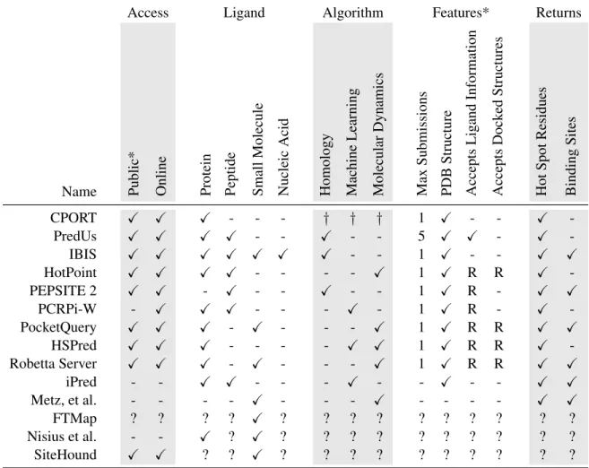
Table 1.2: Characteristics of existing algorithms for hot spot and binding site identification. * ’Public’ refers to unrestricted access of the software; R stands for required.
†CPORT returns a consensus from 6 different algorithms: WHISCY, PIER, ProMate, cons-PPISP, SPPIDER, and PINUP. These six, freely available packages are not detailed here as CPORT reported significantly improved
results even above the best of them.
proposed for hot spot identification (HSI) . The majority of HSI algorithms analyze protein surfaces for specific patterns of chemical and geometrical properties, such as charge, polarity, hydrophobicity, shape, or sequence [18, 27, 28, 29], while several recent algorithms utilize homology models to transitively identify binding sites [30, 31]. Table 1.2 provides a list of several popular algorithms.
must typically submit each protein or complex separately and wait several minutes to hours for the results. At the time of this writing, we are unaware of a publicly-accessible method that is capable of handling a large volume of queries. Most algorithms require that users sup-ply the protein or peptide ligand, and in some cases, the supplied ligand must already be in a native or native-like docking pose [26], further hindering the ability of these algorithms for discovering unknown PPIs. The reported prediction accuracy has not been high; few algo-rithms have reported a prediction accuracy above 60% [32]. Recent reviews commented on the difficulty of comparison between different approaches [6, 32] because each algorithm was tested and benchmarked on a different data set and validated with the different metrics. In general, homology-based algorithms have been shown to yield more accurate predictions, but by definition these are applicable only to proteins with known structural homologs[30, 32].
CHAPTER 2
Development of a SNAPP Scoring Function for Analysis of Protein Interactions
2.1 Creation of the SNAPP scoring function
The SNAPP scoring function was originally developed by the Tropsha laboratory in the late 1990s as a method to evaluate protein structure [33] and pioneered the use of a compu-tational geometry technique called Delaunay tessellation [34] for protein structure analysis1. Since its creation, SNAPP has been used to recognize protein folds [37], predict protein stabil-ity [38], simulate protein folding [39], identify structural motifs in protein folds [40], identify fold nuclei [41], distinguish between native and native-like versus decoy protein folds [41], and automate protein-function annotation [42]. The initial development of SNAPP has been summarized in a review [43].
2.1.1 Protein Representation
energy functions [44]. The goodness of a representation depends upon its application, and our coarse-grained representation emphasizes speed and stability over structural precision.
The SPPR representation of a protein employed by Singh et al. [33] originally used the Cα of each amino acid; however, Cαs were quickly replaced with the side-chain centroids,
including the Cα, for each residue. The use of side-chain centroids was found to be more
predictive [41] and results in a tessellation that is more stable against perturbation [45] when compared to the use of Cαs. Furthermore, each centroid is more robust against errors in
structural data versus an all atom model, where the loss of an atom may change the results of an energy calculation or predicted hydrogen bonding. A centroid minus an atom still retains the properties of its amino acid type but suffers a slight coordinate change. Although such a change could result in a modified Delaunay tessellation, a previous study found that Delaunay tessellation is sufficiently robust to handle centroid perturbations [45]. Centroid coordinates are less sensitive to side chain rotamers: Not only can the rotational movement be accounted for with a single translation, but the movement will be less drastic due to the constancy of the atoms that do not move. Even more importantly, side chain centroids lower the complexity of residue interactions from a multi-body to a single-body problem.
preserve structural information and allow for comparison between protein geometries [40, 43]. Figure 2.1A and B show an example of a tessellated protein
Tetrahedra are further classified by their residue composition and sequence adjacency (Fig-ure 2.1C), which simply means the types of residues involved and the peptide bonding between each of the residues. Although the exact distribution of tetrahedra is unique for each protein structure, the Tropsha group found that particular types of tetrahedra occur more often than statistically expected. This finding culminated in the SNAPP database and a novel, four-body statistical scoring function.
2.1.2 Calculating the SNAPP scoring function
The original SNAPP scoring function was defined by Singh, et al. [33] as follows: Given a training set of protein structures, all proteins are tessellated, and SNAPP scores are calculated for every possible simplex combination of amino acid composition and sequence adjacency according to the following equation:
qijkl = log
fijkl
pijkl
(2.1)
whereqis the SNAPP score for a simplex with amino acidsijkl; andfandpare the observed and expected frequencies of the simplex, respectively:
fijkl,t =
|sijkl|
|S| (2.2)
pijkl,t =Caiajakal (2.3)
where |S| is the cardinality of Delaunay simplices, s is a subset of all simplices S in the dataset, and ai is the observed frequency of amino acid i in the dataset. In the expected
probability p, C defines a combinatorial factor that accounts for redundancy of amino acid composition, e.g.,ijkl=jkli:
C = 4!
Qi
n|ai|
(2.4)
where n is the number of unique amino acids in the simplex, and |ai| is the cardinality of
amino acids of typei.
with products. Thus, once the SNAPP scores have been computed, calculating the SNAPP scoreQfor a new protein is simple: tessellate the protein; score each simplex according to its composition and sequence adjacency; and sum the individual SNAPP scores:
Q=Xqi (2.5)
2.2 Variations on a Theme
There have been three variations of the SNAPP methodology since its inception. Each follows the same basic structure given above, but includes slight modifications to refine and specialize the potential. These modifications include a filter on the scoring function output, slight changes to the scoring function itself, and alterations to the representation of the protein, which in turn alter the scoring function.
2.2.1 SNAPP and Protein Tertiary Structure
The first variation of SNAPP by Carter et al. [38] began as an attempt to approximate the free-energy difference,∆(∆G), of protein folding by evaluating native protein tertiary struc-ture using SNAPP. Carter et al. found that simplices composed of four hydrophobic residues occurred more frequently than expected by random chance, and proposed that these simplices encode information relevant to thermodynamically significant tertiary interactions. To test their hypothesis, Carter et al. selected five proteins with a total of seventy-six mutations with experimentally tested ∆G values. They identified core residues for each of the five proteins from either the literature or based on cumulative SNAPP scores greater than 1.5 ˚A, and gener-ated a series of variant proteins with single point mutations for each core residue. They found that the difference in SNAPP scores, ∆SNAPP, for hydrophobic simplices in the core of a protein correlated with experimental∆(∆G)values.
Addition-ally, the study introduced two changes to the SNAPP algorithm as set forth by Singh et al. First, Carter et al. focused on protein tertiary structure and therefore removed many simplices involving residues adjacent in the primary sequence as such simplices were said to be unin-volved in tertiary interactions. The second change was the removal of any simplices with a vertex-to-vertex edge distance greater than 10 ˚A on the basis that direct interactions will occur only at shorter distances. However, both of these changes were introduced as filters for the study rather than canonical changes to the SNAPP score.
One year later, Cammer et al. [40] introduced the first SNAPP variation in a study us-ing SNAPP to identify tertiary packus-ing motifs. This study expanded on the previous alter-ations, maintaining the 10 ˚A edge cutoff and explicitly stating the removal of all simplices except type 0 (Figure 2.1C), i.e., simplices without any sequence-adjacent residues. Cam-mer et al. used SNAPP to identify common sequence-structure motifs among simplices with similar residue composition. They found that simplices containing a balance of hydrophobic and polar residues occurred far more frequently than simplices with singular compositions. Furthermore, they found specific residue-sequence motifs for three separate protein families, suggesting that some of the motifs could be used as markers for protein functional families.
The SNAPP score variation introduced by Cammer et al. (referred to as SNAPP-Cammer) has been used in other studies [43, 48], but is typically reserved for evaluating tertiary inter-actions. In addition to the log-likelihood functions, the SNAPP-Cammer database contains a plethora of additional data for each type 0 simplex composition; however, many of the imple-mentation details have been lost, and exactly how this additional information was applied to the scoring function, if at all, is unknown. As a result, the SNAPP-Cammer scoring function used for comparison performs scores only type 0 simplices as described in the paper.
2.2.2 Predicting Native-like versus Decoy Structures
at-tempted to incorporate the sequence adjacency into the formula, along with redefining SNAPP as a multi-body contact energy:
Qαijkl=−kBT ln
fα ijkl
pijkl
(2.6)
whereαrepresents simplex type, and the observed frequencyf was redefined to
fijklα = |s
α ijkl|
|sα| (2.7)
where |s|is the cardinality of simplices in the dataset with a given type α and composition ijkl. Unfortunately, the inclusion of the type did not extend into the expected frequency
p. Gan et al. made a number of additional changes, including using a varied edge cutoff of
either 8 or 11 ˚A to allow for comparison of SNAPP scores created from datasets with fewer structures. The refined scoring was unsuccessfully used to select native-like conformations from a series of decoys.
Decoy discrimination still presented an inviting target for SNAPP, and Krishnamoorthy et al. [41] re-purposed SNAPP for the task. Like Gan et al. they saw the importance of including the simplex type, but Krishnamoorthy et al. also recalculated the expected simplex frequency:
pαijkl=Caiajakalpα (2.8)
wherepα is the frequency of type αtetrahedra in the dataset. Additionally, the −kBT term
mutations on protein stability and reactivity [49].
2.2.3 Accounting for Structural Variation
Protein structures obtained from X-ray crystallography or NMR can be imprecise: Exper-imental error and protein flexibility could lead to variation in the atomic coordinates, possibly resulting in a different Delaunay tessellation. In 2004, Bandyopadhay and Snoeyink [45] developed almost-Delaunay simplices to identify potential quadruplets that would occur if vertices within a point set were allowed small perturbations. Given a Delaunay tessellation, they identified possible Delaunay edges for all vertices within a minimum distance thresh-old of 10 ˚A and identified all possible simplices given these additional edges. Each of these simplices was said to be almost-Delaunayiff the simplex would be a Delaunay simplex after neighboring vertices were perturbed by a minimum distanceε≥0.
Bandyopadhyay and Snoeyink were able to visualize and quantify α-helices, β-sheets, and β-turns using Delaunay simplices; however, they also found that fewer almost-Delaunay simplices were created as proteins became increasingly structured and when side-chain centroids were used instead ofCαs. Additionally, they weighted the SNAPP potentials
based on the almost-Delaunay simplices and found that both versions were able to discrimi-nate native-like from decoy protein folding. Although almost-Delaunay is a unique and po-tentially useful technique for analysis of protein structure, we chose not to use it in this project due to the additional computational complexity and overhead required.
2.3 Modern Modifications (M2)
between the old and newer scoring functions. Second, we suspected that the expected simplex frequency used in the previous SNAPP iterations might be too simple to accurately portray the complexity of protein interactions; we set out to remodel the expected simplex frequency based on a multi-body chemical reaction. Third, we designed a set of novel cheminformatics-like descriptors to account for simplex features ignored by the SNAPP potentials.
2.3.1 The Current SNAPP Scoring Function
As a part of updating the SNAPP score, we needed to recompile the training sets. Un-fortunately, recompiling the training sets on PPI data meant that comparison against the old SNAPP-Bala potentials would not be accurate; we needed to recalculate a new set of SNAPP potentials on a set of single-chain proteins using the algorithm set for by Krishnamoorthy et al. We compiled a set of single-chain protein structures from the Richardson Top 500 [50], PICES [51], and a subset of the PDB [52], which we define in greater detail in Chapter 2.4.1. To help differentiate between other SNAPP scores, we refer to the updated potentials as SNAPP-Fold. The SNAPP-Fold potentials were created using the following equations, which include the simplex type. The SNAPP score for a single simplex qijkl,t with amino acids ijkl in
configuration typetis defined by:
qijkl,t = log
fijkl,t
pijkl,t
(2.9)
which, remains a log ratio of the observedf over the expectedpfrequencies. The frequencies f andphave likewise changed to account for the simplex type:
fijkl,t =
|sijkl,t|
|st|
(2.10)
pijkl,t =Caiajakalft (2.11)
iin the dataset, andftis the frequency of typetsimplices in the dataset:
ft =
|st|
|S| (2.12)
2.3.2 Redefining the Expected Frequency
When we first set out to redefine the SNAPP scoring function, our first concern was how the expected frequencypijkl,twas calculated. In all of the SNAPP variations, the expected
fre-quency estimates the likelihood that four particular residues will associate with each other due to random chance. We hypothesized that tetrahedral formation was not entirely due to random chance, but was constrained by the existing peptide bonds between sequential amino acids. To test our hypothesis, we designed three new expected frequencies based on (1) the distribution of Delaunay edges found in proteins, (2) the frequency of interaction between amino acids, as defined by Delaunay tessellation, and (3) the occupation frequency for cooperative binding.
Edge Frequency
Similar to the amino acid frequency ai used in the original SNAPP equation, the edge
frequency feij gives a ratio of the occurrence of an edge between residues of typeai andaj
across the dataset:
ai =
nai
Nresidues
(2.13) feij =
neij
Nedges
(2.14)
includes the simplex type:
pijkl= se Y
x
fex (2.15)
=
πpeptide(se) Y
x
fex
πnon−peptide(se) Y
y
fey (2.16)
whereseis the set of edges for a given simplex andΠpeptideis the projection of edgessethat
are peptide bonds. Like the original equation, we must also account for the redundancy of permutations due to amino acid and edge types:
pijkl =C σ(sE:t)
X
Πpeptide(se) Y
x
fex
Πnon−peptide(se) Y
y
fey (2.17)
whereσ(sE:t)is the selection of all possible edge permutations given a simplex of typet. The
final edge frequency serves as a basis for the other two scoring functions, substitutingfex for
the respective frequencies.
Interaction Frequency
Instead of using amino acid distributions alone to calculate likelihood potentials, we could consider the formation of a simplex similar to that of a chemical reaction in equilibrium:
A+B AB (2.18)
with a first order reaction raterand equilibrium coefficient ofK,
r=k1[A][B]−k2[AB] (2.19)
K = k1 k2
(2.20) = [AB]
where[A] is the concentration of A, and k1 and k2 are the rate coefficients. By treating the amino acid and edge distributions as the concentrations of each, we may approximate the frequency of interaction,fI, between two residues:
fI =
feij
faifaj
(2.22)
Occupation Frequency
The final potential builds upon the interaction frequency and approximates a cooperative binding frequencyfV that is loosely based on the Adair-Klotz equation [53], which gives the
fractional occupationv:
v =
Pn i i
Qi jKi[A]
j
1 +Pn
i
Qi
jKi[A]j
(2.23)
fV =
fei→jfej→ifaifaj
1 +fei→jfai +fej→ifaj
(2.24)
where the edge frequency has been given a directioni→jto indicateibinding to the structure beforej. Here, the directed edge frequency is substituted for the rate constant, and the amino acid frequency is substituted for the concentration. The occupation frequency ignores the higher order reactions: The values calculated for i > 1 were several orders of magnitude smaller and had little effect on the frequency.
Cheminformatics-like Descriptors for Simplices
com-pounds are described by numerical parameters called descriptors that encode its physical and chemical characteristics. These descriptors range from constitutional traits, such as the num-ber of atoms, to more complex topological indices, often based on the numnum-ber of bonds per atom, also known as the vertex degree. Descriptors are a core component of cheminformatics algorithms and are utilized to help predict experimental outcomes. In order to better evalu-ate the structural diversity of protein packing, we developed a series of (i) chemistry-based descriptors that describe inherent structural characteristics, (ii) geometry-based descriptors to characterize the three-dimensional conservation of residue quadruplets and (iii) topology-based using well-defined constitutional and topological indices (e.g., Kier & Hall, Randic) [54, 55]. A complete list of the calculated protein descriptors can be found in Appendix 5.32. Geometric descriptors characterize simplices by quantitatively scoring the conservation of their three-dimensional structure, such as volume, surface area, inter-residue distance and angles, tetrahedrality (i.e., a measure of deviance from an ideal tetrahedron) [33], and chirality. In particular, tetrahedral chirality uniquely characterizes protein structure by identifying not only nearest-neighbor residues but also their spatial orientation with one another. Because the underlying structure is always a tetrahedron, these data are quickly calculated and provide a simple comparison between tetrahedra with the same residue composition and sequence adjacency.
Topological descriptors aid in describing, discriminating, and qualitatively comparing PPI structure through graph theory, which is widely used in cheminformatics and has also been useful for studying protein structure [56, 57, 58], protein flexibility [59, 60], PPI structure [61], and protein-protein docking [62, 63]; however to our knowledge, we are the first group to apply graph theory to PPI described using Delaunay tessellation. Topological descriptors are quickly calculated and describe both connectivity and branching complexity, expressed as graph indices. Examples of graph indices include: the Wiener index, i.e., the length of the shortest path across a graph, which correlates to van der Waals surface area [64]; various
vertex centralities, e.g., vertex degree (Equation 2.25) and Eigenvector centrality (Equation 2.26), which measure the importance of a vertex within a graph:
¯ vi =
1
MPM
v=1vi
(2.25)
xi =
1
λPN
j Aijxj
, (2.26)
the Randic connectivity index (Equation 2.27), which expresses the level of graph branching [65]:
R=
X
all edges
(vi·vj)−
1
2, (2.27)
and the Estrada index (Equation 2.28), which characterizes protein folding [66]:
EE(G) =
n
X
i
eλi, (2.28)
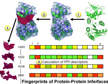
Descriptor calculation follows a simple workflow (Figure 2.2). First, each protein complex is subjected to Delaunay tessellation. Second, the calculation of these SNAP protein descrip-tors generates a series of numerical values for (a) each residue vertex, (b) each simplex, (c) each protein, and (d) special subsets of vertices, such as surface or interfacial residues. These numerical values specifically describe the constitutional, geometrical, and topological charac-teristics of each part of a protein, resulting in a protein fingerprint that can be used to analyze, sort, cluster, and model tetrahedra.
2.4 Validating the New Scoring Functions
Figure 2.2: Workflow to derive PPI fingerprints: (1) Tessellate a protein complex (PDB code 1A0O in this example); (2) Identify interfacial quadruplets; (3) Extract interfacial quadruplets; and (4) Calculate PPI descriptors (e.g., volume, exposed surface area, Kier & Hall indices).
of the six scoring functions to discriminate between native-like and decoy protein folds. We used SNAPP-Cammer, SNAPP-Bala, and with the newer SNAPP-Fold as controls to test the modified SNAPP potentials based on edge frequency, interaction frequency, and occupation frequency.
2.4.1 Compiling the Training Sets
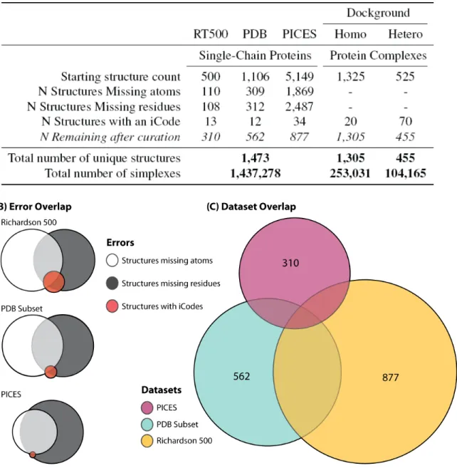
The selection and curation of the data used to create the scoring function directly relates to the algorithms efficacy and applicability. The databases used for training are summarized in Figure 2.3A, and the creation of the algorithm is described below.
and due to the low number of structures, we chose to add protein structures from additional sources. We selected a subset of single chain structures from the PDB with high resolution (<2 ˚A) and low sequence similarity (<35%) that contained only the protein itself, i.e., no ligands, co-factors, or nucleic acids. Further structures were added from PICES, a web server that ”culls” the PDB for structures according to R-factor.
All three training sets were curated, and any structures with one or more of the following problems were removed: missing atoms; missing entire residues; or containing an insertion code, or iCode (Figure 2.3B). The latter filter was chosen due to the inconsistent implementa-tion and poor quality of structures containing iCode data. Duplicate structures were removed with preference given to the Richardson dataset, followed by the PDB subset. Although the majority of each dataset was removed, the remaining datasets had surprisingly little overlap. The resulting database of 1,473 unique single-chain protein structures was tessellated and used to recompile the SNAPP scoring function (Figure 2.3C).
2.4.2 Benchmarking and comparison of new and old SNAPP scores
Two separate tests were used to validate the SNAPP scoring functions: (1) the Baker decoy set containing 60 protein backbones, i.e., only theCαs for each protein; and (2) the Rosetta
all-atom data set with 59 proteins [67].
The Baker decoy set [68] consists of sixty protein backbones, each with one native-like and three decoy structures. Each set of proteinCαs were tessellated and scored using
24 accurate predictions. When including predictions where the lowest RMSD had the second highest SNAPP score, Bala eked ahead with 38 correct predictions over SNAPP-Fold’s 36. Regardless, none of the scoring functions perform well, achieving little more than 60% native-like prediction accuracy for the dataset when the prediction standards are lowered. We hypothesize that some part of the poor predictions may likely be attributed to the use of Cαs for the protein structures rather than the side-chain centroids that SNAPP was trained
on. To validate this hypothesis, we decided to retest the SNAPP scoring functions using the Rosetta all-atom decoy set.
Figure 2.4: [Note to committee: This figure is confusing. I am fixing it and will send the updated figure.] The correlation between RMSD and SNAPP for the Baker decoy dataset. Proteins were put into one of four classes based on the SNAPP score rank of the lowest RMSD, e.g., if the highest scoring structure also has the lowest RMSD, it is put into class one. Shown are the percentages of proteins in each class as defined by the results from each of the three SNAPP scoring functions.
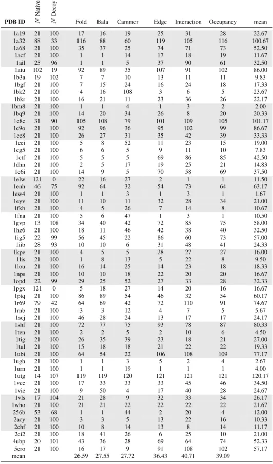
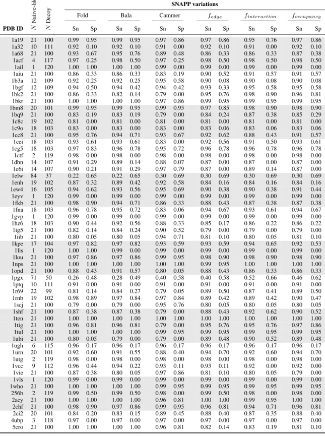
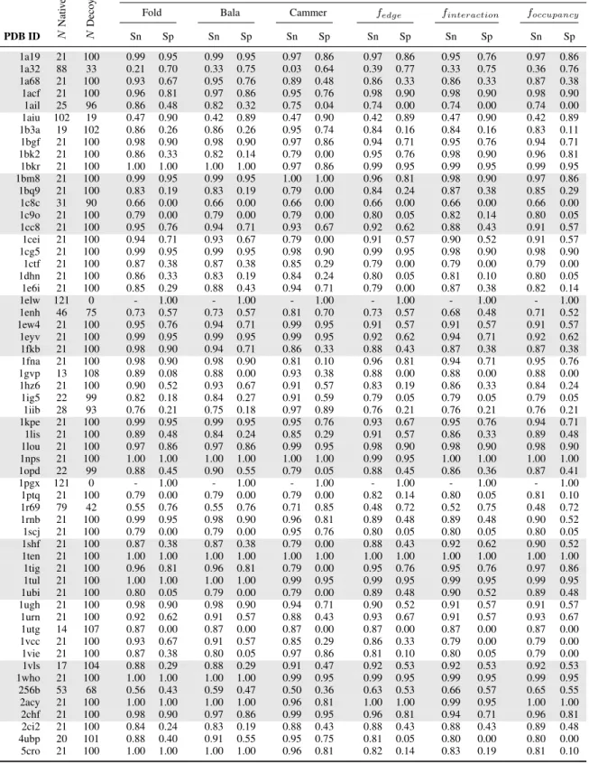
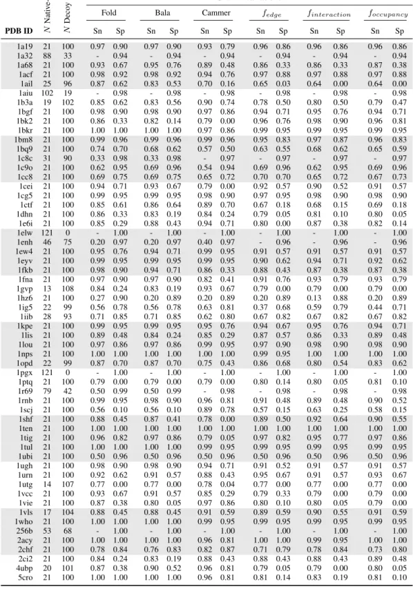
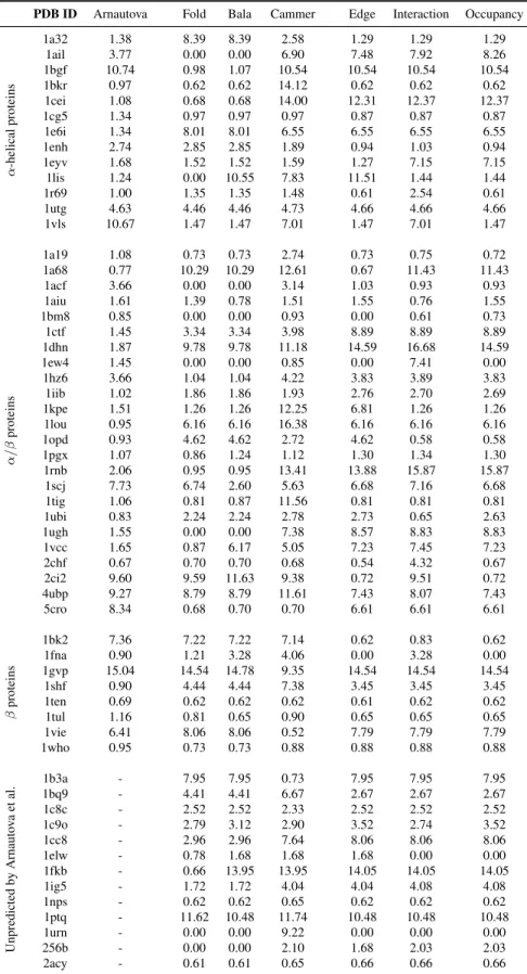
in a total of 121 structures per protein. For each protein group, we returned the rank of the native structure (Table 2.1), and calculated the sensitivity and specificity of the SNAPP scores based on the number of native and native-like structures as defined by an RMSD threshold of 1 ˚A (Table 2.2), 2 ˚A (Table 2.3), and 4 ˚A (Table 2.4). All of the SNAPP scores performed much better with the all-atom structures; however, SNAPP-Fold still outperformed the other scoring functions, followed closely by SNAPP-Bala, then by the Edge, Interaction, and Oc-cupancy frequencies, with SNAPP-Cammer trailing behind. In fact, for 43 of the 59 proteins, SNAPP-Fold scored the native protein within the top 10 highest scores of the other 121 in each set; of those 43 sets, the native was scored within the top 5 for 36 and as the highest scoring for 22 of the protein sets. Although none of the SNAPP scoring functions successfully found the native pose for more than 73% of the proteins, SNAPP-Fold consistently outperformed the other SNAPP variations, which unfortunately included the novel frequency variations.
We also compared our results for the Rosetta all-atom decoy set against those of Arnautova et al. [69]. Arnautova et al. developed three force fields for evaluating protein stability and tested their energy functions against 45 of the 59 proteins in the Rosetta all-atom decoy set. For each protein, their algorithm generated an additional 6,000 decoys to provide a smoother energy landscape for identifying the lowest energy conformation. They evaluated their scoring function based on the RMSD of the decoy with the lowest energy. The highest scoring protein found with SNAPP-Fold had a lower RMSD for 30 of the 45 protein sets, versus 26 and 17 for SNAPP-Bala and SNAPP-Cammer, respectively.
PDB ID N Nati v e-lik e N Deco y
Fold Bala Cammer Edge Interaction Occupancy mean
1a19 21 100 17 16 19 25 31 28 22.67
1a32 88 33 116 88 60 119 105 116 100.67
1a68 21 100 35 37 25 74 71 73 52.50
1acf 21 100 1 1 14 17 18 19 11.67
1ail 25 96 1 1 5 37 90 61 32.50
1aiu 102 19 92 89 35 107 91 102 86.00
1b3a 19 102 7 7 10 13 11 11 9.83
1bgf 21 100 7 15 24 16 24 18 17.33
1bk2 21 100 4 16 108 3 6 5 23.67
1bkr 21 100 16 21 11 23 36 26 22.17
1bm8 21 100 1 1 4 1 3 2 2.00
1bq9 21 100 14 20 34 26 8 20 20.33
1c8c 31 90 105 108 79 101 109 105 101.17
1c9o 21 100 92 96 36 95 102 99 86.67
1cc8 21 100 26 27 31 35 42 39 33.33
1cei 21 100 5 8 52 11 23 15 19.00
1cg5 21 100 6 6 5 9 11 10 7.83
1ctf 21 100 5 5 5 69 86 85 42.50
1dhn 21 100 2 5 17 19 25 21 14.83
1e6i 21 100 14 9 5 70 58 69 37.50
1elw 121 0 22 16 27 2 1 1 11.50
1enh 46 75 92 64 32 54 73 64 63.17
1ew4 21 100 1 1 3 1 3 1 1.67
1eyv 21 100 11 10 11 32 28 34 21.00
1fkb 21 100 4 5 26 7 14 8 10.67
1fna 21 100 5 6 47 1 3 1 10.50
1gvp 13 108 34 40 42 72 85 75 58.00
1hz6 21 100 18 11 46 42 38 40 32.50
1ig5 22 99 56 45 22 86 60 73 57.00
1iib 28 93 10 10 6 31 48 41 24.33
1kpe 21 100 4 5 5 28 27 27 16.00
1lis 21 100 1 8 13 5 22 8 9.50
1lou 21 100 16 14 25 14 23 18 18.33
1nps 21 100 10 10 18 22 20 20 16.67
1opd 22 99 29 25 52 27 33 28 32.33
1pgx 121 0 5 18 27 14 20 16 16.67
1ptq 21 100 86 89 54 46 32 54 60.17
1r69 79 42 64 69 42 72 110 91 74.67
1rnb 21 100 3 3 12 4 7 5 5.67
1scj 21 100 46 28 24 13 17 17 24.17
1shf 21 100 72 77 75 93 78 87 80.33
1ten 21 100 2 2 5 2 10 6 4.50
1tig 21 100 26 35 39 23 18 21 27.00
1tul 21 100 15 18 18 21 22 22 19.33
1ubi 21 100 64 54 22 106 108 109 77.17
1ugh 21 100 1 1 3 5 2 4 2.67
1urn 21 100 1 1 19 1 1 1 4.00
1utg 14 107 119 119 120 121 121 121 120.17
1vcc 21 100 17 33 33 33 45 46 34.50
1vie 21 100 9 50 4 17 40 28 24.67
1vls 17 104 21 28 9 32 33 34 26.17
1who 21 100 21 21 22 22 22 22 21.67
256b 53 68 1 1 44 2 20 4 12.00
2acy 21 100 3 3 5 13 22 16 10.33
2chf 21 100 10 8 14 13 8 14 11.17
2ci2 21 100 18 41 26 6 25 10 21.00
4ubp 20 101 43 36 28 69 64 74 52.33
5cro 21 100 16 17 9 91 108 102 57.17
mean 26.59 27.55 27.72 36.43 40.71 39.09
SNAPP variations
Fold Bala Cammer fedge finteraction foccupancy
PDB ID N
Nati v e-lik e N Deco y
Sn Sp Sn Sp Sn Sp Sn Sp Sn Sp Sn Sp
1a19 21 100 0.99 0.95 0.99 0.95 0.97 0.86 0.97 0.86 0.95 0.76 0.97 0.86
1a32 10 111 0.92 0.10 0.92 0.10 0.91 0.00 0.92 0.10 0.91 0.00 0.92 0.10
1a68 21 100 0.93 0.67 0.95 0.76 0.89 0.48 0.86 0.33 0.86 0.33 0.87 0.38
1acf 4 117 0.97 0.25 0.98 0.50 0.97 0.25 0.98 0.50 0.98 0.50 0.98 0.50
1ail 1 120 1.00 1.00 1.00 1.00 0.99 0.00 0.99 0.00 0.99 0.00 0.99 0.00
1aiu 21 100 0.86 0.33 0.86 0.33 0.83 0.19 0.90 0.52 0.91 0.57 0.91 0.57
1b3a 12 109 0.92 0.25 0.92 0.25 0.95 0.58 0.90 0.08 0.90 0.08 0.90 0.08
1bgf 12 109 0.94 0.50 0.94 0.42 0.94 0.42 0.93 0.33 0.95 0.58 0.95 0.58
1bk2 21 100 0.86 0.33 0.82 0.14 0.79 0.00 0.95 0.76 0.98 0.90 0.96 0.81
1bkr 21 100 1.00 1.00 1.00 1.00 0.97 0.86 0.99 0.95 0.99 0.95 0.99 0.95
1bm8 20 101 0.99 0.95 0.99 0.95 0.99 0.95 0.97 0.85 0.98 0.90 0.98 0.90
1bq9 21 100 0.83 0.19 0.83 0.19 0.79 0.00 0.84 0.24 0.87 0.38 0.85 0.29
1c8c 19 102 0.81 0.00 0.81 0.00 0.81 0.00 0.81 0.00 0.81 0.00 0.81 0.00
1c9o 18 103 0.83 0.00 0.83 0.00 0.83 0.00 0.83 0.06 0.83 0.06 0.83 0.06
1cc8 21 100 0.95 0.76 0.94 0.71 0.93 0.67 0.92 0.62 0.88 0.43 0.91 0.57
1cei 18 103 0.93 0.61 0.93 0.61 0.83 0.00 0.92 0.56 0.91 0.50 0.93 0.61
1cg5 18 103 0.97 0.83 0.96 0.78 0.95 0.72 0.96 0.78 0.96 0.78 0.96 0.78
1ctf 2 119 0.98 0.00 0.98 0.00 0.98 0.00 0.98 0.00 0.98 0.00 0.98 0.00
1dhn 14 107 0.91 0.29 0.89 0.14 0.88 0.07 0.87 0.00 0.87 0.00 0.87 0.00
1e6i 14 107 0.90 0.21 0.91 0.29 0.97 0.79 0.87 0.00 0.89 0.14 0.87 0.00
1elw 84 37 0.22 0.65 0.22 0.65 0.30 0.69 0.30 0.69 0.30 0.69 0.30 0.69
1enh 19 102 0.87 0.32 0.89 0.42 0.92 0.58 0.84 0.16 0.84 0.16 0.84 0.16
1ew4 16 105 0.94 0.62 0.93 0.56 0.95 0.69 0.90 0.38 0.90 0.38 0.91 0.44
1eyv 1 120 0.99 0.00 0.99 0.00 0.99 0.00 0.99 0.00 0.99 0.00 0.99 0.00
1fkb 21 100 0.98 0.90 0.94 0.71 0.86 0.33 0.88 0.43 0.87 0.38 0.87 0.38
1fna 18 103 0.96 0.78 0.95 0.72 0.83 0.06 0.94 0.67 0.93 0.61 0.94 0.67
1gvp 1 120 0.99 0.00 0.99 0.00 0.99 0.00 0.99 0.00 0.99 0.00 0.99 0.00
1hz6 18 103 0.90 0.44 0.92 0.56 0.88 0.33 0.85 0.17 0.86 0.22 0.86 0.22
1ig5 21 100 0.82 0.14 0.84 0.24 0.90 0.52 0.79 0.00 0.79 0.00 0.79 0.00
1iib 21 100 0.80 0.05 0.80 0.05 0.94 0.71 0.81 0.10 0.80 0.05 0.81 0.10
1kpe 17 104 0.97 0.82 0.97 0.82 0.93 0.59 0.93 0.59 0.94 0.65 0.92 0.53
1lis 1 120 1.00 1.00 0.99 0.00 0.99 0.00 0.99 0.00 0.99 0.00 0.99 0.00
1lou 21 100 0.97 0.86 0.97 0.86 0.99 0.95 0.98 0.90 0.98 0.90 0.98 0.90
1nps 21 100 1.00 1.00 1.00 1.00 1.00 1.00 0.99 0.95 1.00 1.00 1.00 1.00
1opd 21 100 0.88 0.43 0.91 0.57 0.80 0.05 0.88 0.43 0.86 0.33 0.86 0.33
1pgx 71 50 0.26 0.48 0.28 0.49 0.40 0.58 0.40 0.58 0.52 0.66 0.46 0.62
1ptq 10 111 0.91 0.00 0.91 0.00 0.91 0.00 0.91 0.00 0.91 0.00 0.91 0.00
1r69 22 99 0.81 0.14 0.84 0.27 0.79 0.05 0.89 0.50 0.87 0.41 0.89 0.50
1rnb 19 102 0.98 0.89 0.97 0.84 0.97 0.84 0.89 0.42 0.89 0.42 0.90 0.47
1scj 21 100 0.79 0.00 0.79 0.00 0.95 0.76 0.80 0.05 0.80 0.05 0.80 0.05
1shf 21 100 0.87 0.38 0.87 0.38 0.79 0.00 0.88 0.43 0.92 0.62 0.90 0.52
1ten 21 100 1.00 1.00 1.00 1.00 1.00 1.00 1.00 1.00 1.00 1.00 1.00 1.00
1tig 21 100 0.96 0.81 0.96 0.81 0.79 0.00 0.95 0.76 0.95 0.76 0.97 0.86
1tul 21 100 1.00 1.00 1.00 1.00 0.99 0.95 0.99 0.95 0.99 0.95 0.99 0.95
1ubi 21 100 0.80 0.05 0.79 0.00 0.79 0.00 0.89 0.48 0.90 0.52 0.89 0.48
1ugh 6 115 0.96 0.17 0.96 0.17 0.96 0.17 0.96 0.17 0.96 0.17 0.96 0.17
1urn 20 101 0.92 0.60 0.91 0.55 0.88 0.40 0.94 0.70 0.92 0.60 0.94 0.70
1utg 2 119 0.98 0.00 0.98 0.00 0.98 0.00 0.98 0.00 0.98 0.00 0.98 0.00
1vcc 9 112 0.96 0.44 0.94 0.22 0.93 0.11 0.93 0.11 0.92 0.00 0.92 0.00
1vie 21 100 0.87 0.38 0.80 0.05 0.97 0.86 0.81 0.10 0.80 0.05 0.79 0.00
1vls 1 120 0.99 0.00 0.99 0.00 0.99 0.00 0.99 0.00 0.99 0.00 0.99 0.00
1who 21 100 1.00 1.00 1.00 1.00 0.99 0.95 0.99 0.95 0.99 0.95 0.99 0.95
256b 2 119 0.99 0.50 0.99 0.50 0.98 0.00 0.99 0.50 0.98 0.00 0.98 0.00
2acy 21 100 1.00 1.00 1.00 1.00 0.96 0.81 1.00 1.00 0.99 0.95 1.00 1.00
2chf 21 100 0.98 0.90 0.97 0.86 0.99 0.95 0.96 0.81 0.94 0.71 0.96 0.81
2ci2 20 101 0.84 0.20 0.83 0.15 0.89 0.45 0.88 0.40 0.87 0.35 0.88 0.40
4ubp 3 118 0.97 0.00 0.97 0.00 0.97 0.00 0.97 0.00 0.97 0.00 0.97 0.00
5cro 21 100 1.00 1.00 1.00 1.00 0.96 0.81 0.82 0.14 0.83 0.19 0.81 0.10
SNAPP variations
Fold Bala Cammer fedge finteraction foccupancy
PDB ID N
Nati v e-lik e N Deco y
Sn Sp Sn Sp Sn Sp Sn Sp Sn Sp Sn Sp
1a19 21 100 0.99 0.95 0.99 0.95 0.97 0.86 0.97 0.86 0.95 0.76 0.97 0.86
1a32 88 33 0.21 0.70 0.33 0.75 0.03 0.64 0.39 0.77 0.33 0.75 0.36 0.76
1a68 21 100 0.93 0.67 0.95 0.76 0.89 0.48 0.86 0.33 0.86 0.33 0.87 0.38
1acf 21 100 0.96 0.81 0.97 0.86 0.95 0.76 0.98 0.90 0.98 0.90 0.98 0.90
1ail 25 96 0.86 0.48 0.82 0.32 0.75 0.04 0.74 0.00 0.74 0.00 0.74 0.00
1aiu 102 19 0.47 0.90 0.42 0.89 0.47 0.90 0.42 0.89 0.47 0.90 0.42 0.89
1b3a 19 102 0.86 0.26 0.86 0.26 0.95 0.74 0.84 0.16 0.84 0.16 0.83 0.11
1bgf 21 100 0.98 0.90 0.98 0.90 0.97 0.86 0.94 0.71 0.95 0.76 0.94 0.71
1bk2 21 100 0.86 0.33 0.82 0.14 0.79 0.00 0.95 0.76 0.98 0.90 0.96 0.81
1bkr 21 100 1.00 1.00 1.00 1.00 0.97 0.86 0.99 0.95 0.99 0.95 0.99 0.95
1bm8 21 100 0.99 0.95 0.99 0.95 1.00 1.00 0.96 0.81 0.98 0.90 0.97 0.86
1bq9 21 100 0.83 0.19 0.83 0.19 0.79 0.00 0.84 0.24 0.87 0.38 0.85 0.29
1c8c 31 90 0.66 0.00 0.66 0.00 0.66 0.00 0.66 0.00 0.66 0.00 0.66 0.00
1c9o 21 100 0.79 0.00 0.79 0.00 0.79 0.00 0.80 0.05 0.82 0.14 0.80 0.05
1cc8 21 100 0.95 0.76 0.94 0.71 0.93 0.67 0.92 0.62 0.88 0.43 0.91 0.57
1cei 21 100 0.94 0.71 0.93 0.67 0.79 0.00 0.91 0.57 0.90 0.52 0.91 0.57
1cg5 21 100 0.99 0.95 0.99 0.95 0.98 0.90 0.99 0.95 0.98 0.90 0.98 0.90
1ctf 21 100 0.87 0.38 0.87 0.38 0.85 0.29 0.79 0.00 0.79 0.00 0.79 0.00
1dhn 21 100 0.86 0.33 0.83 0.19 0.84 0.24 0.80 0.05 0.81 0.10 0.80 0.05
1e6i 21 100 0.85 0.29 0.88 0.43 0.94 0.71 0.79 0.00 0.87 0.38 0.82 0.14
1elw 121 0 - 1.00 - 1.00 - 1.00 - 1.00 - 1.00 - 1.00
1enh 46 75 0.73 0.57 0.73 0.57 0.81 0.70 0.73 0.57 0.68 0.48 0.71 0.52
1ew4 21 100 0.95 0.76 0.94 0.71 0.99 0.95 0.91 0.57 0.91 0.57 0.91 0.57
1eyv 21 100 0.99 0.95 0.99 0.95 0.99 0.95 0.92 0.62 0.94 0.71 0.92 0.62
1fkb 21 100 0.98 0.90 0.94 0.71 0.86 0.33 0.88 0.43 0.87 0.38 0.87 0.38
1fna 21 100 0.98 0.90 0.98 0.90 0.81 0.10 0.96 0.81 0.94 0.71 0.95 0.76
1gvp 13 108 0.89 0.08 0.88 0.00 0.93 0.38 0.88 0.00 0.88 0.00 0.88 0.00
1hz6 21 100 0.90 0.52 0.93 0.67 0.91 0.57 0.83 0.19 0.86 0.33 0.84 0.24
1ig5 22 99 0.82 0.18 0.84 0.27 0.91 0.59 0.79 0.05 0.79 0.05 0.79 0.05
1iib 28 93 0.76 0.21 0.75 0.18 0.97 0.89 0.76 0.21 0.76 0.21 0.76 0.21
1kpe 21 100 0.99 0.95 0.99 0.95 0.95 0.76 0.93 0.67 0.95 0.76 0.94 0.71
1lis 21 100 0.89 0.48 0.84 0.24 0.85 0.29 0.91 0.57 0.86 0.33 0.89 0.48
1lou 21 100 0.97 0.86 0.97 0.86 0.99 0.95 0.98 0.90 0.98 0.90 0.98 0.90
1nps 21 100 1.00 1.00 1.00 1.00 1.00 1.00 0.99 0.95 1.00 1.00 1.00 1.00
1opd 22 99 0.88 0.45 0.90 0.55 0.79 0.05 0.88 0.45 0.86 0.36 0.87 0.41
1pgx 121 0 - 1.00 - 1.00 - 1.00 - 1.00 - 1.00 - 1.00
1ptq 21 100 0.79 0.00 0.79 0.00 0.79 0.00 0.82 0.14 0.80 0.05 0.81 0.10
1r69 79 42 0.55 0.76 0.55 0.76 0.71 0.85 0.48 0.72 0.52 0.75 0.48 0.72
1rnb 21 100 0.99 0.95 0.98 0.90 0.96 0.81 0.89 0.48 0.89 0.48 0.90 0.52
1scj 21 100 0.79 0.00 0.79 0.00 0.95 0.76 0.80 0.05 0.80 0.05 0.80 0.05
1shf 21 100 0.87 0.38 0.87 0.38 0.79 0.00 0.88 0.43 0.92 0.62 0.90 0.52
1ten 21 100 1.00 1.00 1.00 1.00 1.00 1.00 1.00 1.00 1.00 1.00 1.00 1.00
1tig 21 100 0.96 0.81 0.96 0.81 0.79 0.00 0.95 0.76 0.95 0.76 0.97 0.86
1tul 21 100 1.00 1.00 1.00 1.00 0.99 0.95 0.99 0.95 0.99 0.95 0.99 0.95
1ubi 21 100 0.80 0.05 0.79 0.00 0.79 0.00 0.89 0.48 0.90 0.52 0.89 0.48
1ugh 21 100 0.98 0.90 0.98 0.90 0.94 0.71 0.90 0.52 0.91 0.57 0.91 0.57
1urn 21 100 0.92 0.62 0.91 0.57 0.88 0.43 0.93 0.67 0.91 0.57 0.93 0.67
1utg 14 107 0.87 0.00 0.87 0.00 0.87 0.00 0.87 0.00 0.87 0.00 0.87 0.00
1vcc 21 100 0.93 0.67 0.91 0.57 0.85 0.29 0.86 0.33 0.79 0.00 0.79 0.00
1vie 21 100 0.87 0.38 0.80 0.05 0.97 0.86 0.81 0.10 0.80 0.05 0.79 0.00
1vls 17 104 0.88 0.29 0.88 0.29 0.91 0.47 0.92 0.53 0.92 0.53 0.92 0.53
1who 21 100 1.00 1.00 1.00 1.00 0.99 0.95 0.99 0.95 0.99 0.95 0.99 0.95
256b 53 68 0.56 0.43 0.59 0.47 0.50 0.36 0.63 0.53 0.66 0.57 0.65 0.55
2acy 21 100 1.00 1.00 1.00 1.00 0.96 0.81 1.00 1.00 0.99 0.95 1.00 1.00
2chf 21 100 0.98 0.90 0.97 0.86 0.99 0.95 0.96 0.81 0.94 0.71 0.96 0.81
2ci2 21 100 0.84 0.24 0.83 0.19 0.88 0.43 0.88 0.43 0.88 0.43 0.89 0.48
4ubp 20 101 0.88 0.40 0.91 0.55 0.95 0.75 0.81 0.05 0.80 0.00 0.80 0.00
5cro 21 100 1.00 1.00 1.00 1.00 0.96 0.81 0.82 0.14 0.83 0.19 0.81 0.10
SNAPP variations
Fold Bala Cammer fedge finteraction foccupancy
PDB ID N
Nati v e-lik e N Deco y
Sn Sp Sn Sp Sn Sp Sn Sp Sn Sp Sn Sp
1a19 21 100 0.97 0.90 0.97 0.90 0.93 0.79 0.96 0.86 0.96 0.86 0.96 0.86
1a32 88 33 - 0.94 - 0.94 - 0.94 - 0.94 - 0.94 - 0.94
1a68 21 100 0.93 0.67 0.95 0.76 0.89 0.48 0.86 0.33 0.86 0.33 0.87 0.38
1acf 21 100 0.98 0.92 0.98 0.92 0.94 0.76 0.97 0.88 0.97 0.88 0.97 0.88
1ail 25 96 0.87 0.62 0.83 0.53 0.70 0.16 0.65 0.03 0.64 0.00 0.64 0.00
1aiu 102 19 - 0.98 - 0.98 - 0.98 - 0.98 - 0.98 - 0.98
1b3a 19 102 0.85 0.62 0.83 0.56 0.90 0.74 0.78 0.50 0.80 0.50 0.79 0.47
1bgf 21 100 0.98 0.90 0.98 0.90 0.97 0.86 0.94 0.71 0.95 0.76 0.94 0.71
1bk2 21 100 0.86 0.33 0.82 0.14 0.79 0.00 0.96 0.76 0.98 0.90 0.96 0.81
1bkr 21 100 1.00 1.00 1.00 1.00 0.97 0.86 0.99 0.95 0.99 0.95 0.99 0.95
1bm8 21 100 0.99 0.96 0.99 0.96 0.99 0.96 0.95 0.83 0.97 0.87 0.96 0.83
1bq9 21 100 0.74 0.70 0.68 0.62 0.57 0.50 0.63 0.55 0.68 0.62 0.65 0.59
1c8c 31 90 0.33 0.98 0.33 0.98 - 0.97 - 0.97 - 0.97 - 0.97
1c9o 21 100 0.62 0.95 0.69 0.96 0.54 0.94 0.69 0.96 0.62 0.95 0.69 0.96
1cc8 21 100 0.69 0.75 0.69 0.75 0.65 0.72 0.70 0.70 0.65 0.72 0.67 0.73
1cei 21 100 0.94 0.71 0.93 0.67 0.79 0.00 0.92 0.57 0.90 0.52 0.91 0.57
1cg5 21 100 0.99 0.95 0.99 0.95 0.98 0.90 0.97 0.95 0.98 0.90 0.98 0.90
1ctf 21 100 0.85 0.61 0.86 0.64 0.89 0.70 0.67 0.18 0.68 0.15 0.69 0.18
1dhn 21 100 0.86 0.33 0.83 0.19 0.84 0.24 0.79 0.05 0.81 0.10 0.80 0.05
1e6i 21 100 0.85 0.29 0.88 0.43 0.94 0.71 0.80 0.00 0.87 0.38 0.82 0.14
1elw 121 0 - 1.00 - 1.00 - 1.00 - 1.00 - 1.00 - 1.00
1enh 46 75 0.20 0.97 0.20 0.97 0.40 0.97 - 0.96 - 0.96 - 0.96
1ew4 21 100 0.95 0.76 0.94 0.71 0.99 0.95 0.91 0.57 0.91 0.57 0.91 0.57
1eyv 21 100 0.99 0.95 0.99 0.95 0.99 0.95 0.90 0.62 0.94 0.71 0.92 0.62
1fkb 21 100 0.98 0.90 0.94 0.71 0.86 0.33 0.88 0.43 0.87 0.38 0.87 0.38
1fna 21 100 0.97 0.90 0.97 0.90 0.82 0.41 0.91 0.76 0.93 0.79 0.93 0.79
1gvp 13 108 0.84 0.24 0.83 0.19 0.93 0.67 0.79 0.00 0.79 0.00 0.79 0.00
1hz6 21 100 0.27 0.90 0.20 0.89 0.20 0.89 0.20 0.89 0.13 0.88 0.20 0.89
1ig5 22 99 0.56 0.78 0.56 0.78 0.63 0.81 0.37 0.68 0.59 0.79 0.44 0.71
1iib 28 93 0.71 0.85 0.71 0.85 0.62 0.80 0.67 0.82 0.67 0.82 0.67 0.82
1kpe 21 100 0.99 0.95 0.99 0.95 0.95 0.76 0.94 0.67 0.95 0.76 0.94 0.71
1lis 21 100 0.89 0.48 0.84 0.24 0.85 0.29 0.87 0.57 0.86 0.33 0.89 0.48
1lou 21 100 0.97 0.86 0.97 0.86 0.99 0.95 0.97 0.90 0.98 0.90 0.98 0.90
1nps 21 100 1.00 1.00 1.00 1.00 1.00 1.00 0.99 0.95 1.00 1.00 1.00 1.00
1opd 22 99 0.87 0.70 0.87 0.70 0.75 0.43 0.86 0.68 0.80 0.54 0.83 0.62
1pgx 121 0 - 1.00 - 1.00 - 1.00 - 1.00 - 1.00 - 1.00
1ptq 21 100 0.79 0.00 0.79 0.00 0.79 0.00 0.80 0.14 0.80 0.05 0.81 0.10
1r69 79 42 0.50 0.99 0.50 0.99 - 0.98 - 0.98 - 0.98 - 0.98
1rnb 21 100 0.99 0.95 0.98 0.90 0.96 0.81 0.91 0.48 0.89 0.48 0.90 0.52
1scj 21 100 0.56 0.10 0.56 0.10 0.89 0.78 0.57 0.15 0.63 0.25 0.58 0.15
1shf 21 100 0.88 0.45 0.87 0.41 0.78 0.00 0.89 0.50 0.92 0.64 0.90 0.55
1ten 21 100 1.00 1.00 1.00 1.00 1.00 1.00 1.00 1.00 1.00 1.00 1.00 1.00
1tig 21 100 0.96 0.82 0.97 0.86 0.79 0.05 0.97 0.82 0.95 0.77 0.97 0.86
1tul 21 100 1.00 1.00 1.00 1.00 0.99 0.95 0.99 0.95 0.99 0.95 0.99 0.95
1ubi 21 100 0.50 0.96 0.50 0.96 0.50 0.96 0.50 0.96 0.50 0.96 0.50 0.96
1ugh 21 100 0.98 0.90 0.98 0.90 0.94 0.71 0.91 0.52 0.91 0.57 0.91 0.57
1urn 21 100 0.92 0.62 0.91 0.57 0.88 0.43 0.95 0.67 0.91 0.57 0.93 0.67
1utg 14 107 0.77 0.00 0.77 0.00 0.78 0.04 0.77 0.00 0.77 0.00 0.77 0.00
1vcc 21 100 0.93 0.67 0.91 0.57 0.85 0.29 0.79 0.33 0.79 0.00 0.79 0.00
1vie 21 100 0.87 0.38 0.80 0.05 0.97 0.86 0.80 0.10 0.80 0.05 0.79 0.00
1vls 17 104 0.88 0.45 0.88 0.45 0.91 0.59 0.89 0.59 0.90 0.55 0.91 0.59
1who 21 100 1.00 1.00 1.00 1.00 0.99 0.95 0.99 0.95 0.99 0.95 0.99 0.95
256b 53 68 - 1.00 - 1.00 - 1.00 - 1.00 - 1.00 - 1.00
2acy 21 100 1.00 1.00 1.00 1.00 0.96 0.81 1.00 1.00 0.99 0.95 1.00 1.00
2chf 21 100 0.78 0.84 0.76 0.83 0.82 0.87 0.71 0.79 0.78 0.84 0.73 0.80
2ci2 21 100 0.84 0.24 0.83 0.19 0.88 0.43 0.88 0.43 0.88 0.43 0.89 0.48
4ubp 20 101 0.87 0.38 0.90 0.52 0.96 0.81 0.79 0.05 0.79 0.00 0.80 0.05
5cro 21 100 1.00 1.00 1.00 1.00 0.96 0.81 0.81 0.14 0.83 0.19 0.81 0.10
PDB ID Arnautova Fold Bala Cammer Edge Interaction Occupancy
α
-helical
proteins
1a32 1.38 8.39 8.39 2.58 1.29 1.29 1.29
1ail 3.77 0.00 0.00 6.90 7.48 7.92 8.26
1bgf 10.74 0.98 1.07 10.54 10.54 10.54 10.54
1bkr 0.97 0.62 0.62 14.12 0.62 0.62 0.62
1cei 1.08 0.68 0.68 14.00 12.31 12.37 12.37
1cg5 1.34 0.97 0.97 0.97 0.87 0.87 0.87
1e6i 1.34 8.01 8.01 6.55 6.55 6.55 6.55
1enh 2.74 2.85 2.85 1.89 0.94 1.03 0.94
1eyv 1.68 1.52 1.52 1.59 1.27 7.15 7.15
1lis 1.24 0.00 10.55 7.83 11.51 1.44 1.44
1r69 1.00 1.35 1.35 1.48 0.61 2.54 0.61
1utg 4.63 4.46 4.46 4.73 4.66 4.66 4.66
1vls 10.67 1.47 1.47 7.01 1.47 7.01 1.47
α/β
proteins
1a19 1.08 0.73 0.73 2.74 0.73 0.75 0.72
1a68 0.77 10.29 10.29 12.61 0.67 11.43 11.43
1acf 3.66 0.00 0.00 3.14 1.03 0.93 0.93
1aiu 1.61 1.39 0.78 1.51 1.55 0.76 1.55
1bm8 0.85 0.00 0.00 0.93 0.00 0.61 0.73
1ctf 1.45 3.34 3.34 3.98 8.89 8.89 8.89
1dhn 1.87 9.78 9.78 11.18 14.59 16.68 14.59
1ew4 1.45 0.00 0.00 0.85 0.00 7.41 0.00
1hz6 3.66 1.04 1.04 4.22 3.83 3.89 3.83
1iib 1.02 1.86 1.86 1.93 2.76 2.70 2.69
1kpe 1.51 1.26 1.26 12.25 6.81 1.26 1.26
1lou 0.95 6.16 6.16 16.38 6.16 6.16 6.16
1opd 0.93 4.62 4.62 2.72 4.62 0.58 0.58
1pgx 1.07 0.86 1.24 1.12 1.30 1.34 1.30
1rnb 2.06 0.95 0.95 13.41 13.88 15.87 15.87
1scj 7.73 6.74 2.60 5.63 6.68 7.16 6.68
1tig 1.06 0.81 0.87 11.56 0.81 0.81 0.81
1ubi 0.83 2.24 2.24 2.78 2.73 0.65 2.63
1ugh 1.55 0.00 0.00 7.38 8.57 8.83 8.83
1vcc 1.65 0.87 6.17 5.05 7.23 7.45 7.23
2chf 0.67 0.70 0.70 0.68 0.54 4.32 0.67
2ci2 9.60 9.59 11.63 9.38 0.72 9.51 0.72
4ubp 9.27 8.79 8.79 11.61 7.43 8.07 7.43
5cro 8.34 0.68 0.70 0.70 6.61 6.61 6.61
β
proteins
1bk2 7.36 7.22 7.22 7.14 0.62 0.83 0.62
1fna 0.90 1.21 3.28 4.06 0.00 3.28 0.00
1gvp 15.04 14.54 14.78 9.35 14.54 14.54 14.54
1shf 0.90 4.44 4.44 7.38 3.45 3.45 3.45
1ten 0.69 0.62 0.62 0.62 0.61 0.62 0.62
1tul 1.16 0.81 0.65 0.90 0.65 0.65 0.65
1vie 6.41 8.06 8.06 0.52 7.79 7.79 7.79
1who 0.95 0.73 0.73 0.88 0.88 0.88 0.88
Unpredicted by Arnauto v a et al.
1b3a - 7.95 7.95 0.73 7.95 7.95 7.95
1bq9 - 4.41 4.41 6.67 2.67 2.67 2.67
1c8c - 2.52 2.52 2.33 2.52 2.52 2.52
1c9o - 2.79 3.12 2.90 3.52 2.74 3.52
1cc8 - 2.96 2.96 7.64 8.06 8.06 8.06
1elw - 0.78 1.68 1.68 1.68 0.00 0.00
1fkb - 0.66 13.95 13.95 14.05 14.05 14.05
1ig5 - 1.72 1.72 4.04 4.04 4.08 4.08
1nps - 0.62 0.62 0.65 0.62 0.62 0.62
1ptq - 11.62 10.48 11.74 10.48 10.48 10.48
1urn - 0.00 0.00 9.22 0.00 0.00 0.00
256b - 0.00 0.00 2.10 1.68 2.03 2.03
2acy - 0.61 0.61 0.65 0.66 0.66 0.66
of the published SNAPP variations provided exact details of the implementation method used to score tetrahedra and their proteins, and our implementation may have differed from that used in the literature. We suspect this is especially the case with SNAPP-Cammer.
Unfortunately, none of our frequency variations fared as well as Fold or SNAPP-Bala. In certain cases, the frequency variations performed exceptionally well when all other SNAPP potentials failed, but a quick glance did not reveal a prediction pattern for the fre-quency variations. We propose that a complete redesign of the SNAPP potentials using the frequency variations could improve decoy fold prediction; however, we leave that experiment for future studies.
Although we had hoped to see a cleaner discrimination between native-like and decoy folded protein structures, the purpose of testing against protein folding was not to improve decoy fold discrimination, but to compare our new SNAPP potentials against the existing variations. To this extent, the above experiments proved useful: We found that SNAPP-Fold consistently outperformed all other SNAPP potentials, and we will use SNAPP-Fold as a control when designing the SNAPP potentials for PPI.
2.4.3 Evaluation of SNAPP descriptors
To our knowledge, cheminformatics-like descriptors have not been previously applied to evaluate protein packing in relation to either protein folding or protein interactions. Without previous results or an established benchmark to compare against, we opted to forgo descrip-tor analysis on protein folding and instead focus on descripdescrip-tors for protein interactions. We calculated the novel SNAPP descriptors for docking decoys in the Dockground decoy dataset [70], which contains 61 different protein complexes, each with one native complex, one to twelve native-like complexes, and one hundred decoy poses. We define the target interface as the interface between the chains given by the dataset, and we tested to see if the SNAPP descriptors could discriminate between native-like and decoy complexes.
se-lected all interfacial simplices, which we define as simplices that contain vertices from both chains at the target interface. Descriptors were calculated for each simplex individually and applied to describe the interface as a whole, depending on the trait in question. For instance, the volume of an interface was calculated by adding the volumes of all participating simplices, whereas the surface area of an interface included only those triangular faces external to the interface, and tetrahedrality descriptors were averaged across all interfacial simplices. Any descriptors caught deserting were immediately put to the sword. Unfortunately, we found very little correlation across the entire dataset between any single or paired descriptor and the RMSD of the complex, although the descriptor-RMSD correlation varied from complex to complex. When we plotted the RMSD-descriptor points, we found that the native and native-like interfaces clustered somewhere along the y-axis while the decoys showed a u-shaped RMSD-descriptor correlation Figure 2.5, which is to say no correlation at all. For more than 60% of the protein complexes in the dataset, most of the native-like complexes were easily identifiable using one or more of the descriptors; however, the native complex often ended up buried beneath the native-like complexes and two or three high-RMSD decoys.
Figure 2.5: RMSD versus SNAPP Descriptors for porcine kallikrein A bound to bovine trypsin inhibitor (PDB code 2KAI). The red horizontal line in each graph shows the value of a de-scriptor for the native complex relative to the others. Despite the lack of a correlation with RMSD, three of the descriptors (the Randic and Weiner Indices and the interfacial surface area) were able to discriminate between most of the native-like and the decoy poses.
Figure 2.6: The distribution of descriptor values for 6,000 decoy poses for phospholipase A2 in complex with a synthetic pentapeptide (PDB code 1TKJ), ranked by RMSD. The left side of side of each graph also shows the RMSD for each pose as a green line and the descriptor value for the native complex is given as a red line. On the right, the linear fit is given as a red line.
2.5 Specializing for Protein Interactions
In cheminformatics, an Applicability Domain (AD) of a Quantitative Structure Activity Relationship (QSAR) model is the region of chemical space that is similar to compounds found in the training set for which a model is expected to yield accurate predictions [74, 75]. In the same manner, we must consider the AD for SNAPP; all previous versions of SNAPP were trained, tested and applied to single chain, folded protein structures and are potentially outside AD for PPI prediction. Ofran and Rost [76] quantified the difference between six types of protein-protein interactions, including two internal (intra-domain and domain-domain) and four external (homo-obligomers, homo-complexes, hetero-obligomers, hetero-complexes) in-teractions, and found different amino acid distributions and pairwise contacts for each of the six types. They found that the residue and contact differences between each of the six types of interfaces was in fact sufficient to quantitatively discriminate between the other interface types – even between the two internal interactions. With this in mind, we set out to define a new set of SNAPP potentials specifically designed to predict protein interactions.
2.5.1 Redesigning SNAPP for Protein Interactions
For this project, our goal is two-fold: (1) to predict where protein interactions occur, i.e., binding sites, on protein surfaces; and (2) predict and evaluate conformations of protein interactions. Although very similar, both problems require subtly different approaches. In addition, we further split each set of potentials based on the type of interface, i.e., from either a homo- or hetero-complex, used to train.
SNAPP for Binding Site Prediction
frequency f be the frequency of interfacial simplices found in a given dataset, and we let the expected frequency reflect the amino acids available to form interfacial simplices, i.e., surface residues. We redefined the amino acid frequencyaifrom Equation 2.11 to reflect the
frequency that a given amino acidiwill occur on the surface:
ai =
|Asurf ace(i)|
|Asurf ace|
(2.29)
where|Asurf ace(i)|is the number of times amino acid typeiis found on the surface of a protein
in the dataset versus all amino acids on the surface of all proteins of the dataset|Asurf ace|. The
new SNAPP-Surface potential reflects the likelihood that a simplex will form between two protein surfaces. However, a simplex formed from two separate protein chains cannot have four sequentially adjacent residues, and the type 4 tetrahedra (Figure 2.1C) will never occur. Fortunately, the potentials will naturally reflect this change, and no special cases need to be written into the algorithm.
SNAPP for Interface Prediction
To evaluate the likelihood of a given interface, we developed the SNAPP-Interface poten-tials. In the same manner as the SNAPP-Surface potentials, the SNAPP-Interface potentials redefine the data used to compute the observed frequencyf and expected frequency p. The observed frequency f also uses the interfacial simplices found in the dataset; however, the expected frequencypinstead uses the frequency of amino acids found at an interface:
ai =
|Ainterface(i)|
|Ainterface|
(2.30)
Homo- versus Hetero-complexes
further defined protein interactions as either obligatory, i.e. an obligomer, or transient, i.e., a complex. Obligatory interactions were defined as any interaction that typically lasted the life of the protein, such as the interaction between different chains of a hemoglobin molecule, whereas the transient interactions were temporary, such as that of an enzyme and substrate. Due to the small number of crystal structures, we differentiate only between homo- and hetero-complexes, resulting in a total of four SNAPP scoring functions specifically designed for analysis of protein interfaces: Surface:Homo, Surface:Hetero, SNAPP-Interface:Homo, and SNAPP-Interface:Hetero. A brief comparison between each of the five scoring functions is given in Table 2.6.
Trained On Tested On Used to Predict
SNAPP Version Single
Chain Proteins Homo-comple x es Hetero-comple x es Protein-Peptide Comple x es Single Chain Proteins Homo-comple x es Hetero-comple x es Protein-Peptide Comple x es Protein F olding Binding Sites Protein-Peptide Docking
Fold X X X X X X X
Surface:Homo X X X X X X
Surface:Hetero X X X X X X
Interface:Homo X X X X X
Interface:Hetero X X X X X
Table 2.6: A breakdown of the types of data each of the SNAPP scores was trained on and how they are applied.
2.5.2 Training Set – Dockground Database
in-teraction is listed as the same chain, and split the dataset into homo- and hetero-complexes. Each complex consisted of two or more protein chains; however, the dataset identifies a single target interface by specifying exactly two interacting chains. We decided to limit curation of the Dockground dataset to removal of PDBs containing an iCode due to two limiting factors: First, the use of only interfacial simplices yielded far less data with which to train the scoring functions, a full order of magnitude less than the equivalent amount of data for protein fold-ing. Second, residues on the surfaces of proteins typically assume multiple rotameric states, and as such, the side chain atoms may be missing atoms or absent entirely in the crystal struc-ture. The SNAPP-Surface:Homo and SNAPP-Surface:Hetero scoring functions are used in the CRACLe algorithm, and their evaluation will be discussed in the next chapter.
2.6 Conclusion
CHAPTER 3
Predicting Sites of Protein Interactions
In this chapter, we cover the development of the Critical Residue Analysis and Com-plementarity Likelihood (CRACLe) algorithm and software for identifying hot spot residues and binding sites. CRACLe has been developed as a rapid method for computational high-throughput screening of individual proteins to identify potential binding sites on the protein surface rather than a singular, time-consuming, high-resolution docking solution. We show that CRACLe is capable of correctly predicting binding sites in more than 85% of proteins from the PepX test set [78], 88% from the ZDock Bound test set [79], and 83% from the ZDock Unbound test set [79]. CRACLe is computationally efficient, capable of predicting binding sites for over 1,000 proteins in under seven minutes on a standard desktop computer versus PredUs [30], which required the same amount of time to run a single protein on its web server. This high-throughput prediction of putative protein-protein binding sites could enable building of protein interaction networks, provide an assessment of potential drug targets for peptide inhibitors, or provide a scoring filter in PPI decoy discrimination.
3.1 Materials and Methods
rep-resentative and highly curated dataset of 1,473 non-redundant single chain proteins from three independent databases. These SNAPP-Fold potentials outperformed previous SNAPP itera-tions in decoy discrimination on three independent datasets. Due to the difference in nature between internal protein folding and PPIs, we defined and compiled two novel SNAPP scor-ing functions called SNAPP-Surface and SNAPP-Interface that were trained on tessellated protein-protein interfaces for homo-complexes and hetero-complexes.
In this chapter, we focus on the SNAPP-Surface potentials. We used 1,448 and 540 protein complexes from the Dockground dataset to train two the new SNAPP-Surface scoring func-tions for evaluating protein surfaces, respectively called Surface:Homo and SNAPP-Surface:Hetero. Both of these scoring functions use the same equations given for SNAPP-Fold (Equation 2.9-2.12) with two important distinctions: First, the observed frequencyfincluded only simplices whose residues were found at protein-protein interfaces. Interfacial residues are commonly identified by their proximity to residues of their binding partners [80, 81]. Sim-ilarly, we defined interfacial residues based on the presence of a Delaunay edge, i.e., an edge defined by Delaunay tessellation, between the residues of interacting proteins. Second, the expected frequencyputilized only amino acid frequenciesaiof surface residues, i.e.,
solvent-exposed residues on protein surfaces. The use of surface residue frequencies was intended to enable SNAPP to discriminate between interfacial and non-interfacial surface residues rather than evaluating the likelihood of the interface itself.
3.1.1 Using Surface Residue Triplets to Identify Putative Binding Sites
![Figure 2.4: [Note to committee: This figure is confusing. I am fixing it and will send the updated figure.] The correlation between RMSD and SNAPP for the Baker decoy dataset.](https://thumb-us.123doks.com/thumbv2/123dok_us/8257676.2187809/36.918.237.740.448.781/figure-committee-confusing-fixing-updated-figure-correlation-dataset.webp)