F
UELP
RICEB
ELIEFS AND THEC
ONSUMERR
ESPONSE TOP
RICEF
LUCTUATIONS: T
HEC
HOICE BETWEENG
ASOLINE ANDD
IESELV
EHICLESBradley D. Shrago
A dissertation submitted to the faculty of the University of North Carolina at Chapel Hill in par-tial fulfillment of the requirements for the degree of Doctor of Philosophy in the Department of
Economics.
Chapel Hill 2017
Approved by:
Brian McManus
Gary Biglaiser
Jane Fruehwirth
Jonathan Williams
ABSTRACT
BRADLEY D. SHRAGO: Fuel Price Beliefs and the Consumer Response to Price Fluctuations: The Choice between Gasoline and Diesel Vehicles.
(Under the direction of Brian McManus)
ACKNOWLEDGMENTS
There are several individuals who significantly contributed to my progress as a graduate stu-dent, each of whose contributions to my personal and academic life were important in the devel-opment of this manuscript. First and foremost, I would like to thank my loving wife, Kayla, for managing the vast majority of our personal lives and efforts towards raising our children during the past six years. I will never forget the sacrifices she made to allow me to continue schooling into my late 20’s while working from home with our daughters and (begrudgingly) our dog, Ryder. I thank my two daughters Elodie and Paige, who for five and two years of my graduate studies offered me an outlet to enjoy time away from my work, whether this involved testing the transitiv-ity of their preferences or doing things which children actually enjoy.1 I thank my parents Andy
and Karen for motivating me to find modest enough academic success in high school to allow me to attend a college which allowed me to fulfill my potential, my brother Bryan for providing an academic role model at an impressionable age, and my brother Ben for teaching me that training in mathematics would have a greater impact on my future than training in ice hockey. I am grateful to my grandfather William Shrago and my late grandmother Florette Shrago for their contribu-tions to the education of myself and my father, and thankful for the sacrifices made by my late grandparents Albert Schneider and Marion Schneider Cullen to educate my mother. I thank all of my teachers who showed interest in my academic progress, particularly Mr. Senson and Ms. Pietruszka, the latter of whom unflinchingly believed a third-grader actually meant ‘zorilla’ and not ‘gorilla’. I thank my economics professors Jerry Savitsky, Santhi Hejeebu, and Todd Knoop as well as my mathematics professors Tony deLaubenfels, Steve Bean, and Ann Cannon for giving me exceptional training during my undergraduate years at Cornell College.
Many of the discussions I shared with my friends and colleagues I met in UNC’s graduate program were instrumental to my success. I thank all of my peers in my cohort who I worked
with during our first year who spent evenings doing problem sets in Gardner Hall, and those who contributed to joint projects in my second year. I am indebted to the participants in UNC’s Applied Microeconomics seminar series who offered me feedback over the past four years, and am partic-ularly grateful for the experience I gained while presenting my research. To my current coauthors Forrest Spence and Jeff Ackermann, I look forward to continuing to work together in the future. I am also grateful for feedback provided by Eddie Watkins, Quinton White, Julien Isnard, Ray Wang, Chunxiao Li, and Marcela Parada-Contzen during the biweekly UNC Empirical Industrial Organization meeting and the selflessness of Uyen Tran during the 2017 ASSA Annual Meeting in Chicago.
I sincerely thank my advisor, Brian McManus, who undertook the difficult task of develop-ing an aspirdevelop-ing Empirical Industrial Organization economist when he offered to advise me on my dissertation research. He made a continuous effort during my third and fourth years to keep me en-gaged in the literature, searching for research opportunities, and ultimately helping me to acquire my data and develop my proposal. Oftentimes in these early years, Brian undertook the uncom-fortable task of steering me away from research opportunities which would not have been fruitful, and tweaking my suggestions to lead me towards productive research topics. I am grateful for the efforts Brian put into helping me to finalize my job market paper during Summer 2016, and mo-tivating me to continue to improve my paper at times when I was struggling to continue doing so. His intense focus and thoughtful skepticism were necessary to instill within me the skills needed to conduct applied research, and critical to my own focus during my final year at UNC.
Donna Gilleskie and Helen Tauchen for their contributions to all of our graduate students, myself included, and Jeremy Petranka for offering support to my development as an instructor. Finally, I would like to remember the contributions of my former committee member Tiago Pires, who tragically passed away shortly before I defended my proposal. I was blessed with the opportu-nity to know Tiago during his three years as an Assistant Professor of Economics at UNC, and am indebted to him for the kindness, sincerity, and inquisitiveness with which he approached my work. Tiago was an extraordinary individual and an incredibly bright young economist, and I hope that should I ever stray from the example he set, I can refer back to these acknowledgments and remember the example he provided.
While I was on the job market during early 2017, I spent some time thinking about a list of questions which students had been asked in past interviews, one of which asked me to name three economists who I greatly admire. To an extent, answers to these questions are strategic. Should I simply name three highly respected researchers in my field? Would I be able to provide insight into who I am as a researcher by discussing the work of junior faculty which I have found valuable? While I’d gladly have discussed my admiration for the work of a variety of economists in my field, I know that an honest answer to the question could not be given without mentioning Tiago Pires. He was a bright and promising young economist who undoubtedly would have continued to develop his strong line of empirical research. His passion for academic research shone through in every aspect of our interactions, and his kindness and selflessness was instrumental to the success of myself and many of my fellow graduate students at UNC.
a few interactions during our seminar series. After asking whether we could meet and sending him a vague research proposal, he responded with a detailed list of comments and offered suggestions for literature which might offer insight into how I could frame the project. Our first meeting lasted somewhere around two hours, and through some bizarre string of events our conversation shifted from a discussion of empirical research on two-sided markets to an hour discussing the difficulties of properly specifying price beliefs in structural models of consumer behavior. While my work on two-sided markets and network effects was left for later, our discussion on price beliefs was instrumental in developing my dissertation.
TABLE OF CONTENTS
LIST OF TABLES . . . xi
LIST OF FIGURES . . . xiii
1 Introduction . . . 1
2 Literature Review . . . 7
2.1 The Consumer Response to Fuel Economy . . . 7
2.2 Automobile Fuel Choice . . . 9
2.3 The Elasticity of Demand for Gasoline . . . 10
2.4 Fuel Prices and Behavior of Heavy Vehicle Operators . . . 11
3 Data . . . 13
3.1 Vehicle Purchases . . . 13
3.1.1 Odometer Readings . . . 17
3.2 Fuel Prices . . . 18
3.3 Comparison of User-Generated Fuel Economy Data to EPA Measures . . . 21
4 Descriptive Analysis . . . 37
4.1 Descriptive Evidence: Fuel Choice . . . 37
4.2 Descriptive Evidence: Vehicle Miles Traveled . . . 40
5 Model . . . 45
5.1 Theoretical Model . . . 45
5.1.1 Second Period: VMT Decision . . . 46
5.2 Empirical Implementation . . . 48
5.2.1 Specifying Price Beliefs . . . 50
5.2.2 Likelihood Contributions . . . 51
5.2.3 Likelihood Contributions: Random Odometer Entry . . . 52
5.2.4 Selection Correction . . . 53
5.2.5 Identification . . . 56
6 Results . . . 61
6.1 Parameter Estimates . . . 61
6.2 Counterfactuals . . . 66
7 Conclusion . . . 78
A Appendix: Chapter 3 . . . 80
A.1 Institutional Details . . . 80
A.2 Data Cleaning . . . 83
A.2.1 Sample Extraction . . . 83
A.2.2 Aggregation Process . . . 85
A.3 Fuel Economy Drivetrain Adjustment . . . 87
A.4 Fuel Prices . . . 88
A.5 Stationarity of the Diesel Premium . . . 89
B Appendix: Chapter 4 . . . 98
C Appendix: Chapter 5 . . . 100
C.1 Theoretical Model . . . 100
D Appendix: Chapter 6 . . . 102
LIST OF TABLES
3.1 Market Shares (%), by Owner Type . . . 25
3.2 Selected Descriptive Statistics: All Registration Types . . . 26
3.3 Selected Descriptive Statistics: Personal Registrations . . . 26
3.4 Selected Characteristics of Pickup Truck Models . . . 27
3.5 Yearly Vehicle Miles Traveled . . . 28
3.6 Summary Statistics, by Length of Ownership . . . 29
3.7 Logit: Odometer Reading Dummy . . . 30
3.8 OLS Regressions of EPA Combined Fuel Economy on Self-Reported Measures . . 30
4.1 Logistic Regression of Fuel Choice in Heavy-Duty Trucks: All Registrations . . . 42
4.2 Logistic Regression of Fuel Choice in Heavy-Duty Trucks: Personal Registrations 43 4.3 OLS Regression of Log Yearly Mileage: Full Registration Sample . . . 43
4.4 OLS Regression of Log Yearly Mileage: Personal Registration Sample . . . 44
6.1 Estimates without Selection Correction . . . 70
6.2 Estimates with Selection Correction . . . 71
6.3 Estimates with Selection Correction and Random Coefficient . . . 72
6.4 Approximated Elasticities from 5% Fuel Price Change . . . 72
6.5 Observed vs. Simulated VMT Percentiles . . . 73
A.1 Missing Observations by Stage of Data Entry Algorithm by County . . . 91
A.2 Fuel Price Summary Statistics, by County . . . 92
A.3 United States Gasoline and Diesel Prices, by PADD . . . 93
A.4 Dickey-Fuller Test Results: United States . . . 93
A.5 Dickey-Fuller Test Results: Rocky Mountain Region . . . 93
B.1 OLS Regression of Log Yearly Mileage: Business Registration Sample . . . 98
B.2 Logistic Regression of Fuel Choice in Heavy-Duty Trucks: Business Registrations 99
D.1 Multinomial Logit Estimates . . . 103
LIST OF FIGURES
3.1 Lognormal Fit of Diesel VMT Distribution . . . 31
3.2 Comparison of Gasoline and Diesel VMT Distributions . . . 31
3.3 Topographical Map of Washington with Oil Distribution Network . . . 32
3.4 Price Difference between Gasoline and Diesel, 01/01/2012-12/31/2015 . . . 33
3.5 Gasoline Price, 01/01/2012-12/31/2015 . . . 33
3.6 Diesel Price, 01/01/2012-12/31/2015 . . . 34
3.7 Example of Savings from Diesel Engine Upgrade . . . 34
3.8 Screenshot of Fuelly Interface . . . 35
3.9 Differences between Self-Reported and EPA Fuel Economy Estimates . . . 35
3.10 Scatterplot of Self-Reported and EPA Measures (A) . . . 36
3.11 Scatterplot of Self-Reported and EPA Measures (B) . . . 36
5.1 Cross-Sectional Identifying Variation with Kernel Density Estimate . . . 60
5.2 Time-Series Identifying Variation . . . 60
6.1 Counterfactual Fleet Fuel Economy . . . 73
6.2 Counterfactual Change in Fleet Fuel Economy . . . 74
6.3 Counterfactual Change in Mean VMT . . . 74
6.4 Counterfactual Average Fuel Consumption . . . 75
6.5 Counterfactual Change in Fuel Consumption . . . 75
6.6 Observed and Simulated VMT Distribution for SampleN1 . . . 76
6.7 Counterfactual VMT Distribution, Full Sample . . . 76
6.8 Counterfactual Mean VMT With/Without Selection Adjustment . . . 77
A.1 Count of Retailers Reporting Fuel Prices . . . 94
A.3 Count of Daily Gasoline Price Reports, by Filling Station . . . 95
A.4 U.S. Diesel Premium, 1994-2016 . . . 96
A.5 Rocky Mountain Region Diesel Premium, 1994-2016 . . . 96
A.6 West Coast Region Diesel Premium, 1994-2016 . . . 97
D.1 Simulated VMT Distribution, by Subsample . . . 105
D.2 Counterfactual VMT Distribution, by Subsample . . . 105
D.3 Comparison of Results Across Specifications: Fleet Fuel Economy . . . 106
D.4 Comparison of Results Across Specifications: Vehicle Miles Traveled . . . 106
D.5 Comparison of Results Across Specifications: Fuel Consumption . . . 107
D.6 Counterfactual Fleet Fuel Economy (A) . . . 107
D.7 Counterfactual Change in Fleet Fuel Economy (A) . . . 108
D.8 Counterfactual Change in Mean VMT (A) . . . 108
D.9 Counterfactual Average Fuel Consumption (A) . . . 109
D.10 Counterfactual Change in Fuel Consumption (A) . . . 109
D.11 Counterfactual Fleet Fuel Economy (B) . . . 110
D.12 Counterfactual Change in Fleet Fuel Economy (B) . . . 110
D.13 Counterfactual Change in Mean VMT (B) . . . 111
D.14 Counterfactual Average Fuel Consumption (B) . . . 111
SECTION 1
INTRODUCTION
Understanding consumers’ responsiveness to fuel prices and their willingness to substitute into non-gasoline powered engines carries significant importance to both environmental and economic policy. In the United States, the transportation sector accounts for roughly one fourth of green-house gas emissions, the majority of which can be attributed to usage of petroleum-based fuels in automobiles and trucks. Overall, energy expenditures have typically represented between 5% and 10% of GDP over the past few decades. In recent years, a variety of policy mechanisms have been proposed and implemented in hopes of reducing environmental damages and reliance on foreign energy sources. Broadly speaking, policy goals tend to be aimed at reducing per-mile fuel consumption from gasoline and diesel-powered engines as well as incentivizing development and adoption of vehicles which operate on renewable fuels.1 Despite the recent attention to
non-gasoline fleet development and recent growth in availability of electric and diesel-powered cars, market shares of non-gasoline powered cars, SUVs, and vans remain low throughout the United States. This poses a challenge for researchers studying fuel choice among U.S. automobile pur-chasers, as fuel choice has not been a matter of serious consideration for the vast majority of car, SUV, and van purchasers for much of the last century.
In this paper, I consider the market for pickup trucks as a means to study the role of price expectations and heterogeneity in expected use on fuel choice, fuel economy, and subsequent us-age decisions. My decision to focus on this market is based on the limited availability and low
1Examples of such policies include federal and state-level purchase subsidies for electric vehicles, subsidies at the
adoption rates of non-gasoline vehicles in the United States, as the market for pickup trucks is the only segment of the U.S. automobile market where (i) vehicles powered by different fuels have significant market shares and (ii) a large share of vehicles is purchased by individuals rather than fleet managers.2 I employ a rich dataset of vehicle registrations and high-frequency retailer-level fuel prices in the state of Washington from 2012-2015. My fuel price data, along with the presence of odometer readings attached to a subset of vehicle observations, allows me to account for two econometric challenges facing researchers who study fuel choice: modeling price expectations in a manner consistent with the beliefs of vehicle purchasers, and accounting for the role of selection into fuel type on anticipated usage.
The issue of selection on anticipated usage is well-documented in the literature and summa-rized by Bento et al. (2011), who show that the energy paradox in fuel economy could be partly explained by unobserved heterogeneity in usage intensity.3 Selection on anticipated usage is an im-portant consideration for fuel choice in the pickup truck market as well. In this market, the diesel engine option is a costly upgrade (typically several thousand dollars) available on large trucks as a means to reduce operating costs and improve performance.4 Thus, one might suspect that those
individuals with a high level of anticipated usage should have a greater willingness to pay for the engine’s attributes, and in turn be more likely to select the upgrade. In order to account for se-lection on anticipated usage, I use a two-period model of product choice and subsequent usage following Einav et al. (2013) and Gillingham (2013). In my specification, individuals’ expected utility from operating the vehicle is scaled by a parameter which represents their usage type at the point of vehicle purchase. For those individuals with a high level of expected usage, it is more
2Based on vehicle registration data provided to me by the Washington Department of Licensing (DOL), roughly
one fifth of new, personally-registered pickup trucks purchased from 2012-2015 in the state run on diesel, with all but a few dozen of the remaining vehicles operating on gasoline.
3The energy paradox refers to the phenomenon wherein individuals seemingly undervalue the present discounted
value of energy savings when making purchases.
4Until the 2014 model year, the diesel engine had only been available on heavy-duty pickup trucks. Dodge began
likely that the utility gains associated with adoption of the more efficient, high-performance diesel engine will outweigh the upgrade cost. By employing odometer readings for a subset of my vehicle registrations, I am able to identify the distribution of usage types and allow adoption decisions to shift based on individuals’ anticipated usage levels.
Within any model of vehicle choice the researcher must consider consumers’ formation of fuel price beliefs over the life-cycle of the vehicle. Forecasting gasoline and oil prices is a rich liter-ature unto itself, and there is a plethora of studies which attempt to improve upon a no-change forecast, where the expected price of gasoline at any point in the future is equivalent to its current price.5 Alquist et al. (2011) summarize the predictive power of a variety of methods of forecasting oil prices, and find limited evidence of models which offer a forecast improvement over the no-change forecasting model. This evidence is consistent with consumers’ elicited beliefs from sur-veys as well. Anderson et al. (2013) find that after controlling for inflation expectations, long-term household gasoline price expectations can be reasonably approximated by a no-change forecast. Given this evidence, prior researchers have often specified a no-change forecast for gasoline prices when modeling vehicle adoption, an approach which I also follow for gasoline prices.
The decision of whether to upgrade to a diesel engine requires consumers to forecast operating costs, relative to the engine’s gasoline counterpart, over the vehicle’s life. While gasoline price beliefs may be reasonably approximated by a no-change forecast, this need not hold for the price differential between the two fuels (referred to as the ‘diesel premium’ below). In Washington, variation in the diesel premium consists of both geographic price variation which is relatively persistent, as well as time-series variation which exhibits mean-reversion.6 This suggests that
the price beliefs of a forward-looking individual may respond differently to different sources of variation in the diesel premium.7 As a result, a no-change forecast of the diesel premium over the
5I use the term no-change forecast to refer to the family of price forecasts where the forecast price in the future is
today’s price. As such, a random walk price forecast fits into this family.
6In§A.5, I document the mean-reverting nature of the diesel premium.
7Li et al. (2014) document that consumers exhibit a stronger response to variation in gasoline taxes than to other
life of a vehicle may be improved upon by forecasting the diesel premium based on the historical average in the individual’s locale rather the current diesel premium.
My model of vehicle adoption and subsequent usage offers the opportunity to endow individ-uals with a variety of price beliefs. Considering the mean-reverting nature of the diesel premium, one approach is to specify expectations based on the average diesel premium in an individual’s lo-cale, and assume that individuals’ diesel price forecasts fully account for mean-reversion. An alter-native approach is to consider the possibility that individuals do not recognize the mean-reverting nature of the diesel premium and assume the same no-change forecast used for gasoline prices is applied to the diesel premium. A third possibility is that neither of these approaches are consistent with individuals’ price beliefs, and that individuals’ price beliefs do change in response to mean-reverting variation in the diesel premium, but to a lesser extent than the no-change forecast would imply. Rather than making an ex-ante assumption regarding which of the three possibilities repre-sents consumers’ price beliefs, I specify price expectations such that a parameter to be identified sheds light on which beliefs are most consistent with consumer behavior.
Identifying the type of price beliefs most consistent with consumer behavior within the confines of my model requires me to separately identify consumers’ responsiveness to time-series variation in the diesel premium from other sources of fuel price variation which consumers may perceive as more likely to persist throughout the life of a vehicle. This can be accomplished because of the atypically high level of cross-sectional variation in both gasoline prices and the diesel premium within the state of Washington. Whereas the western portion of the state receives fuel primarily from West Coast fuel transportation networks, the eastern portion of the state receives fuel pri-marily from the Rocky Mountain region’s fuel transportation networks. There is no pipeline which crosses the Cascade mountains, which bisect the state from north to south. Transporting fuel across the state is costly as it must either be done via roadways or marine transport via the Columbia River (EIA, 2015). As a result, gasoline prices tend to be higher and the diesel premium lower to the west of the Cascades relative to prices to the east of the Cascades. Persistently higher levels of
gas prices and a lower diesel premium result in considerably larger operating cost savings from upgrading to a diesel engine. In terms of the lifetime operating cost differential between a gasoline and diesel powered variant of a particular truck, such cross-sectional variation in fuel prices results in thousands of dollars of variation in savings associated with the diesel option. Given that my data contain upwards of 90,000 new truck purchases across the state, this cross-sectional variation in fuel prices allows me to identify consumers’ responsiveness to a relatively persistent source of variation in the diesel premium. Given consumers’ responsiveness to this source of price variation, the extent to which consumers respond to time-series variation in the diesel premium allows me to identify a crucial parameter attached to price beliefs.
Although the specific nature of the diesel premium’s transitory time-series variation need not apply in other settings, this treatment of price expectations embedded in a structural model of vehicle adoption can be employed in any situation where a no-change forecast may not represent a reasonable proxy for price beliefs, given the proper identifying variation. For example, in the case of electric vehicles, one might surmise based on increasing deployment of charging stations that individuals forecast the operating cost of an electric vehicle to decrease over the vehicle’s life-cycle. With adequate variation in both (i) installed charger bases at the time of purchase and (ii) rates of charger deployment across locations, one could estimate the importance of both current charging infrastructure as well as expectations over future infrastructure.
SECTION 2
LITERATURE REVIEW
The automotive industry is one of the largest in the United States and has been studied ex-tensively by economists over the past century. An early literature review on the industry was conducted by Griffin (1928), and it has continued to garner interest from economists over the past century. As such, I limit my review to the areas of literature to which this project most directly contributes. The primary contribution of this project lies at the intersection between two related but largely separate branches of research, as I study the consumer response to fuel economy in an environment where multiple fuels enjoy a significant market share. This paper makes a direct contribution to the literature on the consumer response to fuel price fluctuations as well as the liter-ature on fuel choice. In addition to the primary contributions made across these two branches, the findings in this project also have relevance for the literature on fuel taxation as well as an emerg-ing literature which considers the adoption of larger vehicles, a product class which has garnered limited interest in earlier work on the consumer response to fuel price fluctuations.
2.1 The Consumer Response to Fuel Economy
scrappage decisions of efficient versus inefficient vehicles. In a paper which is methodologically similar to mine, Gillingham (2013) considers the importance of selection into fuel efficient vehicles on anticipated usage when estimating the elasticity of fleet fuel economy. Using data on odometer readings from California’s smog check programs, he is able to model selection on anticipated usage and estimates the elasticity of the new vehicle fleet’s fuel economy as 0.09. Klier and Linn (2010) exploit a thirty-year panel of fuel prices and vehicle sales and estimate an elasticity of new vehicle fleet fuel economy of 0.12, whereas Austin and Dinan (2005) produce an estimate of 0.22 in a paper which includes a supply-side model of the automobile industry. Gramlich (2009) likewise incorporates a supply-side model where manufacturers can respond to fuel price fluctuations by selecting the fuel economy of their automobiles, and also produces estimates suggestive of a higher elasticity than those papers which do not include a supply-side model.
2.2 Automobile Fuel Choice
Owing to the dominance of gasoline-powered automobiles in the U.S. and the fact that avail-ability of vehicles with multiple fuel offerings was limited until recent years, the literature on fuel choice in the U.S. automobile market is somewhat limited. Early research studying fuel choice in the U.S. market, such as Brownstone et al. (1996, 2000) and Brownstone and Train (1999), relies in part on stated preference data over hypothetical alternative-fuel vehicles due to the absence of available alternative-fuel vehicles. More recently, researchers have considered the role of network effects and purchase subsidies on the adoption of newer alternative-fuel technologies. Corts (2010) and Shriver (2015) study the impact of flex-fuel vehicle adoption on the subsequent development of E85 retail infrastructure, and estimate that adoption of flex-fuel vehicles increases the number of local fuel retailers offering E85 fuel. However, the market for these vehicles differs from many alternative-fuel adoption choices as the fuel choices made by drivers of flex-fuel vehicles are made at the pump rather than at the point of vehicle purchase. Further, evidence indicates that even among those who do own a flex-fuel vehicle, the fuel is not widely used (Anderson and Sallee, 2011). The role of network effects and purchase subsidies in electric vehicle (EV) adoption is considered by Li et al. (2015), while Holland et al. (2015) document the importance of regional heterogeneity in environmental impacts associated with EV adoption when determining optimal purchase subsidies.
In countries where the penetration of non-gasoline powered personal vehicles is more signif-icant, consumers often do face a fuel choice in automobile adoption. As such, there is a larger literature considering the impact of fuel prices on fuel choice outside of the U.S. market. Yeh (2007) considers various policies which may drive cross-country differentials in natural gas vehi-cle adoption, estimating that the price of natural gas would need to be roughly 50% cheaper than gasoline or diesel to lead to widespread adoption in the U.S.1 The choice between gasoline and
diesel vehicles has been studied by Verboven (2002) and Linn (2014). Verboven (2002) studies
1Historically, natural gas is only about 20% cheaper than gasoline and diesel. Many personal vehicles in the U.S.
quality-based price discrimination in the European automobile market by considering consumers’ choices over gasoline and diesel engines. Verboven’s work differs from mine for a few reasons. Most importantly, Verboven’s work is aimed towards studying price discrimination, where the more efficient diesel engines represent a higher quality variant of the vehicle. While fuel prices enter the model of engine choice, he does not aim to identify the impact of separate sources of price variation or explicitly model price beliefs. Whereas my work relies on both time-series and cross-sectional variation in the incentives to adopt a diesel engine as a means to identify responses to these different types of price variation, Verboven relies on cross-sectional policy differences between different nations to identify consumers’ preferences over fuel efficiency. Linn (2014) considers the determinants of cross-country variation in diesel adoption rates, and finds evidence that underlying heterogeneity in consumer preferences over fuel economy explains a significant share of the variation.
2.3 The Elasticity of Demand for Gasoline
There is a rich literature built around estimating the price elasticity of demand for gasoline, owing to the importance of gasoline consumption to climate change, energy security, and its role in the production process of a wide variety of firms. While my work allows me specifically to produce estimates of the elasticity of fuel consumption for pickup truck drivers, it is worthwhile to be aware of broader estimates of this demand elasticity. Espey (1998) conducts a meta-analysis of the elasticity of gasoline demand which acts to summarize studies conducted between 1966 and 1997. She documents a median estimate of -0.23 for the short-run elasticity and a median estimate of -0.43 for the long-run elasticity of demand for gasoline. Recent literature, however, suggests that the demand for gasoline has become more inelastic since the turn of the millennium. Hughes et al. (2008) estimate that whereas the short-run price elasticity of gasoline demand lay between -0.21 and -0.34 between 1975 to 1980, this price elasticity had fallen to an estimated range between -0.03 and -0.08 between 2001 and 2006.
document a declining rebound effect, wherein individuals who purchase more energy-efficient products increase their utilization. Over the course of a thirty-five year panel spanning 1966-2001, they estimate a short-run (long-run) rebound effect of 0.045 (0.222). Estimates from this paper using the higher real income levels and lower real gasoline prices towards the end of the sample yield estimates roughly half the size of their estimates from the full period, again suggesting the consumer response has moderated in recent years. Whereas the rebound effect measures the impact of a decrease in operating costs on driving behavior resulting from higher fuel efficiency, other work considers the impact of decreased operating costs on driving behavior which results from lower gasoline prices. Linn (2013) documents that the magnitude can differ significantly, as he estimates an elasticity of vehicle miles traveled with respect to gasoline prices between -0.09 and -0.20 whereas he estimates a rebound effect between 0.20 and 0.40. In addition to producing an estimate of the elasticity of fleet fuel economy, Gillingham (2013) estimates the elasticity of demand for driving as -0.15 among a large sample of California drivers, whereas Gillingham (2014) produces a demand elasticity of -0.22 while also documenting significant heterogeneity in the elasticity across various demographics.
2.4 Fuel Prices and Behavior of Heavy Vehicle Operators
measures from the Vehicle Use and Inventory Survey.2 However, the age of the data, which were
last collected in 2002, limits its applicability to future studies in this area. A case-study approach is taken by Klemich et al. (2014) to study the energy paradox among motor carriers. They document a significant use of a wide variety of fuel saving tactics by motor carriers, and offer a discussion of the determinants for whether particular technologies were adopted. One of the most significant challenges in this area is limited publicavailability of data regarding fuel economy and vehicle usage, and while my work does not directly contribute to this line of research on commercial vehicles usage, my use of user-generated data on fuel economy could be of interest to researchers looking to further explore this topic.
2Leard et al. do not consider pickup trucks due to the limited sample observed in their micro-data. Therefore,
SECTION 3
DATA
Throughout this project, I use two primary datasets which I appended with data from additional sources. The Washington Department of Licensing (DOL) provides a database of all vehicle trans-actions within the state of Washington from January 1 2012 through December 31 2015. From this database, I extract information on new vehicle purchases, as well as driving intensity from a subset of these purchases. To measure fuel prices, I acquired a database of daily, retailer-level gasoline and diesel prices in the state of Washington from January 1 2012 through December 31 2015 from Oil Price Information Service (OPIS). I appended these two datasets with data from additional sources. I use fuel economy measures provided by two sources, and I present a compar-ison of the two different measures in§3.3. Local demographics at the zip-code level come from the American Community Survey (ACS) as provided by the American Fact Finder web page.1 The
Western Regional Climate Center provides county-level weather data. For each county in the state of Washington, I extract the average yearly snow and rainfall from a weather station within the county of interest.2
3.1 Vehicle Purchases
In the registration database provided to me by the DOL, I observe all vehicle transactions which occur in Washington, hence an observation is generated whenever any of a variety of transactions (new vehicle registration, vehicle transfer, registration renewal, title transfer, etc.) occurs. For each event, I observe the Vehicle Identification Number (VIN), type of owner (e.g. personal, business), zip code and county of registration, and in certain cases an odometer reading at the time of the
1Some zip codes are sparsely populated and ACS estimates are unavailable at such a fine level for these zip codes.
In these cases, I impute county-level demographics as provided by the ACS.
2I use a weather station in the county’s largest city if one is provided. If the largest city does not have a weather
transaction. Due to the nature of identification throughout this manuscript, it is critical that the observed registration date lies close to the date the vehicle was purchased. This is generally the case with new vehicle purchases in Washington, as the dealer is required to file the registration documents with the DOL shortly after the purchase. From this registration database, I attempt to extract all registrations which are associated with a new pickup truck purchase. While the process is thoroughly described in §A.2, I outline the process here, which beings with a database of all VINs which have an associated transaction in the state from 2012 through 2015:
1. I extract all VINs from Model Years 2000-2016 where the DOL has recorded a vehicle model which could be a pickup truck.
2. For each unique VIN stub (the first ten letters of the VIN), I extract one observation and use online VIN decoding software to attach relevant vehicle characteristics to the VIN stub.3
3. Vehicle characteristics are merged onto all observations with the same VIN stub.
4. Observations which pertain to a new pickup truck registration are retained.
5. I drop rarely chosen vehicle specifications, vehicles which are registered to locations with insufficient fuel price information, vehicles with an unclear owner type, and vehicles larger than the ‘one-ton’ pickup class.
I describe this process at length in§A.2. The sample initially contains a total of 128,174 obser-vations, which is reduced to 124,310 observations after dropping 3,864 observations during step (5) of the cleaning process. A wide variety of vehicle characteristics is identifiable through the VIN, and my decoding software populated the vast majority of observations in my sample with a rich set of product characteristics. In the event of decoding errors or missing information, I manually corrected vehicle characteristics based on information provided by a variety of sources
3To verify the accuracy of VIN decodes, I manually decoded a subset of observations using the National Insurance
which cover the automobile industry.4 A total of 24 different models of pickup trucks were
avail-able during this time period, and their market shares for each of the four relevant owner types are listed in Table 3.1. The majority of new pickup trucks are personal registrations (71.3%), with business registrations accounting for the next largest share of purchases (17.9%). Owners with at least five vehicles are allowed to register their vehicles as a fleet, in which case these registrations are recorded as business registrations. Vehicles owned by small businesses which operate fewer than five vehicles are recorded as personal registrations by the DOL. The remaining ten percent of observations are categorized either as leased vehicles or exempt from registration fees, where the latter generally refers to vehicles which are owned by municipal, state, or federal government agencies. The majority of analysis in this project is limited to personal registrations, although descriptive evidence in the next section is presented for the full sample as well. The analysis of business and government registrations is limited due to the fact that many of these vehicles are purchased by fleet managers rather than individuals; analysis of leased vehicle choices is limited because I do not observe a proxy for prices faced by lessees.
Pickup truck models are typically offered in many permutations due to different engine, drive-train, body style, trim, etc. options. This presents a challenge when it comes to defining choice sets, and in order to facilitate my discrete-choice model in§5.1, I aggregate vehicles up to the level of Model, Series, Generation, Engine, Cab Type, Drivetrain, Wheel Configuration, and Work Truck Trim. Notably, I do not include all trim levels and transmission specifications, as VINs do not always uniquely identify these characteristics. Manufacturer’s Suggested Retail Prices (MSRPs) are used as a proxy for transaction prices. I further discuss the implications of using MSRPs rather than transaction prices in§5.2.5.
Tables 3.2 and 3.3 list summary statistics for the estimation sample used throughout §4, pre-sented for both the full sample of registrations as well as the sample of personal registrations. I stratify the sample by broadly-defined truck classes, where the mid-size category includes sport-utility-trucks (SUT) and mid-size trucks, the full-size category includes only half-ton trucks, and
4For example, a few vehicles which were decoded were populated with an incorrect engine displacement. The
the heavy-duty category includes both three-quarter ton and one-ton trucks. The most popular class of pickup truck is the full-size truck, which includes vehicles such as th Ford F-150 and Ram 1500. Such full-size trucks are usually offered with a range of gasoline-powered engines which allow consumers to weigh the importance of fuel economy against performance and the engine’s upgrade cost.5 These engines are typically more powerful than engines offered in cars and SUVs,
as can be noted by the fact that full-size trucks in my full sample produce an average of 355 horse-power and 379 pound-feet of torque. Prior to recent diesel engine offerings in the Ram 1500, Chevrolet Colorado, GMC Canyon, and Nissan Titan, diesel engines had historically only been available as a costly upgrade in heavy-duty trucks.6 The base engine offering on heavy-duty trucks is typically an eight-cylinder gasoline engine, with a high-performance diesel engine upgrade avail-able at a cost of roughly $6,000 - $9,000. The diesel engines offered in heavy-duty trucks offer a massive performance boost (on average, these engines produce around 800 pound-feet of torque) in addition to improving fuel economy by 15-30% relative to their gasoline counterparts. These engines are popular despite the cost, as roughly three quarters of all heavy-duty trucks purchased in the full sample are equipped with a diesel engine.
Two additional upgrades that are typically selected by consumers are the upgrade to a four-door body and a drivetrain which sends power to all four wheels (4WD). The base body type for most trucks is the ‘regular cab’, which is a two-door body with either two or three seats in a single row. Roughly 26% of trucks in my full sample are upgraded to the ‘extended cab’ configuration with a second row of seats, whereas about two thirds are upgraded to the ‘crew cab’ configuration which offers more legroom in the second row of seats and four full doors.7 These upgrades carry
5For example, the base engine offering on the 2015 Ram 1500 was a V6 which produced 269 pound-feet of torque
and yielded 19.0 miles-per-gallon (MPG). For an additional $1,150, consumers could upgrade to a V8 gasoline engine which produces 410 pound-feet of torque but only 15.3 MPG. The Ram 1500 is also the first full-size truck to offer a diesel engine; this upgrade was priced at $4,270 over the base V6, but the diesel V6 produced 420 pound-feet of torque and offered fuel economy of 22.6 MPG.
6The Colorado and re-badged Canyon were offered with a diesel engine beginning in late 2015. The most recent
generation of the Nissan Titan, which is classified somewhere between the full-size and heavy-duty classes, is also being offered with a diesel engine option.
a significant cost; upgrading to an extended cab typically costs around $2,000 - $3,000 whereas upgrading to a crew cab typically costs around $5,000 - $6,000. The upgrade to a 4WD truck is similarly popular, as roughly 90% of trucks in the full sample are equipped with the upgraded drivetrain despite an upgrade cost which typically ranges between $3,000 and $4,000. As shown in Table 3.4, there is significant variation in uptake of the Crew Cab and Four Wheel Drive options across vehicle models.
3.1.1 Odometer Readings
One of the difficulties facing researchers who study fuel choice is the possibility that individuals with a high expected usage level self-select into more fuel efficient engines. Ideally, the researcher would observe high-frequency data on odometer readings, but this data is generally unavailable. In the vehicle registration data provided by the DOL, I observe an odometer reading whenever a transaction other than a registration renewal is made with the DOL. Therefore, for any vehicle which was initially purchased after 01/01/2012 and transferred to a different party by 12/31/2015, I am able to construct a measure of yearly vehicle miles traveled (VMT) while the vehicle was owned by the initial purchaser. I observe a sample of 7,040 odometer readings out of 88,623 personally registered new truck purchases in my sample.
As shown in Table 3.5, the distribution of VMT for trucks varies across truck classes and fuel types (within truck class). For each class-fuel type combination, the distribution of VMT can be reasonably approximated using a lognormal distribution. Figure 3.1 shows the fitted log-normal distribution of VMT for diesel-powered heavy-duty trucks. Consistent with the distribution of VMT observed by Gillingham (2013), there is a high level of variation in usage, with an interquar-tile range of 8,810 miles to 19,330 miles for drivers of diesel heavy-duty trucks. Kernel density estimates of VMT by fuel type for heavy-duty trucks shown in Figure 3.2 illustrate the role of selection on anticipated usage in fuel choice. On average, heavy-duty trucks powered by diesel engines are driven roughly 25% more miles per year than heavy-duty trucks powered by gasoline engines.
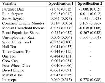
odometer reading and those that don’t. As shown in Table 3.6, these differences are modest. When the sample is broken into three subsamples based on length of vehicle ownership, vehicle char-acteristics and demographic charchar-acteristics are similar across the three subsamples. It should be noted that heavy-duty trucks, and particularly diesel powered heavy-duty trucks, are somewhat less likely to carry an odometer reading than other trucks. By far the strongest determinant of whether an odometer reading is recorded is the vehicle’s initial purchase date, which can be seen in Table 3.7, where I present the results of a logistic regression of an odometer reading dummy variable on a variety of demographic characteristics. This relationship motivates a selection adjustment I use in§5.2.4 to account for non-random entry of odometer readings when estimating my structural model.
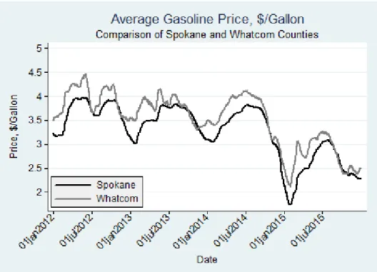
3.2 Fuel Prices
Daily, retailer-level fuel prices are provided by OPIS, who use a variety of means to gather data at the retailer-level on fuel prices in the United States, including fleet cards carried by motor carriers, data scraping, and agreements with individual retailers wherein the retailer will update OPIS with their prices on a frequent basis. As a result of their sampling methodology the quantity of retailers which report a price varies across the sample, but reporting rates are reasonably high and improve throughout the course of the sample. I observe an average of 1,968 retailers in a given day reporting a gasoline price. The count of retailers reporting a gasoline price ranges from a minimum of 1,225 to a maximum of 2,184 throughout the sample. Diesel prices are not reported as frequently, but coverage is still sufficient for the purposes of this project. I observe an average of 1,021 retailers reporting a diesel price on a given day, with the observation count ranging from 384 retailers to 1,298 retailers. It should be noted that the proportion of retailers which sell diesel is significantly higher than the ratio of daily gasoline retailers reporting a price to daily diesel retailers reporting a price, and it appears that the vast majority of retailers in the state sell both gasoline and diesel (see §A.3 for more details).8 The breadth of this data allows me to observe daily fuel prices across the entire state of Washington, which allows me to exploit significant cross-sectional
variation in fuel prices, in addition to time-series variation which is typically seen in a panel of this length. For this project’s purposes, I aggregate fuel prices up to the level of daily county averages for both gasoline and diesel. The aggregation process, and my handling of missing data throughout the course of my sample in certain low population counties, is also described further in§A.3 for the interested reader.
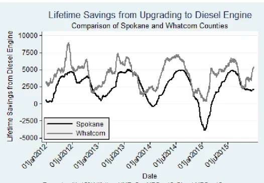
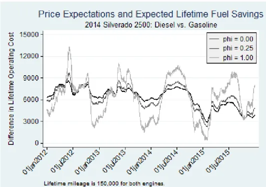
engine which achieves 12 miles per gallon versus a diesel upgrade which achieves 15 miles per gal-lon.9 Figure 3.6 presents the operating cost savings associated with upgrading to the diesel engine and driving 150,000 miles at each county’s fuel price over the course of the vehicle’s life, were the current prices to persist. Depending on the an individual’s location and the date of purchase, operating cost savings associated with adopting the diesel engine range between $0 and $8,000. Comparing different regions of the state, an individual living in Whatcom county typically stands to save between $1,500 and $2,500 more by upgrading to the diesel engine than an individual in Spokane county.
Second, within each county, the diesel premium (as well as the savings associated with upgrad-ing to the diesel engine) exhibits mean-reversion to the county’s average diesel premium. Gaso-line and diesel prices are highly correlated over time as the primary determinant of each fuel’s price is the price of crude oil. However, the diesel premium fluctuates throughout the year due to factors such as seasonality in diesel and gasoline demand, short-term refinery outages, and a variety of other minor factors. Given the durable nature of automobiles, it stands to reason that a forward-looking individual ought to be relatively irresponsive to time-series variation in the diesel premium. For example, consider a consumer who is deciding between the gasoline and diesel variant of a particular truck in Spokane County during July 2015. At this time, the diesel premium was roughly $0.00. If this consumer is aware of the history of the diesel premium, her expectation of the diesel premium over the life of the vehicle should not be $0.00, as it should account for the fact that the average premium in Spokane County has been around $0.50 per gallon. Simply put, forward-looking individuals ought to respond differently to such fuel price variation than they do to more persistent sources of fuel price variation. In §4 and §5 I illustrate the importance of allowing consumers to exhibit a different response to different sources of price variation. For the interested reader, I document the stationarity of the diesel premium for a significantly longer panel of fuel prices in§A.5.10
9These fuel economy figures are similar to those of the gasoline and diesel variants of the Chevrolet Silverado
2500.
3.3 Comparison of User-Generated Fuel Economy Data to EPA Measures
Researchers studying the automobile market in the United States typical use the Environmen-tal Protection Agency’s (EPA) fuel economy ratings as a measure of fuel consumption.11 For each vehicle measured, the EPA releases a separate estimate for city and highway driving, and reports a combined fuel economy measure which is computed as a weighted harmonic mean using 55% city driving and 45% highway driving. These estimates are meant to inform consumers of the fuel efficiency of vehicles being considered for purchase, and in recent years manufacturers have been required by the EPA to post window stickers containing this information on new vehicles. Over the past few decades, a variety of adjustments have been made in methodology for measuring fuel economy with hopes of providing consumers with estimates that are predictive of the vehicles’ fuel consumption. For example, beginning with MY2008, the EPA adjusted their methodology to better account for real-world acceleration, air conditioning usage, and climate conditions. De-spite these changes, researchers have documented significant differences between the EPA’s fuel economy measures and those recorded by individuals operating the vehicles (‘Self-Reported Fuel Economy’). Greene and Lin (2011) consider the relationship between the EPA measures and self-reported measures which were recorded by individuals on the EPA’s “My MPG” system. On this platform, users can record their fuel expenditures and compute their fuel economy, along with recording a variety of individual-level characteristics. When comparing self-reported fuel econ-omy to those which use the EPA’s 2008 methodology, they note that “...the 2008 estimates under-estimate the on-road fuel economy by 14%-16% depending on efficiency level” (Greene and Lin, p. 89).
At the time of this project, the EPA did not produce fuel economy ratings for pickup trucks with a gross vehicle weight rating over 8,500 pounds. As mentioned earlier in this section, roughly one quarter of all new trucks purchased in my sample are heavy-duty trucks which lie above the 8,500 pound threshold and as such, are not rated by the EPA. In order to measure the fuel economy
broader geographic areas to illustrate the mean-reverting nature of the diesel premium.
11As mentioned in the previous section, Leard et al. (2015) use self-reported fuel economy data when considering
of these vehicles, I employ self-reported fuel economy data from fuelly.com, an online platform where individuals can track vehicles’ fuel economy. The platform is well populated, and most truck models in my sample have hundreds of vehicles being tracked by consumers. While the EPA’s “My MPG” system is still on-line, I chose to use fuelly for two important reasons. First, fuelly has a significantly higher number of pickup trucks being tracked. For example, as of 04/22/2017, a total of 114 MY2016 Ford F-150s equipped with the V8 engine option were being tracked on fuelly, whereas only one such vehicle was being tracked on the “My MPG” platform. Second, the “My EPA” system does not allow drivers to track vehicles which are not tested by the EPA, whereas fuelly allows drivers to track a wide variety of vehicles. This allows me to construct measures of fuel economy for heavy-duty pickup trucks.
For a total of seventy-four unique combinations of make-model-series-generation-engine within my sample from the previous section, I extracted self-reported fuel economy data from fuelly.com during June, 2016. For each make-model-series-model year-engine combination, I recorded the number of vehicles being tracked, the total quantity of miles driven, and the average fuel economy, each of which can be easily scraped from fuelly’s interface (for an example, see Figure 3.8).12
I then aggregated this information up from the level of model year to the level of generation in order to increase the sample size of vehicles being tracked.13 Due to the lack of large samples of certain trucks equipped with 2WD, I aggregate fuel economy ratings at the level of make-model-series-generation-engine. Rather than disaggregating down the the level of drivetrain to adjust fuel economy for 4WD trucks, I use differences in EPA ratings for 2WD versus 4WD trucks to adjust vehicles’ fuel economy accordingly (see§A.3 for details).
Abstracting from differences between ‘real-world’ driving styles and the EPA’s attempts to approximate ‘real-world’ driving styles in their fuel economy measures, one might imagine two
12During MY 2015 and MY 2016, the Ford F-150 was offered with two different 3.5 Liter V6 engines, an
entry-level 282 horsepower engine and an upgraded ‘EcoBoost’ engine which is rated at 365 horsepower. Because fuelly users typically only enter engines at the level of displacement and cylinder configuration, I am unable to separate self-reported fuel economy for these two engines in either the 2015 or 2016 model year. In my next chapter, I use the EPA measurements for these configurations.
13Generation is a well-defined concept in the automobile industry. Roughly speaking, each ‘generation’ corresponds
primary reasons self-reported fuel economy could differ from estimates produced by the EPA. First, selection into tracking fuel expenditures and fuel economy is presumably not random. For example, those individuals who are more interested in tracking their fuel economy may also be more likely to drive in a manner which increases fuel efficiency.14 Such a selection mechanism could possibly explain the findings of Greene and Lin (2011), who report that individuals on the “My MPG” platform tend to outperform EPA estimates. Second, the nature of ‘real-world’ driving conditions can be more challenging to define with pickup trucks than other vehicles. Pickup trucks can be used for a wide variety of pleasure and work-related tasks, and fuel economy can decrease significantly when a truck is used to haul a significant amount of payload or tow a heavy trailer. In particular, we might expect that if the propensity to haul payload or tow is higher for larger pickup trucks than smaller pickup trucks, the self-reported measures might be significantly lower for large pickup trucks than the EPA measures.
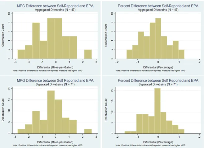
A descriptive analysis of my self-reported measures of fuel economy (SRP) suggest that de-spite the aforementioned concerns, the two different sets of fuel economy measures are strongly correlated. In Figure 3.9, I present a histogram of the differentials between the EPA estimates and the SRP estimates pulled from fuelly. Whether the differentials are computed prior to adjusting for drivetrain differences or after adjusting for differences in drivetrain, the differences are modest. The vast majority of observations lie within ten percent of their corresponding EPA estimates, with no difference more than three miles per gallon. As an additional exercise, I run an OLS regression of the EPA’s fuel economy measurements on my SRP measures:
SRPj =β0+β1EP Aj+j
]
SRPj =β0+β1EP Aj +j
whereSRPjrefers to my fuel economy measurement which is not adjusted for different drivetrains
14Fuel economy gains from ‘hypermiling’ techniques such as coasting into turns, slowly accelerating, and driving
andSRP]j refers to my fuel economy measure which adjusts for different drivetrains. I run each
regression for five different sets of observations based on the quantity of vehicles I observed (Nj)
and the quantity of miles which were recorded by the vehicles (V M Tj), and present the results
in Table 3.8. My measure which adjusts for drivetrain exhibits a mildly higher correlation with the EPA measures, although both measures have a reasonably strong fit, as estimates usingSRPj
result in anR2between 0.750 and 0.788, and estimates usingSRP]
j result in anR2 between 0.787
and 0.820. Unlike Greene and Lin (2011), my regression coefficients do not show evidence of a systemic difference between the EPA’s measures and my SRP estimates. In the five specifications using SRPj the coefficient on the EPA measure ranges between 0.911 and 0.946 whereas the
estimated intercept lies between 0.573 and 1.260. Results are similar when theSRP]j measure is
used, with the coefficient on the EPA measure ranging between 0.951 and 0.975 and the intercept ranging from 0.088 to 0.602. In all ten specifications, ninety-five percent confidence intervals for the coefficients contain both β0 = 0 and β1 = 1. Thus, the systemic difference between SRP
and EPA measures reported in Greene and Lin (2011) does not show up here, possibly allaying concerns about the correlation between drivers’ likelihood of tracking their fuel economy and the extent to which they engage in fuel efficient driving practices.
Table 3.1: Market Shares (%), by Owner Type
All Personal Business Leased Exempt Owner
Observations 124,310 88,667 22,301 9,236 4,106
Avalanche 0.37 0.43 0.28 0.12 0.02
Canyon 0.28 0.29 0.33 0.18 0.00
Colorado 1.57 1.17 1.88 2.65 6.26
Dakota 0.02 0.01 0.06 0.00 0.00
Escalade EXT 0.05 0.05 0.08 0.05 0.00
F-150 19.50 17.64 22.64 26.72 26.35
F-150 SVT 0.64 0.72 0.65 0.12 0.02
F-250 3.87 2.34 6.41 4.60 21.53
F-350 5.09 4.70 6.35 1.78 14.15
Frontier 3.04 2.88 3.52 3.81 1.92
Ram 1500 11.16 11.76 10.21 8.02 10.42
Ram 2500 4.56 5.25 4.07 0.89 0.63
Ram 3500 2.84 3.46 1.99 0.09 0.19
Ranger 0.25 0.24 0.29 0.31 0.05
Ridgeline 0.79 0.98 0.18 0.80 0.00
Sierra 1500 3.18 3.24 3.66 2.79 0.24
Sierra 2500 1.58 1.64 2.13 0.35 0.07
Sierra 3500 0.50 0.56 0.58 0.04 0.00
Silverado 1500 12.64 12.07 15.44 12.57 10.08
Silverado 2500 4.48 3.92 6.93 3.76 4.90
Silverado 3500 2.13 1.94 3.58 0.64 1.88
Tacoma 13.09 15.43 4.88 15.73 1.17
Titan 0.53 0.60 0.52 0.19 0.10
Table 3.2: Selected Descriptive Statistics: All Registration Types
All Trucks Mid Size Full Size Heavy Duty
Observations 124,310 24,165 68,979 31,116
MSRP $37,226 $27,079 $36,728 $46,197
Regular Cab 0.07 0.05 0.06 0.09
Extended Cab 0.26 0.31 0.30 0.14
Crew Cab 0.67 0.64 0.64 0.77
Four Wheel Drive 0.90 0.81 0.92 0.93
Dual Rear Wheels 0.01 0.00 0.00 0.06
Work Truck Trim 0.13 0.12 0.13 0.14
Length (Feet) 22.69 20.76 22.83 23.86
Width (Feet) 7.88 7.40 7.97 8.04
Height (Feet) 7.52 6.98 7.57 7.85
Diesel Engine 0.19 0.00 0.02 0.72
Gas: Torque (100/lb-ft) 349.30 250.19 378.79 393.84
Diesel: Torque (100/lb-ft) 783.30 NA 420.00 801.48
Gas: Horsepower/100 326.96 230.71 355.07 374.16
Diesel: Horsepower/100 381.65 NA 240 388.74
Gas: Miles/Gallon 16.20 18.49 15.91 12.11
Diesel: Miles/Gallon 14.55 NA 22.57 14.15
Table 3.3: Selected Descriptive Statistics: Personal Registrations
All Trucks Mid Size Full Size Heavy Duty
Observations 88,623 19,041 48,508 21,118
MSRP $37,624 $27,388 $37,111 $48,033
Regular Cab 0.03 0.03 0.04 0.01
Extended Cab 0.23 0.30 0.27 0.09
Crew Cab 0.74 0.67 0.69 0.90
Four Wheel Drive 0.94 0.85 0.96 0.99
Dual Rear Wheels 0.01 0.00 0.00 0.05
Work Truck Trim 0.10 0.10 0.11 0.09
Length (Feet) 22.70 20.79 22.89 24.00
Width (Feet) 7.86 7.42 7.97 8.01
Height (Feet) 7.52 6.99 7.57 7.86
Diesel Engine 0.21 0.00 0.02 0.85
Gas: Torque (100/lb-ft) 348.50 253.58 383.55 391.53
Diesel: Torque (100/lb-ft) 782.88 NA 420 801.73
Gas: Horsepower/100 325.18 233.08 358.86 372.01
Diesel: Horsepower/100 379.85 NA 240 387.12
Gas: Miles/Gallon 16.31 18.32 15.78 12.15
Table 3.4: Selected Characteristics of Pickup Truck Models
Model Make Class Model Years $MSRP Diesel Uptake Gas MPG Diesel MPG Crew Cab 4WD Footprint (sqft)
Avalanche Chevrolet SUT 2011-2013 $48,576 14.31 1.00 1.00 175.05
Canyon GMC Midsize 2011-2012, 2014-2016 $33,769 19.39 0.89 1.00 154.24
Colorado Chevrolet Midsize 2011-2012, 2014-2016 $27,940 19.87 0.52 0.65 150.84
Dakota Dodge Midsize 2011 $27,360 16.18 0.00 1.00 156.66
Escalade EXT Cadillac SUT 2011-2013 $69,640 14.20 1.00 1.00 175.60
F-150 Ford 12-Ton 2011-2016 $37,913 16.28 0.62 0.89 183.05
F-150 SVT Ford 12-Ton 2011-2014 $46,161 13.18 0.91 1.00 199.36
F-250 Ford 34-Ton 2011-2016 $43,080 0.43 12.47 14.50 0.48 0.84 189.27
F-350 Ford 1-Ton 2011-2016 $48,278 0.81 11.32 13.26 0.79 0.92 198.06
Frontier Nissan Midsize 2011-2016 $24,752 18.12 0.62 0.78 150.35
Ram 1500 RAM 12-Ton 2011-2016 $35,923 0.17 15.69 22.57 0.50 0.94 180.98
Ram 2500 RAM 34-Ton 2011-2016 $46,446 0.82 12.98 15.18 0.97 0.99 188.44
Ram 3500 RAM 1-Ton 2011-2016 $49,034 1.00 13.20 1.00 1.00 191.82
Ranger Ford Compact 2011 $22,557 20.22 0.00 0.34 139.45
Ridgeline Honda SUT 2011-2014 $35,004 17.37 1.00 1.00 160.97
Sierra 1500 GMC 12-Ton 2011-2016 $39,972 16.40 0.68 0.95 183.02
Sierra 2500 GMC 34-Ton 2011-2016 $47,374 0.70 12.13 14.90 0.80 0.99 190.79
Sierra 3500 GMC 1-Ton 2011-2016 $51,618 1.00 14.01 1.00 1.00 192.56
Silverado 1500 Chevrolet 12-Ton 2011-2016 $36,632 16.40 0.52 0.87 179.68
Silverado 2500 Chevrolet 34-Ton 2011-2016 $43,390 0.51 12.11 14.90 0.65 0.94 189.29
Silverado 3500 Chevrolet 1-Ton 2011-2016 $46,310 0.79 10.51 13.80 0.72 0.86 194.66
Tacoma Toyota Midsize 2011-2016 $26,217 18.56 0.63 0.82 154.01
Titan Nissan 12-Ton 2011-2015 $35,554 13.61 0.84 1.00 178.56
Tundra Toyota 12-Ton 2011-2016 $33,087 14.69 1.00 0.99 182.83
Table 3.5: Yearly Vehicle Miles Traveled
Class Fuel Observations µV M T σV M T
Compact Gasoline 1,465 11,966 6,863
Compact Diesel 0 NA NA
Sport Utility Truck Gasoline 145 12,244 6,053
Sport Utility Truck Diesel 0 NA NA
Half Ton Gasoline 4,087 13,068 7,016
Half Ton Diesel 5 13,842 11,517
Three-Quarter Ton Gasoline 214 12,486 7,283
Three-Quarter Ton Diesel 558 14,946 8,434
One Ton Gasoline 23 10,828 9,749
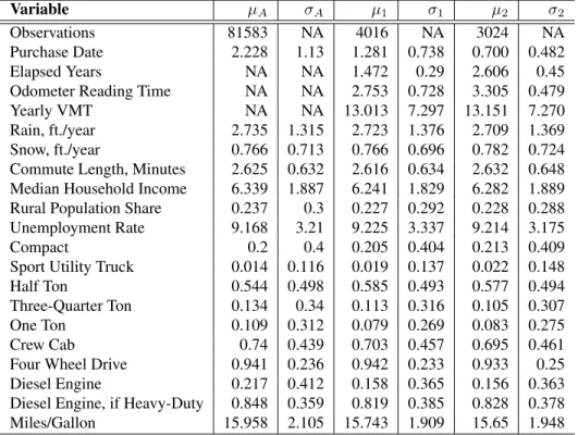
Table 3.6: Summary Statistics, by Length of Ownership
Variable µA σA µ1 σ1 µ2 σ2
Observations 81583 NA 4016 NA 3024 NA
Purchase Date 2.228 1.13 1.281 0.738 0.700 0.482
Elapsed Years NA NA 1.472 0.29 2.606 0.45
Odometer Reading Time NA NA 2.753 0.728 3.305 0.479
Yearly VMT NA NA 13.013 7.297 13.151 7.270
Rain, ft./year 2.735 1.315 2.723 1.376 2.709 1.369
Snow, ft./year 0.766 0.713 0.766 0.696 0.782 0.724
Commute Length, Minutes 2.625 0.632 2.616 0.634 2.632 0.648
Median Household Income 6.339 1.887 6.241 1.829 6.282 1.889
Rural Population Share 0.237 0.3 0.227 0.292 0.228 0.288
Unemployment Rate 9.168 3.21 9.225 3.337 9.214 3.175
Compact 0.2 0.4 0.205 0.404 0.213 0.409
Sport Utility Truck 0.014 0.116 0.019 0.137 0.022 0.148
Half Ton 0.544 0.498 0.585 0.493 0.577 0.494
Three-Quarter Ton 0.134 0.34 0.113 0.316 0.105 0.307
One Ton 0.109 0.312 0.079 0.269 0.083 0.275
Crew Cab 0.74 0.439 0.703 0.457 0.695 0.461
Four Wheel Drive 0.941 0.236 0.942 0.233 0.933 0.25
Diesel Engine 0.217 0.412 0.158 0.365 0.156 0.363
Diesel Engine, if Heavy-Duty 0.848 0.359 0.819 0.385 0.828 0.378
Miles/Gallon 15.958 2.105 15.743 1.909 15.65 1.948
aOwnership A indicates that I do not observe a vehicle transaction which requires an
odometer reading to be taken. Option 1 indicates that between 366 days and 730 days elapsed between a vehicle’s original purchase date and my observed odometer reading. Option 2 indicates that greater than 731 days elapsed between a vehicle’s original purchase date and my observed odometer reading.
bPurchase date gives elapsed time, in years after January 1, 2012, at the time of
ve-hicle purchase. Elapsed years gives number of years the veve-hicle was driven before observing an odometer reading. Odometer Reading Time gives elapsed time, in years after January 1, 2012, at the time of the odometer reading.
cDemographics are specified at the zip-code level, while weather data are specified at
Table 3.7: Logit: Odometer Reading Dummy
Variable Specification 1 Specification 2
Purchase Date -1.076 (0.015) -1.086 (0.015)
Rain, ft./year -0.015 (0.012) -0.011 (0.012)
Snow, ft./year 0.031 (0.023) 0.031 (0.023)
Commute Length, Minutes 0.114 (0.026) 0.109 (0.026) Median Household Income -0.037 (0.008) -0.038 (0.008) Rural Population Share -0.232 (0.052) -0.267 (0.052)
Unemployment Rate 0.006 (0.004) 0.006 (0.004)
Sport Utility Truck -0.233 (0.100)
-Half Ton -0.041 (0.053)
-Three-Quarter Ton -0.244 (0.115)
-One Ton -0.484 (0.151)
-Crew Cab -0.007 (0.031)
-Four Wheel Drive -0.040 (0.066)
-Diesel Engine -0.061 (0.091)
-Miles/Gallon -0.045 (0.015)
-Intercept 0.069 (0.315) -0.770 (0.088)
Table 3.8: OLS Regressions of EPA Combined Fuel Economy on Self-Reported Measures
Measure Sample Observations Slope (β1) Intercept (β0) R2
SRP Nj>0 47 0.911 (0.064) 1.26 (1.038) 0.782
SRP Nj>10 46 0.919 (0.064) 1.097 (1.035) 0.788
SRP Nj>20 40 0.946 (0.082) 0.573 (1.350) 0.750
SRP V M Tj>100K 45 0.922 (0.068) 1.059 (1.096) 0.780 SRP V M Tj>250K 38 0.938 (0.081) 0.759 (1.328) 0.750
]
SRP Nj>0 71 0.951 (0.052) 0.602 (0.872) 0.816
]
SRP Nj>10 70 0.958 (0.052) 0.459 (0.872) 0.820
]
SRP Nj>20 61 0.975 (0.067) 0.088 (1.132) 0.787
]
SRP V M Tj>100K 68 0.955 (0.055) 0.511 (0.924) 0.812
]
Figure 3.1: Lognormal Fit of Diesel VMT Distribution
Figure 3.3: Topographical Map of Washington with Oil Distribution Network
Figure 3.4: Price Difference between Gasoline and Diesel, 01/01/2012-12/31/2015
Figure 3.6: Diesel Price, 01/01/2012-12/31/2015
Figure 3.8: Screenshot of Fuelly Interface
Figure 3.10: Scatterplot of Self-Reported and EPA Measures (A)
SECTION 4
DESCRIPTIVE ANALYSIS
In this section I present descriptive evidence on the determinants of fuel choice and subsequent usage intensity. This subsection is not intended to present or discuss any causal effects, but merely to illustrate patterns present in my data as a means of motivating my structural model, which is presented in§5.
4.1 Descriptive Evidence: Fuel Choice
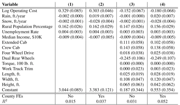
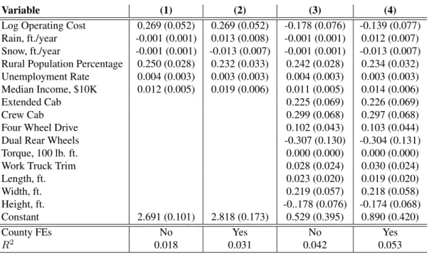
As discussed in the introduction to this paper, the limited adoption of vehicles operating on any fuel other than gasoline has posed challenges for researchers studying fuel choice among U.S. automobile purchasers. The market for pickup trucks has a significantly higher adoption rate of non-gasoline powertrains, as diesel engines have been available in heavy-duty pickup trucks for several decades. In this subsection, I present a descriptive analysis of the determinants of fuel choice among purchasers of heavy-duty trucks. This analysis considers the determinants of fuel choice conditional on purchasing a heavy-duty truck, and as this explicitly ignores substitution between other classes of pickup truck and heavy-duty trucks, the usual caveats apply.1 I estimate a linear-in-parameters binary logit model of the following form:
P r(Diesel|Heavy−Duty) = exp(β0+β1Zi+β2Pi) 1 +exp(β0+β1Zi+β2Pi)
whereZi refers to a vector of local taste-shifters andPi refers to a vector of fuel price data.
Re-sults pertaining to the sample which consists of all registration types (N = 31,166) are presented in Table 4.1, while results pertaining to the sample which consists of only personal registrations (N = 21,118) are presented in Table 4.2. In the appendix, Table B.1 gives results from the sample