Generalized Feistel Schemes
Ivan Tjuawinata, Tao Huang, Hongjun Wu
Division of Mathematical Sciences School of Physical and Mathematical Sciences,
Nanyang Technological University, Singapore [email protected]
[email protected] [email protected]
Abstract. Nachef et al [12] used differential cryptanalysis to study four types of Generalized Feistel Scheme (GFS). They gave the lower bound of maximum number of rounds that is indistinguishable from a random per-mutation. In this paper, we study the security of several types of GFS by exploiting the asymmetric property. We show that better lower bounds can be achieved for the Type-1 GFS, Type-3 GFS and Alternating Feis-tel Scheme. Furthermore, we give the first general results regarding to the lower bound of the Unbalanced Feistel Scheme.
Keywords:Generalized Feistel Network, Differential Analysis, Chosen Ci-phertext Attack, Known Plaintext Attack.
1
Introduction
1.1 Background
1.2 Previous Work
Many analysis on Feistel network and Generalized Feistel Network have been done [7,10,12,14,15,22]. However, as mentioned in [7], most analysis is specialized in some types instead of analysing many types at once.
Nachef et.al. [12] used differential cryptanalysis to study four types of GFS us-ing Known Plaintext Attack (KPA) and Chosen Plaintext Attack (CPA) model. They established lower bounds of the maximum number of rounds distinguish-able in Type-1, Type-2, Type-3 and Alternating Feistel Scheme in the two mod-els.
Provable-security analysis has been applied to Feistel Networks in [10] and [7]. Luby and Rackoff [10] analysed the classical Feistel Networks which is then improved and generalised by Hoang and Rogaway in [7] to analyse Classical, Un-balanced, Alternating, Type-1, Type-2 and Type-3 Generalized Feistel Scheme. The theoretical analysis of Generalized Feistel also plays an important role in design and analysis of practical ciphers. In the design of DEAL [9], Knudsen con-siders this theoretical attack to provide a security bound for any key schedule that is used.
An interesting property existed in many the GFS designs is that the en-cryption and deen-cryption are not exactly the same, which sometimes makes the differential propagation slower in the decryption than in the encryption. In the analysis on Skipjack [4,5], the difference in the decryption has been considered. Recently, Tjuawinata et al. [21] showed that the analysis of Simpira [6] can be improved by considering the asymmetry of Type-1 Generalized Feistel Scheme. While this property is exploited in the cryptanalysis, it is undesired for the de-signer. In the design criterion of Keccak [3], it mentioned the property that the encryption and decryption is symmetric.
1.3 Our Contribution
In this paper, we study the asymmetric property in the Generalized Feistel Schemes. We provide better lower bounds of the maximum number of rounds distinguishable in 3 different types of Generalized Feistel Networks given in [12], which are Type-1 Feistel Scheme, Type-3 Feistel Scheme and Alternating Feistel Scheme.1 We also provide a lower bound of the maximum number of rounds distinguishable in another type of Generalized Feistel Network, the Unbalanced Feistel Network. As far as we know, this is the first result on Unbalanced Feistel Network that is applicable to different values of k0. We exploit the asymmetry
of certain types of GFS by observing that the backward differential diffusion is slower than the forward differential diffusion. This leads to the improvements on the lower bounds.
For Type-1 Feistel Scheme, we provide a chosen ciphertext distinguisher which distinguishesk−1 more rounds than the distinguisher given in [12] with
1 We also examine Type-2 Feistel Scheme, but we cannot improve the previous results
the same complexity. Furthermore, when the number of rounds to distinguish is fixed to ak−2 rounds for some integer a in the range 4 ≤ a ≤ k−1, the distinguisher in this paper has complexity 1/2n of the distinguisher given in the CPA model in [12], from√2·2(a−2)n to√2·2(a−3)n.
In Type-3 Feistel Scheme, [12] only provides lower bound for the case when the number of branches is at least 6.We propose a distinguisher which can be used for any number of branches and can distinguish up tok+ 2 rounds in both KPA and CCA model with complexity√2·2(k−1)nand√2·2(k−2)nrespectively.
When k is at least 6, in the CCA model, a distinguisher for one more rounds than the one given in [12] is constructed.
In Alternating Feistel Scheme, our analysis shows that lower complexity can be achieved in some special cases. More specifically, when the number of round is odd, the complexity is improved by a factor of 232n from the distinguisher
proposed in [12].
In our analysis of Unbalanced Feistel Scheme, letk be the total number of sub-blocks andk0be the number of sub-blocks that are used as the output of the round function. In this paper, we consider two special cases when k0 or k−k0 divides k. When k0 = 1, we can distinguish up to (k2 +k−1) rounds with complexity less than 2kn under KPA model. In the CCA model, the number of rounds that can be distinguished is up to 2krounds with complexity less than 2n. When k0 ≥ 1, a lower bound of the maximum number of rounds that is
distinguishable from random permutation is given. In KPA model, the bound is
k2 k0 −
k
2+
k
k0 whenk0 is even and
k2 k0 −
k(k−1)
2k0 whenk0 is odd. In CCA model, the bound is k2+ 2kk0 whenk0 is even and
k(k0+3)
2k0 whenk0is odd. To the best of our knowledge, this is the first analysis on Unbalanced Feistel Scheme for any values ofk.
1.4 Organization
We give some preliminaries in Section2. The attack overview is then discussed in Section3. The analysis on Type-1 Feistel Scheme is presented in Section4. Sections5and6contains analysis of Type-3 and Alternating Feistel Scheme. The Unbalanced Feistel Scheme is analysed in Section 7. In Section8, we conclude this paper.
2
Preliminaries
2.1 Generalized Feistel Schemes
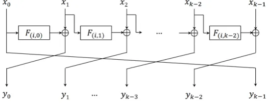
Type-1 Feistel Schemes. Π is an r-round Type-1 Feistel scheme if Π consists ofrrepetitions of µ1 : (F2n)k →(F2n)k where µ1(x0,· · · , xk−1) = (x1⊕Fi(x0), x2,· · · , xk−1, x0). Assume that Fi : F2n → F2n is a function fromn-bit ton-bit which may vary depending on the round where it is being called. Here i = 1,· · ·, r. Illustration of round i of Type-1 Feistel Scheme can be found in Figure1.
Fig. 1.Roundiof Type-1 Feistel Scheme
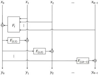
Type-3 Feistel Schemes. Π is an r-round Type-3 Feistel scheme if Π consists ofriterations ofµ3:Fk2n→Fk2n.Given (x0,· · · , xk−1), µ3 maps
(x0,· · ·, xk−1)
to
(x1⊕F(i,0)(x0), x2⊕F(i,1)(x1),· · · , xk−1⊕F(i,k−2)(xk−2), x0).
Illustration of roundiof Type-3 Feistel Scheme can be found in Figure2.
Alternating Feistel Schemes. For this scheme, consider two different round functions µA,0, µA,1 : Fk2n → Fk2n which are used alternatingly for each round.
- µA,0(x0,· · ·, xk−1) = (x0⊕Fi(x1,· · · , xk−1), x1,· · ·, xk−1) where Fi:Fk2−n1→F2n is called in round 2i−1. µA,0 is called the contracting round.
- µA,1(x0,· · ·, xk−1) = (x0, x1⊕F(i,1)(x0),· · ·, xk−1⊕F(i,k−1)(x0)).Here Fi,j :F2n →F2n is the function called in thej-th component in round 2i. These rounds are called the expanding rounds.
Illustration of round 2i−1 and 2iof Alternating Feistel Scheme can be found in Figure3. Note that round number and indexistarts from 1 instead of 0.
Fig. 3.Round 2i−1 and Round 2iof Alternating Feistel Scheme
Alternatively,µA,1 can be used in odd rounds andµA,0 in even rounds but in this paper a contracting round is always used at round 1. Note that if µA,1is used in the first one instead, the backward analysis on this variant is equivalent to the forward analysis discussed in [12].
Unbalanced Feistel Schemes.This is a special case of the UFN defined in Figure 1 of [7]. Letk0 = 1,· · ·, k−1 andF
s:Fk−k
0 2n →Fk
0
2nbe a map from (k−k0)nbit tok0nbit with component functions denoted asFs,0,· · · , Fs,k0−1 with the round numbersas its parameter. ThenΠ is anr-round UFN(k0, k) if it contains r repetitions of µU : Fk2n → Fk2n. In round s, given an input (x0,· · · , xk−1), µU maps it to
(xk0,· · ·, xk−1, x0⊕Fs,0(xk0,· · ·, xk−1),· · ·, xk0−1⊕Fs,k0−1(xk0,· · ·, xk−1)). Illustration of roundsof UFN(k0, k) is given in Figure4.
Fig. 4.Roundsof Unbalanced Feistel Scheme
2.2 Random Variable
Given a random variable X, denote by E(X), V(X), σ(X) the expected value, variance and standard deviation ofX respectively. Note thatV(X) =E(X2)− E(X)2 andσ(X) =p
V(x).
Now givenn random variablesX1,· · ·, Xn, define the covariance ofXi and
Xj asCov(Xi, Xj) =E(XiXj)−E(Xi)E(Xj).A simple calculation of the
def-inition yieldsV(Pn
i=1Xi) = Pn
i=1V(Xi) + P
i6=j,1≤i,j≤nCov(Xi, Xj).
Proposition 1. [12] Let X and Y be two random variables. X is said to be distinguishable from Y if|E(X)−E(Y)| ≥max(σ(X), σ(Y)).
More specifically, letEX, EY be the expected values of X andY respectively
whileσX, σY being the standard deviations ofX andY respectively. Without loss
of generality, letEX< EY. Then, ifEY −EX ≥max(σ(X), σ(Y)),:
1. P r X≥ EX+EY 2
≤0.30854 2. P r Y ≤EX+EY
2
≤0.30854.
Proof. We only prove the first claim since the second one can be proved by using the same method. A simple calculation tells us that:
P r
X ≥EX+EY
2
=P r
X−EX ≥
EY −EX
2
≤P rX−EX ≥
σX
2
=P r
X−E
X
σX
≥ 1
2
By Central Limit Theorem X−EX
Remark 1. When we use this Proposition later, the random variables are actu-ally the number of plaintext-ciphertext pairs that satisfy some equations. Now since the number of plaintext-ciphertext pairs is in the magnitude of 2αn for some constant α,we can apply Central Limit Theorem here. So if the random variable is X with meanµ and standard deviationδ,we can approximate X −δµ by standard normal distribution.
3
Attack Overview
In this paper, as we have discussed in Subsection1.2, we exploit the asymmetry of the scheme by considering the backward differential diffusion.
We will discuss two types of improvements:
Unconstrained environment. We aim for a better lower bound for the maximum number of rounds distinguishable than the bound given in [12]. By unconstrained environment, we mean that analysis considered in this environment aims to distinguish more rounds than the previous results with complexity strictly less than 2knwherekis the number of sub-blocks andnis the number of bit in each sub-blocks. Throughout this paper, the complexity of the attack is measured by the number of query performed to make the attack possible.
Constrained environment.There are two possible forms of this improve-ment. Firstly, we aim to improve number of rounds that can be distinguished in the backward direction given the same complexity as the distinguisher given in [12]. Secondly, given the same number of rounds, we aim to reduce the complexity to distinguish the GFS from a random permutation. Our analysis uses m plaintext-ciphertext pairs and considers the expected number of pairs N that satisfies certain conditions depending on the scheme analysed. LetNpermbe the value ofN for a random permutation andNF be the
valueN forF,ther-round Generalized Feistel Scheme. We use this information to calculate the maximum number of roundsrsuch thatNpermis distinguishable fromNF.
The functionFi (or F(i,j)) used in the round function of GFS is assumed to be ideal keyed functions. Given the input, the output is a random n-bit string. Similarly, since it is ideal, given a nonzero input difference, the output difference is uniformly distributed.
Furthermore, letI1 and I2 be two distinct indices of the round function in the same cryptosystem (Ij can be a single integer or a pair or integers depending
on the GFN we are considering). Given two different indices values I1 and I2, we also assume thatFI1 andF(I2)are independent from each other. Hence given
the same input (or output) difference∆SofFI1 andFI2,we can further assume
that FI2(∆S) is uniformly distributed even assuming thatFI1(∆S) is already
known.
in each stage as∆I−∆1− · · · −∆r−1−∆O.The first step of the attack is done
by expressing ∆I as a function of ∆1,· · · , ∆r−1 and ∆O. We are choosing the
express ∆I as a function of∆O instead of the other way around since we want
to use the expression we get to launch a backward differential trail instead of the forward trail. To enable this, for each ∆, we partition∆ to k sub-blocks. Since each round function takes one of these sub-blocks as input, we can easily find the expression that we need.
Having these expressions, we can then choose carefully the input and output difference (truncated differences) to maximize the probability for the specified input difference focusing in some of the sub-blocks to lead to the output difference chosen. To calculate the success probability, we consider the number of ciphertext pairs with specified difference that can lead to the plaintext pairs with the chosen input difference in two scenarios; when the function is a random permutation, denoted byNpermand when the function is in the form of the Generalized Feistel Network considered, denoted by NF.
Now having the expected values and variances of bothNperm andNF,those
four values will be functions of the round number r and number of ciphertext pairs with the chosen differencem. By Definition1,NF is distinguishable from Nperm if|E(NF)−E(Nperm)| ≥max(σ(NF), σ(Nperm)). So using this inequal-ity, we obtain a relation between the number of rounds r and the number of ciphertext pairsm.This will give us a lower bound of mgivenr. Since we want the distinguisher to be useful, we requiremto be less than the total number of possible ciphertext pairs. In the case of known ciphertext attack, this means that we needm≤2kn.This gives us an upper bound of round numberrsuch thatF
is distinguishable from a random permutation using this backward differential attack.
As we described above, in fact the main idea of the attack is exactly the same for all the types of Generalized Feistel Scheme. We first calculate a re-lation between ciphertext and plaintext differences which is closely related to the structure of the scheme. Once the relation is established, the calculation of the expectation and standard deviation will be very similar and they will be independent of the scheme. Because of this similarity, we will just describe the calculation once and omit the others. In the following sections of this paper, we perform this attack on different types of Generalized Feistel Networks discussed in Subsection2.1.
4
Type-1 Feistel Scheme
4.1 Analysis of the Type-1 Feistel Scheme
Π. In this section we discuss in detail how we build the relations between the sub-blocks, then we discuss how we choose the differential trail. Having the differential trail, the expected value and the variance of the trail when Π is random permutation and a type-1 Generalized Feistel Scheme are calculated. This in turns tells us the maximum number of rounds that is distinguishable from the random permutation using the chosen differential.
LetXi be the intermediate variables obtained in the second branch (indexed
as 1) after thei-th round in the backward direction. By definition of the round function of Type-1 Feistel Scheme, we have the following relations:
X0=Sk−1,
X1=S0⊕Fak+b(Sk−1),
Fort= 2,· · ·, k−1, Xt=Sk+1−t⊕Fak+b−(t−1)(Sk−t),
Fort≥k, Xt=Xt−k⊕Fak+b−(t−1)(Xt−(k−1)),Note that Fr is always used
with inputXak+b−r−k+2.
For r ≥ k−1, the input of the r-th round in the backward direction is (Xr−(k−1), Xr, Xr−1,· · · , Xr−(k−2)).
After r = ak +b rounds, the state becomes (I0,· · ·, Ik−1) where I0 = X(ak+b)−(k−1) and fori= 1,· · ·, k−1, Ii=X(ak+b)−(i−1). The following equal-ities can then be derived using the relations established above:
I0=Xb+1⊕L
a−2
i=0 F(a−i−1)k(Xik+b+2), Forj ∈ {1,· · · ,min(k−1, b+ 1)},
Ij=Xb+1−j⊕ a−1 M
i=0
F(a−i−1)k+j(Xik+(b+2−j)),
Forj ∈ {min(k−1, b+ 1) + 1,· · ·, k−1},
Ij=Xk+b+1−j⊕ a−2 M
i=0
F(a−i−2)k+j(Xik+(k+b+2−j)).
In particular, forI1,
I1=Xb⊕ a−1 M
i=0
F(a−i−1)k+1(Xik+(b+1))
=Xb⊕ a−2 M
i=0
F(a−i−1)k+1(Xik+(b+1))⊕F1(I0)
=
S1⊕La−2
i=0F(a−i−1)k+1(Xik+1)⊕F1(I0) if b= 0 S0⊕Fak+1(Sk−1)⊕L
a−2
i=0F(a−i−1)k+1(Xik+2)⊕F1(I0) if b= 1 Sk+1−b⊕Fak+1(Sk−b)⊕L
a−2
i=0 F(a−i−1)k+1(Xik+(b+1))
We can further expand the sum by noting that wheni= 0,the summand is F(a−i−1)k+1(Xb+1) and
Xb+1=
S0⊕Fak(Sk−1) if b= 0 Sk−b⊕Fak(Sk−b−1) if 1≤b≤k−2 S1⊕Fak(S0⊕Fak+(k−1)(Sk−1)) if b=k−1.
So in any value of b ∈ {0,· · ·, k −1,}, we can express I1 as a function of several sub-blocks of the output Sj, F1(I0) and a−2 terms determined by
intermediate variables. More specifically, forb∈ {0,· · · , k−1},we have:
1. Whenb= 0,
I1⊕S1⊕F1(I0) =
a−2 M
i=1
F(a−i−1)k+1(Xik+1)⊕F(a−1)k+1(S0⊕Fak(Sk−1)), (1)
2. Whenb= 1,
I1⊕S0⊕F1(I0) =
a−2 M
i=1
F(a−i−1)k+1(Xik+2)⊕F(a−1)k+1(Sk−1⊕Fak(Sk−2)), (2)
3. When 2≤b≤k−2,
I1⊕Sk+1−b⊕F1(I0) =
a−2 M
i=1
F(a−i−1)k+1(Xik+2)⊕F(a−1)k+1(Sk−b⊕Fak(Sk−b−1)), (3)
4. Whenb=k−1,
I1⊕S2⊕F1(I0) =
a−2 M
i=1
F(a−i−1)k+1(Xik+1)⊕F(a−1)k+1(S1⊕Fak(S0⊕F(a+1)k−1(Sk−1))).(4)
To choose the truncated differential for each case, we try to utilize Equations 1,2,3and4.We will describe how we choose it for the case whenb= 0.The same idea can then be applied to all the other cases.
Note that for this case, for any ciphertext and its plaintext, we have the relation
I1⊕S1⊕F1(I0) =
a−2 M
i=1
Now for any two ciphertexts C = (S0,· · · , Sk−1), C0 = (S00,· · · , S0k−1) that we choose (and their corresponding plaintextsP = (I0,· · · , Ik−1), P0= (I00,· · · , Ik0−1)), we can only determine the value in the left hand side of Equation1. So based on this relation, we try to find the probability thatI1⊕S1⊕F1(I0) =I10⊕S10⊕F1(I00). Since F1 is always assumed to be ideal, after some rearrangement, this proba-bility is the same as the probaproba-bility that:
1. I0 = I00 2. I1⊕I10 =S1⊕S10.
So we will use this as the truncated differential for the case of Type-1 Scheme with b= 0. As mentioned before, this is done by collectingmciphertexts with their respective plaintexts and we compute the number of ciphertext pairs (along with their corresponding plaintexts) that satisfies the above conditions. The same analysis is done to all the other cases.
Now to find a theoretical approximation for the probability of these con-ditions to be satisfied in various cases, we use the fact that if I0 = I00 and I1⊕I10 =S1⊕S10,we must have
a−2 M
i=1
F(a−i−1)k+1(Xik+1)⊕F(a−1)k+1(S1⊕Fak(S0⊕F(a+1)k−1(Sk−1)))
is equal to
a−2 M
i=1
F(a−i−1)k+1(Xik0 +1)⊕F(a−1)k+1(S01⊕Fak(S00 ⊕F(a+1)k−1(Sk0−1))).
Now note that in this last equation, we have terms that are just functions of S0, Sk−1, S00 and S0k−1. So in the chosen ciphertext attack, to increase the probability, we can make sure that these terms are equal in both sides by making sure thatS0=S00andSk−1=Sk0−1.So in the chosen ciphertext attack, instead of choosing m random ciphertexts, we choose them with their first and last sub-blocks being fixed to a predetermined value.
In summary, out of the m plaintext-ciphertext pairs, we count the number of (s, t),1≤s < t≤msuch that
1. I0(s) = I0(t)
2. I1(s)⊕I1(t) =
S1(s)⊕S1(t) if b= 0 S0(s)⊕S0(t) if b= 1 Sk+1−b(s)⊕Sk+1−b(t) if 2≤b≤k−1.
. (5)
Ifb= 0,pick all the ciphertext with fixed values ofS0(s) andSk−1(s).Hence in the CCA attack,m≤2(k−2)n.
If b = 1,· · · , k−2, fix the values of Sk−b(s) and Sk−b−1(s) for all s = 0,· · ·, m−1.Again, in the CCA attack,m≤2(k−2)n.
Ifb =k−1 and k ≥4, fix the values of S0(s), S1(s) andSk−1(s) for s= 0,· · ·, m−1.In this case, the CCA attack must havemto be at most 2(k−3)n. So in summary, the differential trail for r = ak +b rounds where b ∈ {0,· · ·, k−1}is as follows:
1. In KPA setting, the input (ciphertext) differential is (∇0,· · · ,∇k−1) while the output (plaintext) differential is (∆0,· · ·, ∆k−1) where it satisfies the following equations:
- ∆0= 0.
- ∆1=∇(k+1−b) (modk)
- All other sub-blocks difference is arbitrary, which we denote by?. 2. In CCA setting, the differential is the same, however, we impose some
re-quirement to the ciphertext that we pick:
- Ifb= 0,we fix the value ofS0(s) andSk−1(s).
- Ifb= 1,· · ·k−2,the values of Sk−b(s) andSk−b−1(s) are fixed. - Ifb=k−1,we fix the values of S0(s), S1(s) andSk−1(s).
Let NF,M be the random variable representing the number of sets of two plaintext-ciphertext pairs that satisfy the conditions given by (5) for F rep-resenting the function used, which has value in the set {perm,F }, and M ∈ {KPA,CCA}. F = perm is used for the random permutation while F = F is used for ther-round Type-1 Feistel Scheme.
Now it is easy to see that the probability that the requirement set above to be true is equal to the probability that the right hand side of the equations to agree, which can be computed since we can assume all the Xi is uniformly and
independently distributed by the ideality of the round function (which has been discussed in Section3).
Calculating the expected values and variance of the random variables,
E(N(perm,KPA)), E(N(perm,CCA)), V(N(perm,KPA)), V(N(perm,CCA))
are all approximately 2m·222n.Calculating the random variables corresponding to
F, the expected values and variances are summarised in Table3 which can be found in AppendixA. The details on the calculation of the expected values and variances of NF,CCA forb = 0 can be found in Appendix B. The other results can be calculated using the same method.
Using the proposition of distinguishability of two random variables given in the preliminaries, the result is provided in Table1.
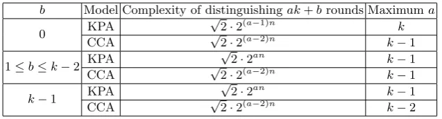
In the KPA model, the maximum number of rounds isk2 where fromk(k−
Table 1: Summary of Distinguishability of Type-1 Feistel Scheme b Model Complexity of distinguishingak+brounds Maximuma
0 KPA
√
2·2(a−1)n k
CCA √2·2(a−2)n k−1
1≤b≤k−2 KPA
√
2·2an k−1
CCA √2·2(a−2)n k−1
k−1 KPA
√
2·2an k−1
CCA √2·2(a−2)n k−2
4.2 Comparison with Existing Result from [12]
To compare with the result given in [12] first note that there are some constants multiplier that are omitted in [12]. More specifically, all the expected values and variances should be multiplied by 12. This constant adjustment comes from the fact that givenmplaintext-ciphertext pairs, the number of sets of 2 distinct pairs should be m(m2−1) ≈m2
2 instead ofm
2.Although the constant multiplier is very close to one compared to 2n,it affects the maximum number of rounds that can
be distinguished in the KPA and CPA model. This is because all the complexities of distinguishers should be multiplied by a factor of √2. The existence of this factor makes it impossible forato reach the maximum number given in [12]. For ak−2 rounds distinguished in KPA model, the complexity should be√2·2(a−2)n.
Hence the maximum number of rounds that can be distinguished in KPA model isk2+k−2 rounds instead ofk2+ 2k−2 rounds. Similarly, forak−1 rounds to be distinguishable in CPA, the complexity is again√2·2(a−2)n.This leads to the maximum number of rounds that is distinguishable in CPA model isk2−1 rounds instead ofk2+k−1.
Note that in both cases, the maximum number of rounds distinguishable without any complexity constraint is still better in the forward direction. So in this section, the advantage of using the backward direction analysis in a constrained environment is discussed.
We compare the results in the CCA model presented above with the CPA model.
1. When the complexity is fixed to √2 ·2tn, in CPA model, the maximum
number of rounds that is distinguishable is (t+ 2)k−1 rounds while in CCA model, the maximum number of rounds that is distinguishable is (t+ 2)k+ (k−2) = (t+ 3)k−2 = (t+ 2)k−1 +k−1rounds which is an increase of k−1 rounds.
2. Suppose that we want to distinguish r rounds for some positive integerr. Table 3 of [12] (after the adjustment by a factor of √2) tells us that when pk−(p−2) = (p−1)k+k−p+ 2≤r≤(p+ 1)k−p=pk+k−p,the complexity is √2·2(p−2)n. Using the same bound for r, the complexity is
√
Now for all the following sections, since the method that is being used is exactly the same, we will not discuss in detail on how to choose the differential, the expected values and the distinguishability. Instead, only the final results will be stated and compared. We note that since we are using Proposition1, which is also used in the analysis in [12], has success probability at least 70 percents.
5
Type-3 Feistel Scheme
5.1 Analysis of the Type-3 Feistel Scheme
As before, we denote the input as S0,· · ·, Sk−1. Define intermediate variables
Xisuch that (Xtk,· · ·, Xtk+k−1) is the state value aftertrounds. Assuming the number of rounds is r, for 0≤s≤k−1, Xs =Ss and Xrk+s =Is. Given the
input of roundc,1≤c≤r, by definition:
Xck=X(c−1)k+k−1
Xck+s=X(c−1)k+(s−1)⊕F(r+1−c,s−1)(Xck+s−1), ∀1≤s≤k−1.
Letr=ak+b for 0≤b≤k−1.In this paper, we only consider a= 1 and b > 0. Expanding the equation for X(k+b)k+s using the equation given above,
the following can then be derived:
• Whenb=s,
X(k+b)k+s= b−1 M
i=0
F(i+1,s−1−i)(X(k+b−i)k+(s−1−i)
⊕ k−2 M
i=0
F(i+b+2,k−2−i)(X(k−1−i)k+(k−2−i))⊕S0.
• Whenb=s+ 1≤k−1,
X(k+b)k+s= s−1 M
i=0
F(i+1,s−1−i)(X(k+b−i)k+(s−1−i))⊕F(b+1,k−2)(X(k)k+k−2)
⊕ k−3 M
i=0
• Whens+ 1< b≤k−1,
X(k+b)k+s= s−1 M
i=0
F(i+1,s−1−i)(X(k+b−i)k+(s−1−i))
⊕ b−s−1
M
i=0
F(s+i+2,k−2−i)(X(k+b−s−1−i)k+k−2−i)
⊕
k−b+s−2 M
i=0
F(i+b+2,k−b+s−2−i)(X(k−1−i)k+k−b+s−2−i)
⊕ b−s−2
M
i=0
F(k+s+i+2,k−2−i)(X(b−s−1−i)k+(k−2−i))⊕Sk−1.
• Whens=b+ 1≤k−1,
X(k+t)k+b = b
M
i=0
F(i+1,b−i)(X(k+b−i)k+b−i)
⊕ k−3 M
i=0
F(i+3,k−2−i)F(X(k−2−i)k+(k−2−i)⊕S1.
• Whenb+ 1< s≤k−1,
X(k+b)k+s= b
M
i=0
F(i+1,b−i)(X(k+b−i)k+b−i)
⊕ s−b−2
M
i=0
F(b+i+2,s−b−2−i)(X(k−1−i)k+s−b−2−i)
⊕
k−s+b−2 M
i=0
F(s+2+i,k−2−i)(X(k−s+b−1−i)k+(k−2−i))⊕Ss−b.
Letb∈ {1,· · ·, k−1}.For themplaintext-ciphertext pairs, the distinguishing attack counts the number of sets of two pairs (j, j0),1≤j < j0≤mthat satisfies the following two conditions:
1. I(r−1)(j) = I(r−1)(j0) 2. Ir(j)⊕Ir(j0) =S0(j)⊕S0(j0).
(6)
In the CCA model, fix the value ofSk−1(j) of all them ciphertexts. Hence m≤2(k−1)n.
Calculating the random variables with the same method, E(N(perm,KPA)), V(N(perm,KPA)), E(N(perm,CCA)), V(N(perm,CCA)), V(N(F,KPA)) and
V(N(F,CCA)) are all approximately m
2
2·22n while
E(N(F,KPA)) = m2
2
1 22n +
1 2(k+r−2)n
and
E(N(F,CCA)) = m2
2 1
22n +
1 2(k+r−3)n
.
In both KPA and CPA model,F is distinguishable from a random permutation when there are up tok+ 2 rounds and the complexity to distinguishk+brounds are√2·2(k+b−3)n and√2·2(k+b−4)n respectively.
5.2 Comparison with Existing Result from [12]
Now we compare our result with the one given in [12]. First of all, note that in [12], there is a restriction thatk
2
≥3. This means that k needs to be at least 6 while the distinguisher proposed above can be used for allk≥2.So in any attack model, this analysis provides a new lower bound of the maximum number of distinguishable round for 2 ≤ k ≤ 5. Furthermore, when k ≥ 6, in KPA model, in bothk+ 1 andk+ 2 rounds proposed above, the complexity is higher than the one given in [12]. The same thing happen in the distinguisher fork+ 1 rounds in CCA model. However, the lower bound of maximum number of rounds distinguishable from random permutation in CCA model is increased tok+ 2 fromk+ 1 proposed in [12].
6
Alternating Feistel Scheme
6.1 Analysis of Alternating Feistel Scheme
We divide this section to two cases based on the parity of the number of rounds. This is required due to the different round function in odd and even rounds.
Even Number of Rounds Suppose that the number of rounds is 2r.Let Xi
be intermediate variables such that after 2t rounds the state value is (Xtk,· · ·Xtk+k−1).
For any 0≤s≤k−1,(Is, Ss) = (Xrk+s, Xs).Then, given the state value after 2t
rounds, (Xtk,· · ·Xtk+k−1) where 0≤t≤r−1,we have the following relations:
• X(t+1)k=Xtk⊕F(r−t)((Xtk+s⊕F(r−t,s)(Xtk))ks=1−1) where
(Ya)sa=r:= (Yr, Yr+1,· · ·Ys). • X(t+1)k+s=Xtk+s⊕F(r−t,s)(Xtk), ∀s= 1,· · ·, k−1.
Then expand the equation forIs: • I0=S0⊕Lr−1
i=0F(r−i)((Xik+s⊕F(r−i,s)(Xik))ks=1−1)
• ∀s∈ {1,· · ·, k−1},
Is=Ss⊕ r−1 M
i=0
F(r−i,s)(Xik) =Ss⊕F(r,s)(S0)⊕
r−1 M
i=1
The distinguishing attack finds the number of sets of two plaintext ciphertext pairs (p, q),1≤p < q≤m such that they satisfy the following conditions:
1. I0(p) = I0(q)
2. ∀s= 1,· · ·k−1, Ib(p)⊕Ib(q) =Sb(p)⊕Sb(q).
(7)
Furthermore, in CCA model, all the ciphertexts are chosen such that they have the same fixed value inS0(p). So we have,m≤2(k−1)n.
Using the same calculation as before,E(N(perm,KPA)), V(N(perm,KPA)), E(N(perm,CCA)), V(N(perm,CCA)), V(N(F,KPA)) andV(N(F,KPA)) can all be ap-proximated by m2
2·2kn.Furthermore,
E(N(F,KPA)) = m2
2
1 2kn +
1 2rn
andE(N(F,CCA)) = m2
2
1 2kn +
1 2(r−1)n
.
Simplifying this, to distinguish 2r rounds, the complexity is √2·2(r−k
2)n for
KPA and √2·2(r−k
2−1)n for CCA. So when k is even, in both models, F can
be distinguished from a random permutation when the round number is up to 3k−2 with complexity√2·2(k−1)nand√2·2(k−2)nrespectively. Whenkis odd, F can be distinguished from a random permutation when the round number is up to 3k−1. In this case, the complexity is √2·2(k−12)n and
√
2·2(k−32)n
respectively.
Odd Number of Rounds Suppose that the number of rounds is 2r+ 1 for some non-negative integersr.LetXi be intermediate variables such that for any
non-negative integert,after 2t+ 1 rounds, the state value is (Xtk,· · ·, Xtk+k−1). SoIs=Xrk+sfor all 0≤s≤k−1 while
Xs=
Ss, ifs= 1,· · ·, k−1,
S0⊕Fr+1(S1,· · ·, Sk−1) ifs= 0.
Following the expansion done before, the following equalities can be found:
• I0=S0⊕Fr+1(S1,· · ·, Sk−1)⊕L
r−1
i=0 F(r−i)((Xik+s⊕F(r−i,s)(Xik))ks=1−1)
• ∀s = 1,· · ·, k −1, Is = Ss ⊕L r−1
i=0 F(r−i,s)(Xik) = Ss⊕F(r,s)(S0)⊕ Lr−1
i=1 F(r−i,s)(Xik).
Because of this, all the distinguisher and calculation considered in the even number of rounds case can still be used in this case. Hence the complexity to distinguish 2r+ 1 rounds is √2·2(r−k2)n for KPA and
√
2·2(r−k2−1)n for
CCA. When kis even, in both models, F can be distinguished from a random permutation when the round number is up to 3k−1 with complexity√2·2(k−1)n and√2·2(k−2)nrespectively. Whenkis odd, we can distinguish up to 3krounds with complexity√2·2(k−12)n and
√
6.2 Comparison with Existing Result from [12]
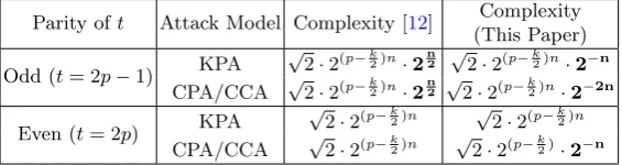
We compare the result of previous subsection with the one given in Section 4.4 in [12]. As before, note all the expected values and variance should be multiplied by 12, all the complexities should be multiplied by √2 and hence maximum number of rounds, in this case, should be decreased by 2.After this adjustment, to distinguisht rounds, the complexities are summarised in Table2:
Table 2: Summary of Comparison of Alternating Feistel Schemes with fixed number of roundst.
Parity oft Attack Model Complexity [12] Complexity (This Paper) Odd (t= 2p−1) KPA
√
2·2(p−k2)n·2
n 2
√
2·2(p−k2)n·2−n
CPA/CCA √2·2(p−k2)n·2n2
√
2·2(p−k2)n·2−2n
Even (t= 2p) KPA
√
2·2(p−k2)n
√
2·2(p−k2)n
CPA/CCA √2·2(p−k
2)n
√
2·2(p−k
2)·2−n
In both models, when the number of rounds is odd, the complexity is better than the forward direction, which is a reduction by a factor of 232n. However,
when the number of rounds is even, backward direction requires the same com-plexity in the KPA model. In the CCA model, the comcom-plexity of backward direction is reduced by a factor of 2n.
Note that after the adjustment to the result in [12], backward differential analysis achieves 2 more rounds in both models, from 3k−2 rounds to 3krounds.
7
Unbalanced Feistel Scheme
7.1 Analysis of Unbalanced Feistel Scheme
In this section we only consider two special cases of UFN(k0, k). We discuss the analysis of the case when k is divisible by k0. This is a generalization of the UFN discussed in Section 6 of [16] where k is set to be 3 and k0 is set to be 1. It can also be seen as a generalization of the UFN discussed in [17] where k0 = 1. In AppendixD, the case whenk−k0 is a factor ofkis considered. Due to the similarity of the technique used and also the page restriction, the detail of the analysis is omitted. This second case is a generalization of the analysis of UFN(k0, k) whenk0=k−1 in [18,8,23].
Analysis of UFN(k0, k) whenk0divides k. LetAbe a positive integer such thatk=Ak0.Define intermediate variablesXisuch that (Xsk,· · ·Xsk+(k−1)) is the state value aftersrounds. So
Suppose that the number of rounds is r = pA+q where 0 ≤ q ≤ A−1. So (Xrk,· · · , Xrk+k−1) = (I0,· · · , Ik−1). Given the state value after s−1(s≥ 1) backward rounds (X(s−1)k,· · ·, X(s−1)k+k−1),the output of the s-th backward round can be computed by:
• Xsk+t=X(s−1)k+(t−k0) ifk0 ≤t≤k−1,
• Xsk+t=X(s−1)k+(k−k0+t)⊕Fr+1−s,t(X(s−1)k,· · ·X(s−1)k+k−k0−1) = X(s−1)k+(k−k0+t)⊕Fr+1−s,t(Xsk+k0,· · ·, Xsk+k−1) if 0≤t≤k0−1. Now for 0≤t≤k0−1,expanding the relation given above, we get:
• Ifq= 0,
It=St⊕ p−1 M
s=1
FsA+2,t(X(r−sA)k+k0,· · ·, X(r−sA)k+k−1)
⊕F2,t(Ik0,· · · , Ik−1),
• Otherwise,
It=S(A−q)k0+t⊕
p
M
s=1
FsA+2,t(X(r−sA)k+k0,· · ·, X(r−sA)k+k−1)
⊕F2,t(Ik0,· · ·, Ik−1).
The distinguisher counts the number of set of two plaintext ciphertext pairs (i, j),1≤i < j≤msuch that
∀t= 0,· · ·, k0−1, It(i)⊕It(j) =S(a−q)k0+t(i)⊕S(a−q)k0+t(j).
In CPA model, pick ciphertexts with a fixed value in Ik0,· · ·, Ik−1. In other words, the maximum number of plaintext-ciphertext pairs ism≤2k0n.
The expected values and variances of the random variables are given in Table 4 in AppendixA
Using the definition of distinguishable, the complexity and maximum number of rounds distinguishable are summarised in Table5and6given in the Appendix C.
A distinguisher for backward direction UFN(k0, k) can be constructed by
considering the forward propagation of the equation. Hence, given the value of Xsk,· · · , Xsk+k−1,we have:
• Xsk+t=X(s+1)k+(t+k0)if 0≤t≤k−k0−1,
• Xsk+t=X(s+1)k+(t−k+k0)⊕Fr−s,t(X(s+1)k+k0,· · ·X(s+1)k+k−1) = X(s+1)k+(t−k+k0)⊕Fr−s,t(Xsk,· · ·, Xsk+k−k0−1) ifk−k0 ≤t≤k−1.
ExpandingSt,the following equalities can be obtained: • Ifq= 0,
St=It⊕ p−1 M
s=1
• Otherwise,
St=It−(A−q)k0⊕
p
M
s=1
Fr−sA,t(XiAk,· · · , XiAk+k−k0−1)
⊕Fr,t(S0,· · ·, Sk−k0−1).
The distinguisher finds the number of sets of two plaintext-ciphertext pairs (i, j) such that∀t=k−k0,· · ·k−1, St(i)⊕St(j) =It−(A−q)k0(i)⊕It−(A−q)k0(j) whereS0,· · ·Sk−k0−1are fixed in the CCA model. It is easy to see that with this model, we have exactly the same expected values, variances and distinguishabil-ity as the ones found in Table4,5and 6.
8
Conclusion
In this paper, differential analysis on the inverse function of four different types of generic Generalized Feistel Scheme, namely Type-1, Type-3, Alternating Scheme and UFN(k0, k) was considered. We show that for Type-1 Feistel Scheme, back-ward distinguisher performs better especially in the chosen ciphertext attack compared to the results in [12]. Using the same complexity, we can distinguish k−1 more rounds while distinguishing the same number of rounds requires smaller complexity with factor of 21n.
In Type-2 and Alternating Feistel scheme, although there are some difference in the complexity, both directions can achieve almost the same number of rounds. This shows that these two types can be seen as almost symmetric from both direction.
We improve the differential cryptanalysis in Type-3 Feistel Scheme in several cases. In KPA model with low number of branches, 2 ≤ k ≤ 5, our analysis provides a lower bound of the number of rounds that is indistinguishable from random permutation. Secondly, in CCA model, the lower bound of maximum number of rounds distinguishable is increased by 1 round, from k+ 1 obtained in [12] tok+ 2.
In Alternating Feistel Scheme, we achieve 2 more rounds than the one claimed in [12]. The complexity is reduced by a factor of 232n when distinguishing the
same odd number of rounds.
Lastly, a lower bound for the maximum number of rounds that is distin-guishable from random permutation in UFN(k0, k) scheme is given through the forward direction distinguisher. To the best of our knowledge, this is the first bound given in a rather general case in which k0 is arbitrary as long as k0 is a divisor ofkfor any integerk.
References
2. Kazumaro Aoki, Tetsuya Ichikawa, Masayuki Kanda, Mitsuru Matsui, Shiho Mo-riai, Junko Nakajima, and Toshio Tokita. Camellia: A 128-Bit Block Cipher Suit-able for Multiple Platforms — Design and Analysis. In Douglas R. Stinson and Stafford Tavares, editors,Selected Areas in Cryptography: 7th Annual International Workshop, SAC 2000 Waterloo, Ontario, Canada, August 14–15, 2000 Proceedings, pages 39–56, Berlin, Heidelberg, 2001. Springer Berlin Heidelberg.
3. Guido Bertoni, Joan Daemen, Micha¨el Peeters, and Gilles Van Assche. Keccak Sponge Function Family Main Document. Submission to NIST (Round 2), 2009. 4. Eli Biham, Alex Biryukov, Orr Dunkelman, Eran Richardson, and Adi Shamir.
Initial Observations on Skipjack: Cryptanalysis of Skipjack-3XOR. In Stafford Tavares and Henk Meijer, editors, Selected Areas in Cryptography: 5th Annual International Workshop, SAC’98 Kingston, Ontario, Canada, August 17–18, 1998 Proceedings, pages 362–375, Berlin, Heidelberg, 1999. Springer Berlin Heidelberg. 5. Eli Biham, Alex Biryukov, and Adi Shamir. Cryptanalysis of Skipjack Reduced
to 31 Rounds Using Impossible Differentials. In Jacques Stern, editor,Advances in Cryptology — EUROCRYPT ’99: International Conference on the Theory and Application of Cryptographic Techniques Prague, Czech Republic, May 2–6, 1999 Proceedings, pages 12–23, Berlin, Heidelberg, 1999. Springer Berlin Heidelberg. 6. Shay Gueron and Nicky Mouha. Simpira v2: A Family of Efficient Permutations
Using the AES Round Function. In Advances in Cryptology–ASIACRYPT 2016: 22nd International Conference on the Theory and Application of Cryptology and Information Security, Hanoi, Vietnam, December 4-8, 2016, Proceedings, Part I 22, pages 95–125. Springer, 2016.
7. Viet Tung Hoang and Phillip Rogaway. On Generalized Feistel Networks. In Tal Rabin, editor,Advances in Cryptology – CRYPTO 2010: 30th Annual Cryptology Conference, Santa Barbara, CA, USA, August 15-19, 2010. Proceedings, pages 613–630, Berlin, Heidelberg, 2010. Springer Berlin Heidelberg.
8. Charanjit S. Jutla. Generalized Birthday Attacks on Unbalanced Feistel Networks. In Hugo Krawczyk, editor,Advances in Cryptology — CRYPTO ’98: 18th Annual International Cryptology Conference Santa Barbara, California, USA August 23– 27, 1998 Proceedings, pages 186–199, Berlin, Heidelberg, 1998. Springer Berlin Heidelberg.
9. Lars Knudsen. DEAL - A 128-bit Block Cipher. InNIST AES Proposal, 1998. 10. Michael Luby and Charles Rackoff. How to Construct Pseudo-random
Permuta-tions from Pseudo-random FuncPermuta-tions. In Hugh C. Williams, editor, Advances in Cryptology — CRYPTO ’85 Proceedings, pages 447–447, Berlin, Heidelberg, 1986. Springer Berlin Heidelberg.
11. Stefan Lucks.Faster Luby-Rackoff ciphers, pages 189–203. Springer Berlin Heidel-berg, Berlin, HeidelHeidel-berg, 1996.
12. Val´erie Nachef, Emmanuel Volte, and Jacques Patarin. Differential Attacks on Generalized Feistel Schemes. In Michel Abdalla, Cristina Nita-Rotaru, and Ri-cardo Dahab, editors, Cryptology and Network Security: 12th International Con-ference, CANS 2013, Paraty, Brazil, November 20-22. 2013. Proceedings, pages 1–19, Cham, 2013. Springer International Publishing.
14. Jacques Patarin. Generic Attacks on Feistel Schemes. In Colin Boyd, editor, Advances in Cryptology — ASIACRYPT 2001: 7th International Conference on the Theory and Application of Cryptology and Information Security Gold Coast, Australia, December 9–13, 2001 Proceedings, pages 222–238, Berlin, Heidelberg, 2001. Springer Berlin Heidelberg.
15. Jacques Patarin. Security of Random Feistel Schemes with 5 or More Rounds. In Advances in Cryptology - CRYPTO 2004, 24th Annual International Cryptology Conference, Santa Barbara, California, USA, August 15-19, 2004, Proceedings, volume 3152 ofLecture Notes in Computer Science, pages 106–122. Springer, 2004. 16. Jacques Patarin. Security of Balanced and Unbalanced Feistel Schemes with Lin-ear Non Equalities. Cryptology ePrint Archive, Report 2010/293, 2010. http: //eprint.iacr.org/2010/293.
17. Jacques Patarin, Val´erie Nachef, and Cˆome Berbain. Generic Attacks on Un-balanced Feistel Schemes with Contracting Functions. In Xuejia Lai and Kefei Chen, editors, Advances in Cryptology – ASIACRYPT 2006: 12th International Conference on the Theory and Application of Cryptology and Information Secu-rity, Shanghai, China, December 3-7, 2006. Proceedings, pages 396–411, Berlin, Heidelberg, 2006. Springer Berlin Heidelberg.
18. Jacques Patarin, Val´erie Nachef, and Cˆome Berbain. Generic Attacks on Un-balanced Feistel Schemes with Expanding Functions. In Kaoru Kurosawa, edi-tor,Advances in Cryptology – ASIACRYPT 2007: 13th International Conference on the Theory and Application of Cryptology and Information Security, Kuching, Malaysia, December 2-6, 2007. Proceedings, pages 325–341, Berlin, Heidelberg, 2007. Springer Berlin Heidelberg.
19. Bruce Schneier and John Kelsey. Unbalanced Feistel networks and block cipher design, pages 121–144. Springer Berlin Heidelberg, Berlin, Heidelberg, 1996. 20. Taizo Shirai, Kyoji Shibutani, Toru Akishita, Shiho Moriai, and Tetsu Iwata. The
128-Bit Blockcipher CLEFIA (Extended Abstract). In Alex Biryukov, editor,Fast Software Encryption: 14th International Workshop, FSE 2007, Luxembourg, Lux-embourg, March 26-28, 2007, Revised Selected Papers, pages 181–195, Berlin, Hei-delberg, 2007. Springer Berlin Heidelberg.
21. Ivan Tjuawinata, Tao Huang, and Hongjun Wu.Cryptanalysis of Simpira v2, pages 384–401. Springer International Publishing, Cham, 2017.
22. Joana Treger and Jacques Patarin. Generic Attacks on Feistel Networks with Internal Permutations. In Bart Preneel, editor, Progress in Cryptology – AFRICACRYPT 2009: Second International Conference on Cryptology in Africa, Gammarth, Tunisia, June 21-25, 2009. Proceedings, pages 41–59, Berlin, Heidel-berg, 2009. Springer Berlin Heidelberg.
23. Emmanuel Volte, Val´erie Nachef, and Jacques Patarin. Improved Generic Attacks on Unbalanced Feistel Schemes with Expanding Functions. In Masayuki Abe, editor,Advances in Cryptology - ASIACRYPT 2010: 16th International Conference on the Theory and Application of Cryptology and Information Security, Singapore, December 5-9, 2010. Proceedings, pages 94–111, Berlin, Heidelberg, 2010. Springer Berlin Heidelberg.
A
Expected Value and Variance of Random Variables
Concerning Type-1 Feistel Scheme and UFN(
k
0, k
)
when
k
0divides
k.
The following table summarised the expected value and variance of the random variables used in the analysis of Type-1 Feistel Schemes.
Table 3: Expected Value and Variance of Random Variables Concerning Type-1 Feistel Schemes
b Attack Model Expected Value Variance Maximum value ofm
0 KPA
m2
2 1 22n+
1 2an
m2
2·22n 2 kn
CCA m22221n+
1 2(a−1)n
m2
2·22n 2
(k−2)n
1≤b≤k−2 KPA m2
2
1 22n+
1 2(a+1)n
m2
2·22n 2 kn
CCA m22221n+
1 2(a−1)n
m2
2·22n 2
(k−2)n
k−1 KPA
m2
2
1 22n+
1 2(a+1)n
m2
2·22n 2 kn
CCA m22221n+
1 2(a−1)n
m2
2·22n 2
(k−3)n
The next table summarised the expected values and variances for random variables used in the analysis of UFN(k0, k) whenk0 divides k.
Table 4: Expected Value and Variance for various cases of UFN(k0, k)
Attack Model q value Π E V σ
KPA
0
Perm m2
2·2k0n
m2
2·2k0n m
√
2·2k
0
2n
F m2
2 ·
1 2k0n+
k0
2(k0+p−1)n
m2
2·2k0n m
√
2·2k
0
2n
1≤q≤A−1
Perm m2
2·2k0n
m2
2·2k0n m
√
2·2k
0
2n
F m2
2 ·
1 2k0n +
k0
2(k0+p)n
m2
2·2k0n m
√
2·2k
0
2n
CPA
0
Perm m2
2·2k0n
m2
2·2k0n m
√
2·2k
0
2n
F m2
2 ·
1 2k0n+
k0
2(k0+p−2)n
m2
2·2k0n m
√
2·2k
0
2n
1≤q≤A−1
Perm m2
2·2k0n
m2
2·2k0n m
√
2·2k
0
2n
F m2
2 ·
1 2k0n+
k0
2(k0+p−1)n
m2
2·2k0n m
√
2·2k
0
B
Calculation of Expected Value and Variance of
N
(F,CCA)where
F
is an
ak
-round Type-1 Feistel
Scheme
In this section we give an example of how to compute the expected value and variance of random variables considered in the paper.Although this is just for anakround Type-1 Feistel scheme, the same argument can be used to compute all other cases. Note that we are not considering the calculation ofN(perm,M)for anyM ∈ {KPA,CCA}since in a random permutation function perspective, the input and output are interchangable. Hence the calculation will exactly be the same as the one given in [12].
First recall the problem that we are trying to solve. Suppose there are m plaintext-ciphertext pairs (I0(s),· · · , Ik−1(s)),(S0(s),· · ·, Sk−1(s)), s∈1,· · ·m such that for alls6=t, S0(s) =S0(t), Sk−1(s) =Sk−1(t) . Given this,N(F,CCA) is defined to be the random variable storing the size of the set {(i, j) : 1≤i < j≤m, I0(i) =I0(j), I1(i)⊕I1(j) =S1(i)⊕S1(j)}where the plaintext-ciphertext pairs are generated through functionF under the restriction mentioned above. Now
N(F,CCA)=|{(i, j) : 1≤i < j≤m, I0(i) =I0(j), I1(i)⊕I1(j) =S1(i)⊕S1(j)}|
=X
i<j
f(i, j)
wheref(i, j) is defined as:
f(i, j) =
1,if I0(i) =I0(j), I1(i)⊕I1(j) =S1(i)⊕S1(j)
0, otherwise .
So by linearity of expected value and definition of variance:
E(N(F,M)) = X
i<j
E(f(i, j))
=X
i<j
1·P(f(i, j) = 1) + 0·P(f(i, j) = 0)
=X
i<j
V(N(F,M)) = X
i<j
V(f(i, j)) + X
(i,j)6=(r,s):i<j,r<s,1≤i,j,r,s≤m
Cov(f(i, j), f(r, s))
=X
i<j
E(f(i, j)2)−E(f(i, j))2
+ X
(i,j)6=(r,s):i<j,r<s,1≤i,j,r,s≤m
[E(f(i, j)f(r, s))−E(f(i, j))E(f(r, s))]
=X
i<j
P(f(i, j) = 1)−P(f(i, j) = 1)2
+ X
(i,j)6=(r,s):i<j,r<s,1≤i,j,r,s≤m
[P(f(i, j) = 1, f(r, s) = 1)
−P(f(i, j) = 1)P(f(r, s) = 1)]
Now recall that we have some relations between S and I from F that can be found in Section4. Using this relation and noting the values fixed, the condition forf(i, j) to be 1 can be rewritten as
I0(i) =I0(j) Pa−2
t=1F(a−t−1)k+1(Xtk+1(i)) =Pat=1−2F(a−t−1)k+1(Xtk+1(j)). For simplicity of notation, define two variables for any ias follows:
1. Y(i) := (Xtk+1(i))at=1−2 and 2. Z(i) :=Pa−2
t=1F(a−t−1)k+1(Xtk+1(i)).
First we calculate E(N(F,CCA)). As noted above, to find this, the value of P(f(i, j) = 1) needs to be computed. Fixi, j such that 1≤i < j≤m.Then by the ideal assumption ofFi and law of total probability:
P(I0(i) =I0(j), Z(i) =Z(j)) =P(I0(i) =I0(j))·P(Z(i) =Z(j))
=P(I0(i) =I0(j))·[P(Z(i) =Z(j)|Y(i) =Y(j))
·P(Y(i) =Y(j)) +P(Z(i) =Z(j)|Y(i)6=Y(j))
·P(Y(i)6=Y(j))]
= 1 2n ·
1· 1
2(a−2)n +
1 2n ·
1− 1
2(a−2)n
= 1
22n +
1 2(a−1)n −
1 2an
This gives us three consequences:
1. E(N(F,CCA)) =
m(m−1) 2
1 22n+
1 2(a−1)n −
1 2an
≈ m2
2 1 22n +
1 2(a−1)n
2. V(f(i, j)) = 212n + 1 2(a−1)n−
1 22n+
1 2(a−1)n
2
which can be simplified to
V(f(i, j)) = 1 22n −
1 24n +
1 2(a−1)n −
1 2an −
2 2(a+1)n +
2 2(a+2)n −
1 2(2a−2)n
+ 2
2(2a−1)n −
1 22an.
3. For any i, j, r, ssuch that (i, j)6= (r, s), i < j, r < s,
E(f(i, j))E(f(r, s)) =E(f(i, j))2= 1 24n +
2 2(a+1)n −
2 2(a+2)n +
1 2(2a−2)n
− 2
2(2a−1)n +
1 22an.
Lastly the variance of N(F,CCA) is computed. By the consequences mentioned above, the variance can be computed once the values ofE(f(i, j)·f(r, s)) = P(f(i, j) = 1, f(r, s) = 1) for (i, j)6= (r, s) is found. For this there are two cases to consider depending on the size of{i, j, r, s} since it can be either 3 or 4.
B.1 |{i, j, r, s}|= 4
Recall from before that f(i, j) = 1 and f(r, s) = 1 if and only if I0(i) = I0(j), I0(r) = I0(s), Z(i) = Z(j), Z(r) = Z(s). Divide the calculation into 6 different cases using law of total probability.
• Case 1:I0(i) =I0(j), I0(r) =I0(s), Y(i) =Y(j), Y(r) =Y(s). In this case, the probability is 21n
2(a−1)
= 22(a1−1)n.
• Case 2:I0(i) =I0(j), I0(r) =I0(s), Y(i) =Y(j), Y(r)6=Y(s), Z(r) =Z(s). In this case, the probability is
1 22n ·
1 2(a−2)n ·
1− 1
2(a−2)n
· 1
2n =
1 2(a+1)n −
1 2(2a−1)n.
• Case 3:I0(i) =I0(j), I0(r) =I0(s), Y(i)6=Y(j), Z(i) =Z(j), Y(r) =Y(s). This case is equivalent to case 2. Hence the probability is
1 2(a+1)n −
1 2(2a−1)n.
• Case 4: I0(i) = I0(j), I0(r) = I0(s), Y(i) 6= Y(j), Z(i) = Z(j), Y(r) = Y(i), Y(s) =Y(j).The probability of this case is
1 22n ·
1− 1
2(a−2)n
· 1
22(a−2)n ·
1 2n =
1 2(2a−1)n −
1 2(3a−3)n.
• Case 5: I0(i) = I0(j), I0(r) = I0(s), Y(i) 6= Y(j), Z(i) = Z(j), Y(r) = Y(j), Y(s) = Y(i). This case is equivalent to case 4. Hence the probabil-ity is
1 2(2a−1)n −
• Case 6:I0(i) = I0(j), I0(r) =I0(s), Y(i)=6 Y(j), Z(i) =Z(j), Y(r)6=Y(s) and it is not in case 4 or 5. The probability here can be calculated as
1 22n ·
"
1− 1
2(a−2)n
2
−2·
1− 1
2(a−2)n
·
1
2(a−2)n
2#
· 1
22n
which can be simplified to 1 24n −
2 2(a+2)n −
1 22an +
2 2(3a−2)n.
So adding all this up gives usE(f(i, j)·f(r, s)).Hence when |{i, j, r, s}|= 4,
Cov(f(i, j), f(r, s)) = 2 2(2a−1)n −
2 22an +
2 2(3a−2)n −
2 2(3a−3)n.
Now we count the number of (i, j),(r, s) in this case. Note that given
{a1, a2, a3, a4} of cardinality 4,it is easy to see that there are 6 ways to assign the 4 values toi, j, r, ssatisfying (i, j)6= (r, s), i < j, r < s.Hence we have 6 m4 such (i, j),(r, s).
B.2 |{i, j, r, s}|= 3
Without loss of generality, assume i < j = r < s. All the other cases can be handled in a similar manner.
• Case 1:I0(i) =I0(j) =I0(s), Y(i) =Y(j) =Y(s).The probability is
1 2(2a−2)n.
• Case 2:I0(i) =I0(j) =I0(s),|{Y(i), Y(j), Y(s)}|= 2, Z(i) =Z(j) =Z(s) which can happen in 3 different ways. In any of these ways, the probability is
1 22n ·
1 2(a−2)n ·
1− 1
2(a−2)n
· 1
2n =
1 2(a+1)n −
1 2(2a−1)n.
• Case 3:I0(i) =I0(j) = I0(s),|{Y(i), Y(j), Y(s)}|= 3, Z(i) = Z(j) =Z(s). In this case, the probability is
1 22n ·
1− 1
2(a−2)n
·
1− 2
2(a−2)n
· 1
22n =
1 24n −
3 2(a+2)n +
2 22an.
So adding all the cases and then subtractingE(f(i, j))2 from it gives us:
Cov(f(i, j), f(j, r)) = 1 2(a+1)n −
1 2(a+2)n −
1 2(2a−1)n +
1 22an.
different assignments of these three values to i, j, r, s that satisfies the above requirements. Hence the multiplier of this case is 6 m3.
So combining all the values obtained above,V(N(F,CCA)) can be computed. A simple calculation and simplification of the terms gives the value that we claimed in Section4,
C
Distinguishability Table for UFN(
k
0, k
)
The following tables contain the summary of distinguishability of UFN(k0, k) from a random permutation.
Table 5: Complexity of Unbalanced Feistel Scheme
k0 qvalue Attack Model Complexity of distinguishingpA+q rounds
1
0 KPA
√
2·2(p−12)n
CPA/CCA √2·2(p−32)n
1≤q≤A−1 KPA
√
2·2(p+12)n
CPA/CCA √2·2(p−12)n
k0≥2
0 KPA
√
2
k0 ·2( k0
2+p−1)n
CPA/CCA
√
2
k0 ·2
(k0
2+p−2)n
1≤q≤A−1 KPA
√
2
k0 ·2(p+ k0
2)n
CPA/CCA
√
2
k0 ·2(p+ k0
2−1)n
Table 6: Summary of Distinguishability of Unbalanced Feistel Scheme
k0 q value Attack Model Maximumpdistinguishable→ Maximum round distinguishable
1
0 KPA k→k
2
CPA/CCA 2→2k
1≤q≤A−1 KPA k→k
2+k−1
CPA/CCA 1→k+k−1
k0≥2 0
KPA
(
k−k0
2 + 1→
k2
k0 −k2 +kk0 if k
0
is even k−k0−1
2 →
k2 k0 −
k(k0−1) 2k0 if k
0
is odd CPA/CCA
(
k0
2 + 2→
k
2 + 2
k k0 if k
0
is even k0+3
2 →
k(k0+3) 2k0 if k
0
is odd
1≤q≤A−1
KPA
(
k−k0
2 →
k2
k0 −k2 +kk0 −1 if k
0
is even k−k0+1
2 →
k2 k0 −
k(k0+1)
2k0 +kk0 −1 if k
0
is odd CPA/CCA
(
k0
2 + 1→
k
2 +
k
k0+kk0 −1 ifk
0
is even k0+1
2 →
k(k0+1)
2k0 +kk0 −1 ifk
0
D
Result of Distinguishability of UFN(
k
0, k
) when
(
k
−
k
0) divides
k.
Let A be a positive integer such that k=A(k−k0). Since the case whenk0|k is already considered in Section 7.1, in this section, we assume that k0 6 |k. Because of this assumption, we have that A≥3. For the analysis, we consider the distinguishability of r=pA+q rounds for some non-negative integers p, q such that 0 ≤ q ≤ A−1. Depending on the value of q, there are 5 cases to be considered. The analysis can be done using the same technique as all the previous sections. Due to the page restriction, in this section, we only present the complexity of distinguishingrrounds and the maximum value ofpfor various values ofqsuch that distinguishingr=pA+qrounds is still possible. As we have discussed in Section 7.1, in this section, we consider distinguisher in KPA and CPA model. Distinguisher for CCA model can similarly be constructed using the same analysis.
1. q= 0.
• KPA:
• Complexity of distinguishingpArounds for any non-negative integer pis
√
2
k0 ·2( k0
2+p(A−1)−1)n.
• Maximum value of psuch that the complexity of distinguishingpA rounds is less than 2kn:p
max=
k−k0
2+1 A−1
.
• CPA: Our distinguisher and choice of plaintexts require the complexity to be at most 2k0n.
• Complexity of distinguishingpArounds for any non-negative integer pis
√
2
k0 ·2 (k0
2+p(A−1)−2)n.
• Maximum value of psuch that the complexity of distinguishingpA rounds is less than 2k0n:pmax=
k0
2+2 A−1
.
2. q= 1.In this case, we further divide the case toA= 3 andA≥4.
• A= 3.
• KPA:
∗ Complexity of distinguishing 3p+ 1 rounds for any non-negative integerpis
√
2
bk−k0
2 c ·2(k0
2+2p−2)n.
∗ Maximum value ofpsuch that the complexity of distinguishing 3p+ 1 rounds is at most 2kn:
pmax=
k 2 −
k0 4 + 1 +
1 2n
log
k−k0
2
−1
2
.
• CPA: Our distinguisher and choice of plaintexts require the complex-ity to be at most 2k0n.
∗ Complexity of distinguishing 3p+ 1 rounds for any non-negative integerpis
√
2
jk−k0
2 k ·2
(k0
∗ Maximum value ofpsuch that the complexity of distinguishing 3p+ 1 rounds is at most 2k0n:
pmax= k0 4 + 3 2+ 1 2n log k−k0
2 −1 2 .
• A≥4.
• KPA:
∗ Complexity of distinguishingpA+ 1 rounds for any non-negative integerpis
√
2
k0−d k A−1e
·2(k 0
2+p(A−1)−2)n.
∗ Maximum value ofpsuch that the complexity of distinguishing pA+ 1 rounds is at most 2kn:
pmax=
1
A−1 ·
k−k 0
2 + 2 + 1 n
log
k0−
k
A−1
−1
2
.
• CPA: Our distinguisher and choice of plaintexts require the complex-ity to be at most 2(A−2)(k−k0)n.
∗ Complexity of distinguishingpA+ 1 rounds for any non-negative integerpis
√
2
k0−d k A−1e
·2((A−2)(k−k 0)
2 +p(A−1)−3)n.
∗ Maximum value ofpsuch that the complexity of distinguishing pA+ 1 rounds is at most 2(A−2)(k−k0)n :
pmax=
1
A−1·
k−(A−2)(k−k 0)
2 + 3
+1 n
log
k0−
k
A−1
−1
2
.
3. 2≤q≤j(A−1)(kk0−1)k.
• KPA:
• Complexity of distinguishing pA+q rounds for any non-negative integer pis
√
2
k0−q(k−k0)−dq(k−k0)
A−1 e ·2(k0
2+p(A−1)−q−1)n.
• Maximum value ofpsuch that the complexity of distinguishingpA+q rounds is at most 2kn:
pmax=
1
A−1
k−k 0
2 +q+ 1 + 1 n(log (k
0−q(k−k0)−
q(k−k0)
A−1
)−1
2)
.
• CPA: Our distinguisher and choice of plaintexts require the complexity to be at most 2(b(A−1−Aq−1)(k−k
0)
c)n
• Complexity of distinguishing pA+q rounds for any non-negative integer pis
√
2
k0−q(k−k0)−dq(k−k0)
A−1 e ·2(12(k
0−dq(k−k0)
A−1 e)+p(A−1)−q−2)n. • Maximum value ofpsuch that the complexity of distinguishingpA+q
rounds is at most 2(b(A−1−Aq−1)(k−k
0)c)n :
pmax=
1 A−1
1 2
k0−
q(k−k0) A−1
+q+ 2
+1 n
log
k0−q(k−k0)−
q(k
−k0)
A−1
−1
2
.
4. l(A−1)(kk0−1)+1m≤q≤j(A−1)(kk0−1)k+ 1.
• KPA:
• Complexity of distinguishing pA+q rounds for any non-negative integer pis
√
2
k0 ·2 (k0
2+p(A−1)−q)n.
• Maximum value ofpsuch that the complexity of distinguishingpA+q rounds is at most 2kn:
pmax=
1
A−1
k−k 0
2 +q+ 1 n
logk0−1
2
• CPA: Our distinguisher and choice of plaintexts require the complexity to be at most 2k0n.
• Complexity of distinguishing pA+q rounds for any non-negative integer pis
√
2
k0 ·2( k0
2−1+p(A−1)−q)n.
• Maximum value ofpsuch that the complexity of distinguishingpA+q rounds is at most 2k0n :
pmax=
1
A−1 k0
2 +q+ 1 1 n
logk0−1
2
.
5. l(k0−1)(kA−1)+1m+ 1≤q≤A−1.
• KPA:
• Complexity of distinguishing pA+q rounds for any non-negative integer pis
√
2
k0 ·2( k0
2+p(A−1)−q)n.
• Maximum value ofpsuch that the complexity of distinguishingpA+q rounds is at most 2kn:
pmax=
1
A−1
k−k 0
2 +q+ 1 n
logk0−1
2
.
• CPA: Our distinguisher and choice of plaintexts require the complexity to be at most 2k0n.
• Complexity of distinguishing pA+q rounds for any non-negative integer pis
√
2
k0 ·2( k0
2+p(A−1)−q−1)n.
• Maximum value ofpsuch that the complexity of distinguishingpA+q rounds is at most 2k0n :
pmax=
1
A−1 k0
2 +q+ 1 + 1 n
logk0−1
2