arXiv:1606.06689v1 [astro-ph.GA] 21 Jun 2016
MNRAS000,1–6(2016) Preprint 13 August 2018 Compiled using MNRAS LATEX style file v3.0
Three-Dimensional Orientation of Compact High Velocity
Clouds
F. Heitsch,
1⋆B. Bartell,
1S.E. Clark,
1,2J.E.G. Peek,
2,3D. Cheng
1and M. Putman
2 1Department of Physics and Astronomy, University of North Carolina Chapel Hill, Chapel Hill, NC 27599-3255, U.S.A2Department of Astronomy, Columbia University, 550 W 120th St, New York, NY 10027, U.S.A 3Space Telescope Science Institute, 3700 San Martin Dr, Baltimore, MD 21218, U.S.A
Accepted 2016 June 21 Received 2016 June 21; in original form 2016 March 24
ABSTRACT
We present a proof-of-concept study of a method to estimate the inclination angle of compact high velocity clouds (CHVCs), i.e. the angle between a CHVC’s trajectory and the line-of-sight. The inclination angle is derived from the CHVC’s morphology and kinematics. We calibrate the method with numerical simulations, and we apply it to a sample of CHVCs drawn from HIPASS. Implications for CHVC distances are discussed.
Key words: Galaxy:halo — Galaxy:evolution — hydrodynamics — turbulence — methods:numerical — methods:observational
1 MOTIVATION
The Galactic halo hosts a population of neutral hydrogen clouds whose line-of-sight velocities are inconsistent with Galactic rotation (Wakker & van Woerden 1997). These High Velocity Clouds (HVCs) range from large “complexes” of many degrees to structures at the resolution limit. Their diversity suggests different origins (Wakker & van Woerden 1997; Putman et al. 2012). Distances to HVCs are key to the origin question. The most accurate constraints stem from absorption line studies (Wakker 2001; Wakker et al. 2007;Thom et al. 2006,2008;Richter et al. 2015), yet these are only available for structures of large angular extent, and therefore are biased to near objects. Indirect distances via Hα emission use the UV flux escaping from the disk and ionizing the HVCs (Putman et al. 2003). Uncertain-ties arise from determining the escape fraction of ioniz-ing UV photons, though the patchiness of the disk in-terstellar gas ceases to be of concern for |z| > 10 kpc (Bland-Hawthorn & Putman 2001;Peek et al. 2007).Olano
(2008) uses a putative origin to constrain distances of CHVCs spatially associated with the Magellanic complexes (alsoPeek et al. 2008;Saul et al. 2012). Distance constraints based on cloud kinematics assume a terminal velocity for HVCs (Benjamin & Danly 1997) or rely on differential drag due to the interaction with the background medium (Peek et al. 2007). Both of these methods require the incli-nation angle between the cloud’s trajectory and the line-of-sight. Full trajectory information has been inferred in only
⋆ E-mail: [email protected]
a few cases (Smith Cloud: Lockman et al. 2008;Fox et al. 2016; Complex GCN:Jin 2010).
We will focus our attention on compact high velocity clouds (CHVCs), many of whom show a head-tail struc-ture, consisting of a cold, dense core, and a more diffuse, warmer tail (Br¨uns et al. 2000,2001). This morphology sug-gests that CHVCs interact with the ambient medium during their passage through the Galactic halo (Br¨uns et al. 2000;
Stanimirovi´c et al. 2006; Peek et al. 2007; Putman et al. 2011). Because of their small angular extent, distance esti-mates to CHVCs stem mostly from assumed association with larger complexes (Peek et al. 2008; Putman et al. 2011). Yet, an independent method is desirable. Because of their interaction with the ambient gas, CHVCs could in princi-ple be used to gain information about the elusive gaseous component of the Galactic halo (Peek et al. 2007).
Instead of aiming directly at getting distances to CHVCs, we propose a method to determine the dimensional orientation of CHVCs and thus their full, three-dimensional velocity vtot. Consequences for distance con-straints are discussed in Sec.4.1.
2 THE METHOD
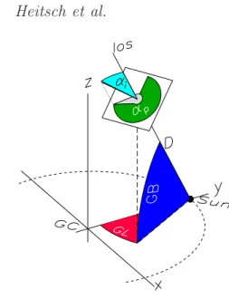
The coordinate system is set by the local (GL, GB) patch describing the plane-of-sky, and by the (unknown) cloud distance D along the line-of-sight (Fig. 1). The three-dimensional orientation of a CHVC requires two angles: The inclination angle 0 ≤αi ≤ π describes the angle between
the cloudtail and the line-of-sight, with the tail pointing away from the observer for αi = 0. The position angle
Figure 1.Definition of the coordinate system for CHVC orienta-tion. The position angleαp(green) and the inclination angleαi
(cyan) are defined in the local (GL,GB) patch, at an (unknown) distanceD from the Sun. A cartoon CHVC mapped within the local (GL,GB) patch is outlined in grey.
0 ≤ αp < 2π is counted counter-clockwise starting with
αp= 0 for the cloud’s tail pointing toward Galactic North.
The local coordinate patch is assumed to be rectangular – hence the limitation to CHVCs.
The goal is to relate the cloud shape in position-velocity space to the inclination angle. We demonstrate the process with the help of a simulation (Fig. 2) of a CHVC travel-ing atαi= 45◦toward the observer. The simulation (model
Wb1a15b ofHeitsch & Putman(2009), see their table 1 and fig. 2) is a wind-tunnel experiment, in which an initially spherical cloud of (in this case) radius 50 pc and density 0.1 cm−3 is exposed to a wind of 150 km s−1 and a density
of 10−5
cm−3
. The simulation generated∼30 3D data sets consisting of gas density, velocity and temperature. These are converted into position-position-velocity cubes by select-ing for gas with a temperature ofT <104
K (assumed to be neutral hydrogen), rotating by the desired inclination angle
αi0, and then calculating channel maps with ∆v= 1 km s−1
assuming optically thin HI-21 cm emission. Peak column densities reach ∼ 3×10¹⁹
cm−2
. These channel maps are then used for further analysis.
The position angleαp is determined by fitting ellipses
to the integrated intensity maps. Since the orientation of the ellipse is degenerate with π, we identify the tail of the cloud as the direction in which the cloud extends farthest from the column density peak (i.e. the location of the head). This assumes that the clouds have a head-tail structure. To estimate the inclination angle, we define the cloud’s ”back-bone” (i.e. the line through the cloud’s center-of-mass at the determinedαp), along which spectra are taken to construct
a position-velocity map (Fig. 2e-g). For a CHVC moving toward the observer, the (dense) core will appear at more negative velocities and the tail at more positive ones, hence the CHVC will be asymmetric along the velocity axis. Yet, along the position axis, the CHVC will appear more or less symmetric (Fig. 2d). If the CHVC moves perpendicularly to the line-of-sight, head and tail can be clearly identified,
Figure 2. (a) Integrated intensity, (b) centroid velocity, and (c) velocity dispersion of a model CHVC (model Wb1a15b of
Heitsch & Putman(2009)), traveling at 45◦to the observer. Con-tours are given at [1,5,9,13] K km s−1
. (d,e,f) Position-velocity plots for inclination anglesαi0= 0,45,90◦. Contours correspond to [5,15,25,35] K.
resulting in an asymmetry in position. Yet, the CHVC will appear symmetric in velocity space, since the gradient along the cloud backbone due to the differential drag will not be discernible, and only thermal and turbulent motions within the CHVC will contribute to the velocity signature (Fig.2f). A CHVC traveling at e.g. 45◦ to the observer will appear
asymmetric both in position and velocity (Fig.2e). We calculate the observable asymmetry of the CHVC’s gas distribution with respect to its center-of-mass. The asymmetry in position is given by
ap≡ ∆
2p−∆1p
∆1p+ ∆2p, (1)
with−1 ≤ap ≤ 1. The one-sided dispersions ∆1p,2p refer
to the CHVC extent to lower/higher values in position with respect to the center-of-mass, e.g.
∆1p=
X
p<pc,v
(p−pc)
2
T(p, v)
X
p<pc,v
T(p, v)
!1/2
, (2)
whereT(p, v) is the position-velocity map,pcis the
center-of-mass position, and the summation extends over allp < pc
(along the horizontal axis in Fig.2d-f), and over the whole velocity range. For ∆2p, the summation extends overp > pc.
The velocity extents ∆1v,2vare constructed similarly, along
the vertical (velocity) axis of the position-velocity plot. Other measures of cloud extent, such as 50% contours, give similar results. Since the accuracy of ∆1,2 depends on the
map resolution, spatial and velocity resolution of the tele-scope will affect the result. A CHVC with the tail pointing toward positivephasap>0, and a CHVC moving toward
3D Orientation of Compact HVCs
L3
asymmetries are normalized, and if we assume (to first or-der) a linear relationship between the velocity and the po-sition along the cloud’s tail (see e.g.Br¨uns et al. 2001), we can calculate the inclination angle as
αi= arctan
ap
av
. (3)
To test the method, position-position-velocity cubes are generated for the CHVC model of Fig.2, for a series of rota-tion anglesαi0. ”Spectra” (position-velocity plots) are taken
along the long axis of the cloud (Fig.2d-f), from which we derive the inclination angle estimateαi. Fig.3summarizes
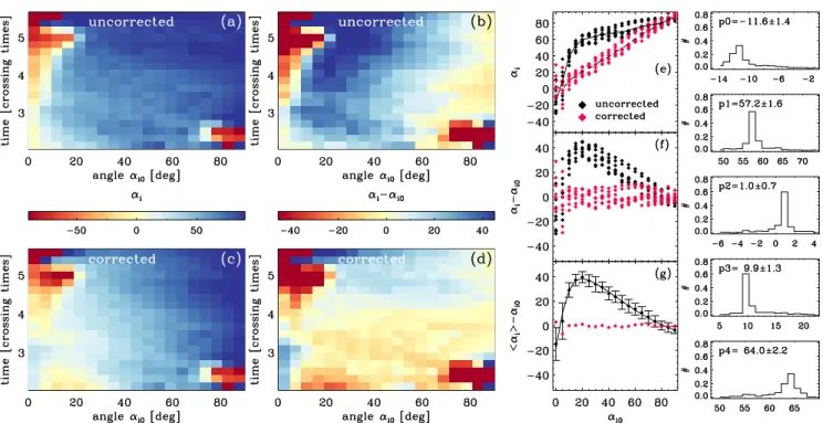
the reliability of the inclination angle estimates. Panels (a) and (b) showαi as derived from equation3, and its
resid-uals αi−αi0. Apart from occasional large deviations due
to substantial fractions of gas being stripped off the CHVC, the residuals depend systematically on the model rotation angle αi0 (Fig. 3f). Therefore, we attempt to improve on
equation 3 by fitting a heuristic function to the residuals; we average over the cloud evolution time (Fig.3g, the error bars are errors on the mean). The resulting corrected values are shown in red in Fig.3e through3g, and Fig.3b,d. The fitting function is given by
f(αi0) =p0tanh
αi0−p2
p3
expαi0−p2
p4
+p1. (4)
Parameter distributions and values derived from the Metropolis-Hastings algorithm used to fit equation 4 are given in the right column of Fig.3.
3 APPLICATION TO CHVCS
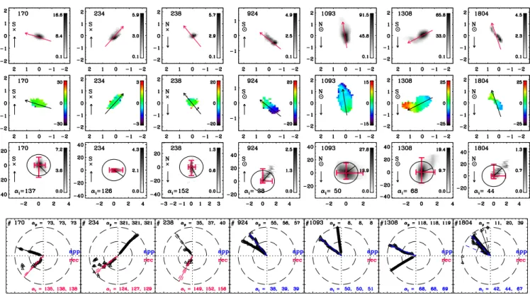
We apply the inclination angle estimate to selected CHVCs drawn from HIPASS (Putman et al. 2002). We select with a slight preference for head-tail clouds, yet we note that the head-tail structure would not show when the CHVC is traveling along the line-of-sight. The top two rows of Fig.4
show the integrated intensity and centroid velocity. HIPASS catalogue numbers are given in each panel. We apply a se-lection ellipse around the CHVC structure of interest, re-moving unassociated emission, both in (GL, GB)-space and invlsr-space.
We determine the angles αp and αi for a sequence of
increasing signal-to-noise values (S/N = [5,40] in steps of 1). For S/N <5, angle estimates were generally unreliable in our sample. The bottom row of Fig. 4 summarises the derived angles for the selected CHVCs. Shown are the me-dian values (solid lines) including lower and upper quartiles (dashed lines), to highlight the uncertainties in the angle estimates. The position angleαpcan be determined within
<±3◦(exception: cloud 1804, whose position angle “drifts” with S/N). For well-defined clouds, the inclination angles show similar ranges. To further assess the reliability of the angle estimates, we calculate αi for all 0 ≤αp ≤360 and
for allS/N. In the resulting map ofαi(αp, S/N) we search
for “consistent”αivalues, i.e. for regions in (αp, S/N) space
across whichαidoes not change by more than 2◦. These
re-gions are usually extended over a large range inS/N, while for inconsistent solutions, αi varies strongly with αp. The
largest of these regions is taken as the solution. The resulting angle estimates are consistent with the direct fits described above.
4 DISCUSSION
4.1 A Method to Constrain CHVC Distances
We explore whether the full cloud orientation can be used to derive distance constraints of CHVCs via the velocity of a CHVC relative to its background medium, vrel. This
re-quires several assumptions. It is not our intent that these be necessarily correct, but that they are sufficiently plausible to outline the method. The goal is to calculatevrel =|vtot−Θ|
along the line-of-sight at a given (GL, GB) for a range of distances D. Here, vtot is the three-dimensional velocity
of the CHVC in Galactic cartesian coordinates, and Θ is the three-dimensional (halo) rotation velocity of the back-ground medium. All velocities are relative to the Galactic Standard of Rest (GSR). Since vtot is constant along the line-of-sight, butΘ will change withD, vrel =vrel(D). If
we have additional information onvrel, such as a terminal
velocity vmax at which CHVCs can move with respect to
the background medium, distances D can be identified for whichvrel≤vmax.
SettingΘrequires a Galactic halo rotation model. For demonstration, we combine the rotation curve model of
Fich et al. (1989) with an exponential drop-off in z, re-producing the linear gradient of −22 km s−1
derived by
Levine et al.(2008). Our halo rotation model then reads as
|Θ| ≡vR(Rxy, z) = (109 + 108R
0.0042
xy )e−|z|/
10
, (5)
withRxy andz in kpc. The radius Rxy gives the
Galacto-centric distance in the plane, with the full GalactoGalacto-centric radius beingR= (R2
xy+z2)1/2.
There are several options to constrainvrel, such as
set-tingvmax to the terminal velocity due to hydrodynamical
drag (Benjamin & Danly 1997), estimating vrel based on
differential drag analysis of the CHVC (Peek et al. 2007), or limiting vmax to the sound speed of the background
medium for sufficiently diffuse CHVCs. Based on our mod-els (Heitsch & Putman 2009), we choose the latter and set
vmax=cs= 100 km s−1. Other options will be explored in
a future contribution.
Table 1 summarises the estimated parameters for the seven CHVCs shown in Fig. 4 together with a few other CHVCs selected from HIPASS. Roughly 50% of the sample CHVCs have near distance constraints (atcs= 100 km s−1).
Most remaining CHVCs show relative velocities vrel >
200 km s−1
, and thus do not lead to a distance constraint. The value of|vtot|depends strongly onαi: Atαi= 90,270◦,
|vtot|cannot be reconstructed.
Though none of the observed CHVCs have (previous) direct distance constraints, many of them are potentially re-lated to larger HVC complexes with constraints from their position-velocity proximity (Peek et al. 2008;Putman et al. 2011). In the Southern sky, the majority of the HVCs (and the CHVCs in Table 1) can be associated with the Mag-ellanic System and though the distance to the MagMag-ellanic complexes are unknown, the Magellanic Clouds themselves are at 50-60 kpc and the associated clouds are expected to be further away than the lower distance limits Dlo in
Figure 3.(a) Colour map of the uncorrected inclination angle estimate (equation3) depending on the rotation angleαi0, and on the model CHVC evolution time. Large “secular” differences occur when substantial fragments are stripped off the CHVC. (b) Uncorrected inclination angle residuals scaled between±45◦. (c) Corrected inclination angle estimates, and (d) corrected residuals. (e) Uncorrected (black) and corrected (red) inclination angles, and (f) their residuals. (g) Residuals calculated from averaged uncorrected inclination angle (black), empirical fit (line, see equation4), and resulting corrected residuals (red). The right column gives the fit parameter distributions and values.
Table 1.Selected HIPASS CHVC parameters. [1] HIPASS num-ber. [2] Galactic longitude GL. [3] Galactic latitude GB. [4] Po-sition angleαp. [5] Inclination angleαi. [6] Lower distance limit
Dlo. [7] Total velocity|vtot|. [8] Cloud approaching (⊙) or
reced-ing (⊗), and moving toward (↓) or away from (↑) disk. [9] Possible association with known HVC complexes. Complexes in square brackets do not have distance constraints. For identification of the HVC complexes, seeKalberla & Haud(2006);Putman et al.
(2012).
[1] [2] [3] [4] [5] [6] [7] [8] [9]
170 16.8 −25.0 73 138 − 240 ⊗ ↑ GCN
234 24.5 −1.8 321 127 − 324 ⊗ ↑ GCN
238 24.8 8.8 37 152 10.0 24 ⊗ ↓ C 924 258.5 −39.1 56 39 21.7 85 ⊙ ↑ LA 1093 271.0 10.8 8 50 20.9 72 ⊙ ↓ LA 1308 285.0 −16.1 118 68 22.4 2 ⊙ ↓ LA
1804 334.8 30.7 20 44 − 234 ⊙ ↓ L
48 3.9 −63.7 70 124 − 270 ⊗ ↑ MS?
200 21.2 −61.2 236 24 12.3 59 ⊙ ↓ MS? 632 224.1 −17.0 8 139 24.0 81 ⊗ ↑ MS? 648 226.6 −33.4 90 25 7.7 27 ⊙ ↑ MS? 1221 279.1 −16.7 211 49 8.4 97 ⊙ ↓ LA 1616 316.9 −76.8 94 67 − 166 ⊙ ↓ MS 1806 335.0 16.1 191 50 29.4 41 ⊙ ↑ [WD]
the results of the method are thus far consistent with exist-ing distance constraints.
The weakest link in these distance constraints is the choice of a halo rotation model. Increasing the characteristic scale from 10 to 20 kpc in equation5(and thus flattening the
drop-off ofΘwithz) increases all the distance constraints by a factor of∼2. Halo rotation models withoutz-dependence (Hodges-Kluck et al. 2016) do not yield resultsif we assume
vrel .100 km s−1. We interpret this as a limitation of our
assumptions regarding vrel rather than a limitation of the
method itself.
4.2 Caveats
Residual Fitting Correcting the inclination angle estimate (equation3) by fitting the residuals raises the question about the physical motivation for equation4. Equation3assumes that the velocity gradient along the tail, caused by decelera-tion of the cloud gas, is linear. This is not necessarily correct (Br¨uns et al. 2001;Peek et al. 2007, see also Fig. 2); mate-rial directly behind the cloud is expected to travel nearly at the same velocity as the cloud. Velocities close to the cloud speed reduce the velocity asymmetryav, thus overestimating
αi. The fit parameters might also depend on environmental
factors, such as the ambient density, and the absolute cloud velocity. These dependencies and their quantification can only be explored with a larger model grid, which is beyond the scope of this paper.
Effect of Background Flow on αi Since the CHVCs in our
sample are identified via HI emission, theirαiestimates rest
on the assumption that the neutral gas interacts directly with the background halo. Yet, there is evidence for sub-stantial ionized envelopes co-moving with HVCs (Hill et al. 2009; Lehner et al. 2009, 2012). For a CHVC moving at a velocity |vtot|=vrel+venv with respect to an ionized
3D Orientation of Compact HVCs
L5
Figure 4.Top to bottom: Integrated intensity for CHVCs selected from HIPASS (Putman et al. 2002), velocity centroid maps, position-velocity plots, and derived position and inclination angles. Red arrows denote the direction of the cloud tail. Positions in (GL, GB) are relative to the cloud’s catalogued coordinates. LettersNandSindicate Northern or Southern Galactic hemisphere. Black vertical arrows indicate whether the cloud is moving toward lower (downward) or higher|z|(upward). Clouds approaching the observer (αi<90◦) are
denoted by a dotted circle, otherwise by a “x”. The position axis in the pv-plots is counted from head to tail.Bottom row:Position angle
αp (black symbols, lines) and inclination angleαi (blue or red symbols, lines). Both anglesαp andαi are counted counter-clockwise
from the top, with 0≤αp≤360 and 0≤αi≤180. Long dashed circles indicateS/N values of 20 and 40. Solid lines refer to the median
value, short dashed lines to the lower and upper quartile. These values are given also at the top and bottom of each panel (lower quartile, median, upper quartile). The horizontal dashed line separates inclination angles for approaching (blue) and receding (red) CHVCs.
drag results in a smaller spread along the velocity axis in the position-velocity plot, and therefore in a pitch angle biased toward 90◦. This in turn increases the inferred total velocity
vtot. On the other hand, the observed radial velocity com-bines the line-of-sight component of the HI CHVC and the ionized envelope. Therefore, our method tends to overesti-mate|vtot|if the CHVC is moving within a larger ionized en-velope. Yet, if the line-of-sight component of the envelope’s velocity – and therefore the line-of-sight component ofvrel
– is known, the velocity spread in the position-velocity plot correctly refers to vrel, and thus αi is not affected by the
ionized envelope.
Effects of Cloud Evolution on αi The interaction of the
CHVC with the ambient gas leads to turbulent structures, and occasionally to large “chunks” of the cloud being ripped off. Such “secular” events can affect the estimates for αi
and αp. The strong time variations in the residuals of αi
(Fig.3b,d) are caused by this effect.
The αi estimate relies on the translation of the effect
of the hydrodynamic drag on the CHVC’s tail into centroid velocity profiles. The method assumes a monotonic centroid velocity profile, i.e. for a cloud moving at an angle toward the observer, the head would have the most negative veloc-ities, and the tail the most positive ones. Yet, the centroid velocity map of Fig.2 demonstrates that this need not be the case (alsoBr¨uns et al. 2001). The swath of “green” (less
negative) velocities at the head of the cloud is caused by material flowing around the cloud away from the observer.
5 SUMMARY
We present a method to determine the three-dimensional orientation of CHVCs. The inclination angle is derived from asymmetries in the intensity distribution of a CHVC’s position-velocity plot (Figs. 2and 4). We test the method with the help of numerical simulations of CHVCs and iden-tify possible systematic effects on the inclination angle es-timate. When applied to CHVCs drawn from HIPASS, the method is returning results that are stable with increasing signal-to-noise. The method can be improved by a more de-tailed analysis of the position-velocity plots, and by a more rigorous statistical treatment. Applications to clouds being ablated in other astrophysical environments seem obvious.
ACKNOWLEDGEMENTS
We thank the referee for a very thorough and concise report. This work was partially supported by UNC Chapel Hill, and it has made use of NASA’s Astrophysics Data System.
REFERENCES
Benjamin R. A., Danly L., 1997,ApJ,481, 764
Bland-Hawthorn J., Putman M. E., 2001, in Hibbard J. E., Rupen M., van Gorkom J. H., eds, Astronomical Society of the Pacific Conference Series Vol. 240, Gas and Galaxy Evolution. p. 369 (arXiv:astro-ph/0110043)
Br¨uns C., Kerp J., Kalberla P. M. W., Mebold U., 2000, A&A,
357, 120
Br¨uns C., Kerp J., Pagels A., 2001,A&A,370, L26
Fich M., Blitz L., Stark A. A., 1989,ApJ,342, 272
Fox A. J., et al., 2016,ApJ,816, L11
Heitsch F., Putman M. E., 2009,ApJ,698, 1485
Hill A. S., Haffner L. M., Reynolds R. J., 2009,ApJ,703, 1832
Hodges-Kluck E. J., Miller M. J., Bregman J. N., 2016, ApJ,
822, 21
Jin S., 2010,MNRAS,408, L85
Kalberla P. M. W., Haud U., 2006,A&A,455, 481
Lehner N., Staveley-Smith L., Howk J. C., 2009,ApJ,702, 940
Lehner N., Howk J. C., Thom C., Fox A. J., Tumlinson J., Tripp T. M., Meiring J. D., 2012,MNRAS,424, 2896
Levine E. S., Heiles C., Blitz L., 2008,ApJ,679, 1288
Lockman F. J., Benjamin R. A., Heroux A. J., Langston G. I., 2008,ApJ,679, L21
Olano C. A., 2008,A&A,485, 457
Peek J. E. G., Putman M. E., McKee C. F., Heiles C., Stan-imirovi´c S., 2007,ApJ,656, 907
Peek J. E. G., Putman M. E., Sommer-Larsen J., 2008, ApJ,
674, 227
Putman M. E., et al., 2002,AJ,123, 873
Putman M. E., Bland-Hawthorn J., Veilleux S., Gibson B. K., Freeman K. C., Maloney P. R., 2003,ApJ,597, 948
Putman M. E., Saul D. R., Mets E., 2011,MNRAS,418, 1575
Putman M. E., Peek J. E. G., Joung M. R., 2012, ARA&A,
50, 491
Richter P., de Boer K. S., Werner K., Rauch T., 2015, A&A,
584, L6
Saul D. R., et al., 2012,ApJ,758, 44
Stanimirovi´c S., et al., 2006,ApJ,653, 1210
Thom C., Putman M. E., Gibson B. K., Christlieb N., Flynn C., Beers T. C., Wilhelm R., Lee Y. S., 2006,ApJ,638, L97
Thom C., Peek J. E. G., Putman M. E., Heiles C., Peek K. M. G., Wilhelm R., 2008,ApJ,684, 364
Wakker B. P., 2001,ApJS,136, 463
Wakker B. P., van Woerden H., 1997,ARA&A,35, 217
Wakker B. P., et al., 2007,ApJ,670, L113