Projection based algorithms for variational inequalities

Projection Based Algorithms for Variational Inequalities

Sudhanshu Shekhar Singh

A thesis submitted to the faculty of the University of North Carolina at Chapel Hill in fulfillment of the requirements for the degree of Doctor of Philosophy in the Department of Statistics and Operations Research.

Chapel Hill 2010

Approved by

Shu Lu

Jon Tolle

David Rubin

Scott Provan

Abstract

SUDHANSHU SHEKHAR SINGH: Projection Based Algorithms for Variational Inequalities (Under the supervision of Dr. Shu lu)

Table of Contents

List of Tables . . . vi

1 Introduction . . . 1

1.1 Sources of variational inequalities . . . 2

1.2 Equivalent formulations . . . 7

1.2.1 Equation reformulations . . . 9

1.2.2 Merit functions . . . 11

1.3 Solution analysis . . . 12

2 Algorithms for variational inequalities . . . 16

2.1 Linear approximation based methods . . . 16

2.2 KKT based methods . . . 19

2.3 Proximal point method . . . 21

2.4 Projection based methods . . . 23

3 Two projection based algorithms . . . 32

3.1 An interior anchor point relaxed projection method . . . 32

3.2 A gap function based algorithm . . . 50

4.3 Numerical examples . . . 74

4.4 Conclusions . . . 76

Appendix . . . 78

List of Algorithms

2.1 Proximal point method for VIs . . . 23

2.2 He’s algorithm . . . 25

2.3 Hyperplane projection method . . . 27

2.4 Relaxed projection method for paramonotone VIs . . . 29

2.5 Zhu and Marcotte’s generic framework . . . 31

3.1 Interior anchor point RPM . . . 37

3.2 Descent algorithm . . . 54

3.3 Descent method for box constrained VIs . . . 61

CHAPTER 1

Introduction

Given a non-empty, closed and convex subset K ofRn and a mappingF fromK toRn, the

variational inequality problem VI(K,F) is to find a vectorx∗ ∈Ksuch that

hF(x∗), x−x∗i ≥0 ∀x∈K. (1.1)

The solution set of (1.1) is referred to as SOL(K,F). IfFis continuous, then SOL(K,F) is closed. Variational inequalities were introduced by Hartman and Stampacchia in 1966 for the study of partial differential equations with applications in the field of mechanics. Those variational inequal-ities were infinite dimensional. Finite dimensional VI theory was developed later in 1980 when Dafermos observed that traffic network equilibrium conditions have a structure of VI.

Variational inequalities provide a tool to formulate various equilibrium problems. Several well known problems, such as systems of nonlinear equations, first order conditions for linear and non-linear optimization problems, and complementarity problems, are special cases of variational in-equalities.

A geometric interpretation of a solution of VI(K,F) is thatx∗is a solution if and only ifF(x∗)

makes a non-obtuse angle with all the feasible directions going into K fromx∗. Alternately, we may say thatx∗ is a solution of VI(K,F) if and only if−F(x∗)is in the normal cone toKatx∗. The normal cone toKatx∈Kis defined as

N(K, x) ={d∈_Rn_{| hd, y−xi ≤0, ∀y∈K}. (1.2)}

factx∗ ∈int(K)implies thatx∗−τ F(x∗)∈int(K)for sufficiently smallτ. Hence (1.1) implies

hF(x∗),−F(x∗)i ≥0, that isF(x∗) = 0. In particular ifK =Rn, the solution set of (1.1) is the

same as that ofF(x) = 0.

1.1

Sources of variational inequalities

Complementarity problems

Variational inequalities are very closely related to complementarity problems (CP). WhenKis a cone, the VI assumes the form of a CP. For completeness, we introduce the definition of a CP. Given a coneK⊂_Rn_{and a mappingF :K→}

Rn, the complementarity problem, CP(K,F), is to

findx∈K such thatF(x)∈K∗and,

hx, F(x)i ≥0, (1.3)

whereK∗is the dual cone ofK defined as,

K∗={y∈_Rn_{| hy, xi ≥0, ∀x∈K}. (1.4)}

Two special cases of CP are very important:

(a) The nonlinear complementarity problem NCP(F): LetRn+denote the nonnegative othant ofRn,

and letF :Rn→Rn. The nonlinear complementarity problem (NCP) is to findx∗ ∈Rn+such

that

becauseF(x∗) ≥0,x ∈ _Rn

+andhF(x∗), x∗i = 0. On the other hand, ifx∗ ∈SOL(Rn+,F),

then (1.6) holds. Substitutingx= 0andx= 2x∗ in (1.6) implieshF(x∗), x∗i= 0. Moreover, substitutingx=eiin (1.6), whereeiis theithunit vector inRn, shows thatF(x∗)≥0.

(b) The mixed complementarity problem MiCP(G, H): LetGandHbe mappings fromRn1×Rn2+

toRn1 andRn2 respectively. The MiCP(G, H) is to find a pair of vectors(u, v)such thatv ≥0

and

G(u, v) = 0, hv, H(u, v)i= 0. (1.7)

System of equations

As already mentioned, solvingF(x) = 0is equivalent to solving VI(Rn,F). Hence any system

of equations can be considered as a variational inequality problem.

Optimization problems

Variational inequalities arise from various sources, constrained optimization problems being one of those. Consider the optimization problem,

min f(x), s.t. x∈K. (1.8)

Ifxis a local solution to this optimization problem, then the gradient of f atx must make a non obtuse angle with all the feasible directions going intoKfromx. This is precisely the definition of the VI withF =Of, that is, a local solutionxof (1.8) satisfies

hy−x,Of(x)i ≥0, ∀y∈K. (1.9)

But this does not imply that every VI can be rephrased as an optimization problem, because F : Rn → Rn is the gradient of some function if and only if the Jacobian ofF is symmetric. Hence

Saddle Point problems

LetL:Rn+m →Rbe an arbitrary function andX⊂RnandY ⊂Rmbe two closed sets. The

saddle point problem associated with (L, X, Y) is to find(x, y)∈X×Y such that

L(x, v)≤L(x, y)≤L(u, y), ∀(u, v)∈X×Y. (1.10)

IfLis convex onY for a fixedx, and concave onXfor a fixedy, then(x, y)solves the saddle point problem if and only if(x, y)solves the VI(X×Y,F) where

F = 

 

OuL(u, v)

−_OvL(u, v) 

 .

Nash equilibrium problems

Certain Nash equilibrium problems can be solved as variational inequalities. For example, con-sider the multiplayer noncooperative game withNplayers. LetKi ∈Rnibe the set of strategies that

playerican employ. Hereniis a positive integer. Each player has a cost functionθi(x1, x2, ..., xN) which depends on her own strategy and those of the other players. Given the strategies of the other players, playeriwants to determine a strategyyithat minimizesθi. So, the problem for playeriis

min θi(xi, xi) subject to xi∈Ki, (1.11)

wherexi_={x

j}j6=i. LetSi(x)be the solution set to (1.11). The Nash equilibrium is achieved at a collection of strategiesx={x_i}N

i=1such thatxi ∈Si(x).

produce so that each player maximizes her own profit.

Economic equilibrium models

Many economic activity models can be formulated as VI/CP. We will briefly explain the Wal-rasian equilibrium model, which predicts equilibrium activities and prices in an economy for which interactions between the commodities comprising this economy have been incorporated. Consider an economy withm economic activities and n goods. The unit cost of operating activityiis ci and the level of activityiis denoted byyi. The initial endowment for goodjisbj, its unit price is denoted bypj, and its demand function isdj(p)wherepis the vector of prices of all the goods.

The relation between the activity levels and the availability of goods is given by a technology input-output matrixA(p). Ais anm×nmatrix with entriesaij(p)such thathAT(p), yigives the vector of goods resulting from a vectory of activities; hA(p), pi is the vector of per unit activity returns. An activity price pair(y, p)is a general equilibrium if(y, p)≥0and

c− hA(p), pi ≥0

hy, c− hA(p), pii= 0,

b+hA(p)T, yi −d(p)≥0

hp, b+hA(p)T, yi −d(p)i= 0.

The first two conditions here mean that all activity levels are nonnegative, all activities give nonneg-ative profits, and activities with negnonneg-ative profits are not performed. The last two conditions state that the prices are non-negative, the supply must be at least as much as the demand, and supply exceeds demand only for free goods. These four conditions together define a complementarity problem.

Traffic equilibrium model

The traffic equilibrium model predicts the steady state traffic in a network in which all users are trying to use the network to minimize their travel cost. The sets of nodes and arcs of the network are denoted byN andArespectively. The flow on the network is given by a flow vector

functionca(f). There are two subsets,OandD, ofN, that are recognized as origin and destination sets respectively. The set of all origin-destination (OD) pairs is a subsetW ofO×D.

For an OD pairw∈W, letPwbe the set of all paths connectingwand letPbe the union of all paths for allw ∈ W. Lethp be the flow on pathp ∈ P andhbe the vector of path flows. Let us denote the travel cost on pathpasCp(h). Let∆be the arc path incidence matrix whose(a, p)entry is 1 if arca∈Ais on pathp∈P, and 0 otherwise. For eachw∈W, a functiondw(u)represents the demand for the OD pairwas a function ofu, the vector of minimum travel costs between all OD pairs.

The Wardrop user equilibrium principle postulates that users of the traffic network will choose minimum cost path between each OD pair, and through this process the paths that are used will have equal costs. Moreover, paths with costs higher than the minimum will have no flow. Also, the travel demand must be satisfied, and all the costs should be nonnegative. These conditions, written mathematically, state (Dafermos, 1980)

Cp(h)≤0, hp≥0

hCp(h)−uw, hpi ≥0, ∀w∈Wp∈Pw,

X

p∈Pw

hp =dw(u), ∀w∈W,

uw ≥0, ∀w∈W.

The static traffic user equilibrium problem is to find a pair(h, u)of path flows and minimum travel costs, so that the above conditions are satisfied. Under the assumption that the travel costs and demand functions are nonnegative, this is a complementarity problem.

This problem is closely related to semidefinite programs in which the unkowns are symmetric PSD matrices.

There are various other applications of VI and CP like frictional contact problems, elastoplastic structural analysis problems, nonlinear obstacle problems etc. For a detailed description of these problems, the reader is referred to Chapter 1 of the book (Facchinei and Pang, 2003).

1.2

Equivalent formulations

We can obtain equivalent formulations of VI (and CP) as systems of equations, optimization problem or fixed point problem. These formulations are helpful in developing analytical results and algorithms for solving VIs.

Let us define the functionFminas

Fmin(x) =min(x, F(x)) (1.13)

where themin(·,·)is a componentwise minimum operator. We can rewrite (1.13) as

Fmin(x) =x−ΠRn+(0

n_{, x−F(x)), (1.14)}

where0nis the origin inRnandΠRn+()is the Euclidean projection ontoR n

+. This formulation of

Fmin(x) leads to two equation reformulations of the VI. Both formulations require the projection operator. Since the projection operator plays a very important role in the study of VI, it is imperative that we define it formally and mention some of its elementary properties (Facchinei and Pang, 2003).

The projection of a pointy∈Rnon a closed convex subsetKofRn, denoted byΠK(y), is the pointx∈Kthat is closest toy. The problem of findingΠK(y)is the following

min 1

2hx−y, x−yi, subject tox∈K. (1.15)

unique solution. Moreover 1. for eachx∈_Rn_,Π

K(x)exists and is unique; 2. for eachx∈_Rn_,Π

K(x)is the unique vectory∈Ksatisfying

hz−y, y−xi ≥0, ∀z∈K; (1.16)

3. for any two vectorsuandvinRn,

hΠK(u)−ΠK(v), u−vi ≥ kΠK(u)−ΠK(v)k22; (1.17)

4. ΠK(x)is nonexpansive. That is, for any two vectorsuandvinRn,

kΠK(u)−ΠK(v)k2 ≤ ku−vk2; (1.18)

5. the squared distance function,

ρ(x) = 1

2kx−ΠK(x)k

2

2, x∈Rn, (1.19)

is continuously differentiable inRnwithOρ(x) =x−ΠK(x). Note that by the first order necessary conditions for (1.15), we have

hΠK(y)−y, x−ΠK(y)i ≥0, ∀x∈K. (1.20)

In addition to the Euclidean norm, we sometimes use a vector norm induced by a symmetric positive definite matrix to define a skewed projection operator. Given a positive definite matrix

D∈_Rn×n_{, theD-norm of a vectorx∈}

Rnis defined as

kxk_D =phx, Dxi. (1.22)

Then the skewed projectorΠK,D(x), of a vectorx, on a closed convex subsetKofRnis the solution

to

min 1

2hy−x, D(y−x)i,

s.t. y∈K. (1.23)

As in the case of euclidean norm, it follows from the first order conditions thatxsolves VI(K,

F) if it is the fixed point ofΠK,D(x−D−1F(x))and vice versa.

1.2.1 Equation reformulations

Two nonsmooth equation reformulations of VI(K,F) can be defined with the aid of the follow-ing maps,

F_Knat(x) =x−ΠK(x−F(x)), (1.24)

and

F_Knor(x) =F(ΠK(x)) +x−ΠK(x). (1.25)

These maps are referred to as the natural and normal maps associated with VI(K,F) respectively. The following proposition is a combination of Propositions 1.5.8 and 1.5.9 of (Facchinei and Pang, 2003).

Proposition 1.1. Let K⊂Rnbe closed and convex andF :Rn→Rnbe arbitrary. Then

1. x∈SOL(K, F)⇔F_Knat(x) = 0.

2. x∈SOL(K, F) if and only if there existszsuch thatx= ΠK(z)andFKnor(z) = 0.

(KKT) conditions for the problem. In order to be able to write the KKT conditions for VI(K,F), we assume that K can be specified as

K ={x∈Rn: g(x)≤0,

h(x) = 0}, (1.26)

whereg:Rn→Rmandh:Rn →Rlare continuously differentiable functions. Note thatx∈Rn

solves VI(K,F) if and only ifxis an optimal solution to the problem

minhF(x), y−xi, subject toy∈K.

Hence the KKT formulation for VI(K, F) is that for the aforementioned problem with x as the solution,

F(x) +hJ h(x)T, µi+hJ g(x)T, λi = 0,

h(x) = 0,

0 ≥ g(x)⊥λ ≥ 0, (1.27)

whereµ∈Rl,λ∈Rm are multipliers for the equality and inequality constraints respectively and J h(x), J g(x) are the Jacobian matrices for h andg respectively. To express (1.27) as a system of equations, we need to write the complementarity condition in an equality form. This can be achieved by using a C function.

VI(K,F) can be written as

φ(x, µ, λ) =            

L(x, µ, λ)

h(x)

CF(−g1(x), λ1)

.. .

CF(−gm(x), λm)

           

= 0, (1.28)

where CF is some C function, andL(x, µ, λ) = F(x) +hJ h(x)T, µi+hJ g(x)T, λi is the La-grangian function. An example of a C function is themin(·,·)function.

1.2.2 Merit functions

A merit function for a problem is a nonnegative function that takes a zero value only for the arguments that solve the problem. Formally, a merit function for VI(K,F) is defined as follows. Definition 1.2. A merit function for VI(K,F) on a closed setX ⊇ K is a nonnegative function

θ:X→_R+such thatx∈SOL(K, F)⇔x∈Xandθ(x) = 0. In other wordsx∈SOL(K, F) if and only ifxsolves

min θ(y), y ∈X (1.29)

with the optimal objective value equal to 0.

A natural merit function, called the gap function, arises from the definition of VI(K,F). This function is defined on the domainDofF, and is given by

θgap(x) = sup y∈K

hF(x), x−yi, x∈D⊇K. (1.30)

This is clearly a nonnegative extended value function onK. SinceKis closed, findingθgap(x)is a concave maximization problem with a linear objective. Note that in general, this gap function is not differentiable, even in the simple case when the setKis polyhedral.

not guarantee to find the global minima. In general there must be some conditions on VI(K,F) in order for the stationary point of the gap function to be a solution to VI(K,F).

1.3

Solution analysis

We have already seen how VIs are related to optimization problems and the problem of solving a system of nonlinear equations. We also observed how a VI can be reformulated as a system of equations and/or a minimization problem. Results from analysis of such systems can then be applied to obtain the existence and uniqueness results of solutions to VI. In this section, we introduce several results on existence of the solution of a VI. These are well known results. We present them here and include their proofs for the sake of completeness. Interested reader is referred to (Facchinei and Pang, 2003)

Theorem 1.2. IfK is compact and convex andF is continuous onK, then VI(K,F) has at least one solution.

Proof. According to Brouwer’s fixed point theorem, for a continuous mapP : K → K, there is at least onex∗ ∈K such thatP(x∗) =x∗. Due to the continuity ofF,I−τ F is continuous for

τ >0. The projection operatorΠK(x)is also continuous. Hence their compositionΠK(x−F(x)) is also continuous. The conclusion follows from compactness ofK and the fact that a solution of

V I(K, F)is a fixed point of the mapΠK(x−F(x)).

If the feasible setK is not compact, the fixed point theorem is not applicable, but a solution to VI(K,F) exists under conditions given in the following theorem. LetBR(0)denote a closed ball of radiusRcentered at the origin and letKR=K∩BR(0).

Clearly,kyk> R. That is, the directiony−x∗

Rmakes an obtuse angle withF(x∗R). Letz=β(y−x) withβ >0such thatkx∗_R+zk< R. We can find such aβ >0sincekx∗_Rk< R. Due to convexity ofK,x∗_R+zbelongs to K and hence toKR. We have

hF(x∗_R), z−x∗_Ri=hF(x∗_R), zi=hF(x∗_R), β(y−x)i=βhF(x∗_R),(y−x)i<0.

The last inequality follows from (1.31). This contradicts with the assumption thatx∗_Rsolves VI(KR,

F).

Corollary 1.4. Suppose thatF is coercive. That is, there existsx0∈K, such that

hF(x)−F(x0), x−x0i kx−x0k

→ ∞ (1.32)

askxk → ∞forx∈K. Then VI(K,F) has a solution.

Uniqueness and existence results for VI(K,F) can be easily proven under various monotonicity assumptions. The following notions of monotonicity play important roles for analysing VIs. Let

K ⊂_Rn_{, and letF :K →}

Rn. ThenF is said to be

(a) strongly monotone onKwith constantτ >0if for each pair of pointsu, v∈K, we have

hF(u)−F(v), u−vi ≥τku−vk2;

(b) ξ monotone for someξ >1onKwith constantτ >0if for each pair of pointsu, v∈K, we have

hF(u)−F(v), u−vi ≥τku−vkξ;

(c) strictly monotone onKif for each pair of pointsu, v∈K,u6=vwe have

hF(u)−F(v), u−vi>0;

(d) monotone onKif for each pair of pointsu, v∈K, we have

(e) pseudomonotone onKif for each pair of pointsu, v∈K, we have

hF(v), u−vi ≥0⇒ hF(u), u−vi ≥0;

(f) quasimonotone onKif for each pair of pointsu, v∈K, we have

hF(v), u−vi>0⇒ hF(u), u−vi ≥0;

(g) explicitly quasimonotone onK if for all distinctu, v∈K, the following holds,

hF(v), u−vi ≥0⇒ hF(z), u−vi>0 for somez∈(0.5(u+v), u).

It follows from the definitions that (a)⇒(b)⇒(c)⇒(d)⇒(e)⇒(f), and (g)⇒(f).

The following results demonstrate that ifF has certain monotonicity properties, the solution set to the VI possesses certain desirable characteristics.

Theorem 1.5. LetK ⊂ _Rn _{be closed and convex, and F : K →}

Rn be continuous. Then the

following hold.

(a) IfF is strictly monotone onK, then there is at most one solution to VI(K, F).

(b) IfF isξmonotone for someξ >1, then VI(K,F) has a unique solution.

The proof of (a) follows by the definition of VI and strict monotonicity. (b) follows from the fact thatξ monotonicity implies coercivity. Strict monotonicity does not guarantee existence of a solution to VI. Pseudo monotonicity ofFgives the following result.

Theorem 1.6. Let K⊂_Rn_{be closed and convex, andF :K →}

If in addition to being strongly monotne, F(x) is also strongly Lipschitz continuous, then

CHAPTER 2

Algorithms for variational inequalities

The algorithms for solving VI(K,F) can be classified into several categories depending upon which formulation a method exploits. There are methods based on KKT conditions, gap/merit functions, interior and smoothing methods, and projection based methods.

The algorithms for solving variational inequalities can also be categorized based on the sub-problems that are solved in each iteration. A general approach to solving VI(K, F) consists of creating a sequence{xk_{} ⊂K such that eachx}k+1_{solves VI(K,F}k_),

hFk(xk+1), y−xk+1i ≥0 ∀y∈K, (2.1)

whereFk(·)is some approximation toF(x).Fkcan be linear or nonlinear.

2.1

Linear approximation based methods

A linearFkis of the form

4. Successive over relaxation: A(xk) = T(xk) + D_ω(x∗k), where T(xk) is the upper or lower

triangular part ofOF(xk)andω∗is a parameter in (0, 2). 5. Symmetrized Newton:A(xk) = 1₂{_OF(xk) +OF(xk)T}.

6. Projection method: A(xk) =G, a symmetric positive definite matrix.

The convergence of these methods depends onx∗being a regular solution to VI(K,F).

Definition 2.1. (Robinson, 1980) Letx∗ be a solution to VI(K,F), andF be differentiable atx∗. Thenx∗ is called a regular solution if there exists a neighborhoodN ofx∗and a scalarδ >0such that for everyywithkyk2 < δ, there is a unique vectorx(y)∈N, Lispchitz continuous with respect

toy, that solves the perturbed linearized VI(K,Fy) withFy :Rn→Rndefined as

Fy(x) =F(x∗) +y+h_OF(x∗), x−x∗i. (2.3)

Let the setKbe defined as in (1.26) withgi,hjbeing twice continuously differentaible for each

iandj, andF being once continuously differentiable. Letx∗ ∈SOL(K, F). Suppose that the following conditions hold.

1. There exist vectorsµ∗∈_Rl_{, andλ}∗ _∈

Rm, such that(x∗, µ∗, λ∗)satisfy the KKT conditions

for VI(K,F).

2. Linear independence constraint qualification (LICQ) holds atx∗. That is, the vectors{_Ogi(x∗) :

i ∈ I+∪I0, Ohj(x∗)}are linearly independent, whereI+ = {i : λ∗i > 0} andI0 ={i:

gi(x∗) = 0, λ∗_i = 0}. 3. The second order condition

hz,[OF(x∗) +

l

X

i=1

µ∗_iOh2_i(x∗) +

m

X

i=1

λ∗_iOg_i2(x∗)]zi>0 (2.4)

holds for allz6= 0such that,

hz,_Ogi(x∗)i= 0 ∀i∈I+,

Thenx∗ is a regular solution to VI(K,F) (Robinson, 1980). If x∗ is a regular solution to VI(K,

F), then there exists a neighborhoodN ofx∗ such that Newton’s method converges tox∗as long as it starts from an initial pointx0 ∈ N (Josephy, 1979b). Furthermore, ifOF(x∗) is Lipschitz continuous around x∗, then the convergence rate is quadratic. But Newton’s method for solving VI(K,F) suffers from the following drawbacks.

1. OF(x∗)needs to be evaluated at every step.

2. Each iteration requires solving a variational inequality subproblem.

3. The method converges only if the initial iterate is close enough to a solution.

Quasi Newton methods overcome the first drawback of Newton’s method. For instance, secant methods (Josephy, 1979a) update the matrixA(xk_{)in each iteration by a simple small rank matrix.} Although this reduces the work of findingOF(xk) at each iteration, it does not make solving the subproblems any easier. Those methods can achieve a superlinear convergence rate at best.

Other linear approximation methods, including the linearized Jacobi method, symmetrized New-ton method and projection algorithms, use a symmetric matrixA(xk)at each step. In these methods, the subproblem can be formulated as an optimization problem, thereby making it amenable to var-ious optimization lagorithms. On the downside, those methods require stronger restrictions on the problem, and do not have quadratic rate of convergence. The linearized successive over relaxation method solves an LCP with a triangular matrix at each step. The following theorem summarizes the performance of the linearized Jacobi method and the symmetrized Newton’s method.

Theorem 2.1. (Chan and Pang, 1982) LetK be a nonempty, closed and convex subset of_Rnand letF be a function fromRntoRn.

1. Suppose that F is once continuously differentiable, x∗ solves VI(K, F) and _OF(x∗) has

neighborhood.

2. Suppose thatF is once continuously differentiable,x∗solves VI(K,F), and thatOF(x∗)is

positive definite. LetA(x∗)andC(x∗)be the symmetric and skew symmetric parts ofOF(x∗)

respectively. If

kC(x∗)k₂ < λmin(A(x∗)), (2.6)

whereλmin(A(x∗))denotes the least eigenvalue ofA(x∗), then there exists a neighborhood ofx∗ such that the sequence generated by the symmetrized Newton method is well defined

and converges tox∗if it starts with an initial point within that neighborhood.

Moreover, the convergence rate of each of these methods is geometric, that is, there exists a constant

r∈(0,1)such that for a certain vector norm and for allk,

kxk+1−x∗k ≤rkxk−x∗k holds.

A class of methods applicable to VI(K,F) whenK is a compact polyhedral set are the simpli-cial decomposition methods. SinceK is a compact polyhedron, it can be expressed as the convex hull of its extreme points. At iterationk, a VI(Kk_,Fk_{) is solved, whereK}k_{denotes the convex hull} of a subset of extreme points ofK. A merit function is used to decide upon the addition or deletion of extreme points fromKkto obtainKk+1. The effectiveness of the method depends on how many extreme pointsKhas, and on the merit function used to guide the choice of extreme points at each iteration. (Lawphongpanich and Hearn, 1984) shows that if the gap functionminy∈KhF(x), y−xi is used to controlKk, andFk=F for all iterations, then the method terminates in a finite number of major iterations ifF is strongly monotone.

In what follows, we briefly describe methods based on the KKT formulations of variational inequalities, and proximal point methods.

2.2

KKT based methods

Fischer-Burmeister (FB) C-function,

ψF B(a, b) =

p

a2_+b2_{−(a+b), ∀(a, b)∈R}2_,

we can obtain two different equation reformulations for VI(K,F). Let

φF B(x, µ, λ) =

           

L(x, µ, λ)

h(x)

CF B(−g1(x), λ1)

.. .

CF B(−gm(x), λm)

            ,

φmin(x, µ, λ) =

           

L(x, µ, λ)

h(x)

min(−g1(x), λ1)

.. .

min(−gm(x), λm)

            .

A natural merit function for the KKT formulation is

θ(x, µ, λ) = 1

2hφ(x, µ, λ), φ(x, µ, λ)i,

whereφ(x, µ, λ)can be eitherφF B(x, µ, λ)orφmin(x, µ, λ). One can then try to solve the equation

φ(x, µ, λ) = 0, or to minimizeθ(x, µ, λ). Algorithms based on the merit functionθ(x, µ, λ)can be regarded as special cases of interior point methods which use a more generic potential function

2.3

Proximal point method

The proximal point method is another class of solution methods for VIs. This method solves VI(K, F +kI) at iterationk. Here {k} is a sequence of positive scalars going to zero, and I is the identity map. IfF is monotone, thenF +I is strongly monotone. Thus each subproblem has a unique solution. (Rockafellar, 1976) showed that ifkare chosen according to an appropriate inexact rule, then the sequence{xk_{}is bounded if and only if SOL(K,F) 6=φ. Moreover, if the} sequence{xk_{}is bounded, then it converges to a solution of VI(K,F).}

In the following generic proximal point scheme, VI(K,Fc,x), whereFc,x(y) =y−x+cF(y) is solved inexactly at each iteration. The algorithm uses the fact that ifF is monotone then the set valued map F +N(K,·) is maximal monotone. A set valued map φ : Rn → Rn is (strongly)

monotone if there exists a constantc(>)≥0such that

hx−y, u−vi ≥ckx−yk2 _{∀x, y∈dom(φ)andu∈φ(x), v∈φ(y). (2.7)}

A monotone mapφis maximal monotone if no monotone mapψexists such thatgraph φ⊂graph ψ. The following properties of maximal monotone maps ((Facchinei and Pang, 2003)) play an important role in the development of the algorithm being described here.

Theorem 2.2. Let a set-valued mapφ : Rn → Rn be given. Then the following statements are

equivalent.

1. φis maximal monotone.

2. φis maximal monotone and range(I+φ) =Rn.

3. For any positivec,(I+cφ)−1is 1-co-coercive and dom(I+cφ)−1 =Rn.

4. For any positivec,(I+cφ)−1is non-expansive and dom(I+cφ)−1 =Rn.

The map(I+cφ)−1 _{is called the resolvent ofφ, with constant c, and is denoted byJc,φ. It is}

single-valued and non expansive for a monotoneφ, and its domain isRnifφis maximal monotone.

Proposition 2.3. For a maximal monotoneφ, every positive c, andx∈_Rn_{,0∈φ(x)if and only if}

Jc,φ(x) =x.

Proposition 2.4. LetK ⊂_Rn_{be nonempty closed and convex andF :K →}

Rncontinuous. Then

the following hold forT ≡F+N(K,·).

1. Jc,T(x) =SOL(K,Fc,x), whereFc,x ≡y−x+cF(y).

2. N(K,·)is maximal monotone.

3. IfF is monotone thenT is maximal monotone.

If a maximal monotone mapT has a zero, it can be obtained by using a fixed point recursion on the resolvent ofT. Finding the resolvent is often a non-trivial problem itself. For instance, finding the resolvent to solve VI(K,F) is equivalent to solving VI(K,I−x+F). The following theorem states that finding the exact resolvent in the fixed point iteration is not necessary.

Theorem 2.5. LetT :Rn →Rnbe a maximal monotone map and letx0 ∈Rnbe given. IfT has

a zero, the sequence defined by

xk+1 =xk+ρk(wk−xk), (2.8)

where, for all k,

kwk_−J ck,T(x

k_{)k ≤}

k (2.9)

and {_k} ⊂ [0,∞] satisfies P

k < ∞, ρk ⊂ [Rm, RM], where 0 < Rm ≤ RM < 2, and

ck⊂(Cm,∞), whereCm >0, converges to it.

Algorithm 2.1Proximal point method for VIs Initialization: Choose x0 ∈ _Rn_{, c}

0 > 0, sequences {k}, {ρk}, and{ck} as required by the previous theorem. Setk= 1, loop =0.

whileloop = 0do

ifxk∈SOL(K,F)then Set loop= 1.

else

Findwksuch thatkwk−JckT(x

k_{)k ≤k.}

Setxk+1 =xk+ρk(wk−xk), Setk=k+ 1.

Selectck,k, andρk. end if

end while

If the VI has a solution, the algorithm converges to it. Otherwise the sequence generated by the algorithm is unbounded.

2.4

Projection based methods

We observed thatxsolves VI(K,F) if and only if

x= ΠK,D(x−D−1F(x)) (2.10)

where ΠK,D is the skewed projector onto K defined by a n×n positive definite matrix D. If the projection map defined in (2.10) is a contraction, the sequence {x_k}∞

k=0 defined as xk+1 =

ΠK,D(xk−D−1F(xk))converges to its fixed point irrespective of the choice ofx0.

Theorem 2.6. ((Facchinei and Pang, 2003)) LetK be a closed and convex subset ofRnandF : K →_Rn_{beµmonotone and Lipschitz continuous with constantL. If}

then the mappingΠK,D(x−D−1F(x))is a contraction from K to K with respect to the norm

k · k_D. Moreover, the sequence{xk_{}generated by the iterations}

xk+1= ΠK,D(xk−D−1F(xk)), (2.12)

starting from anyx0 ∈ K, converges to the solution of the VI(K,F) with a linear rate of

conver-gence.

One issue with the standard projection method is that it requires knowledge of constants charac-terizing Lipschitz continuity and strong monotonicity. The extragradient method requires a slightly weaker assumption onF, that is,F needs to be pseudomonotone. It requires two pojection calcula-tions in each iteration:

xk+1/2 = ΠK(xk−τ F(xk)),

xk+1 = ΠK(xk−τ F(xk+1/2)).

The extragradient method still requires knowledge of the Lipschitz constant, L, of F, since it converges only if τ < L. Due to the pseudo monotonicty of F, the hyperplane {x ∈ _Rn _:

hF(xk+1/2),(x−xk+1/2)i= 0}separatesxkfrom any solutionx∗. Consequentlyxk+1 is a move fromxkin a direction pointing towards SOL(K,F).

A projection based method by (He, 1997) uses the (2.10) formulation of a VI with D = βI, whereβis a positive scalar. This algorithm requiresF to be monotone. Define

e(u, β) = u−ΠK[u−βF(u)],

Algorithm 2.2He’s algorithm

Initialization: Chooseγ ∈ (0,2), α, δ ∈ (0,1)andβ > 0. Choose an arbitraryx0 ∈ K. Set

k= 1, loop= 0. whileloop = 0do

ifxk∈SOL(K,F)then Set loop= 1.

else

Setβk =β.

whilee(xk, βk)Td(xk, βk)< δke(xk, βk)k2do

βk:=αβk. end while Setβ =βk.

Setg(xk, β) =G−1d(xk, β). Setρ(xk, β) = e(x_kk_g,β_(x)Tk_,βd(₎x_kk2,β). Setxk+1 =xk−γρ(xk, β)g(xk, β)

Setk=k+ 1

end if end while

Because the sequence{xk_{}generated by any contraction method is bounded and the mapping} F is continuous, it is possible to prove that there is aβmin >0such that, for allk, βk ≤βminand the method with Armijo’s linesearch is well defined.

The hyperplane projection algorithm requires an even milder assumption on F, that of being pseudo monotone. The algorithm can be described as follows. Letτ > 0be a fixed scalar. Let

xk ∈Kbe given. First computeΠK(xk−τ F(xk)); call ityk. Now search the line segment joining

xkandykfor a pointzksuch that the hyperplane

Algorithm 2.3Hyperplane projection method

Initialization: Choosex0∈K,τ >0, andσ∈(0,1). Setk= 1. loop =0. whileloop = 0do

ifxk∈SOL(K,F)then Set loop= 1.

else

Setyk= ΠK(xk−τ F(xk)).

Find the smallest non negative integeriksuch that

hF(2−iyk+ (1−2−i)xk), xk−yki ≥σ τkx

k_−yk_k2_{. (2.14)}

Set

zk= 2−ik_yk_{+ (1−2}−ik_)xk

Set

wk= Π_Hk(xk) =xk−

hF(zk_{), x}k_−zk_i

kF(zk_)k2 F(z

k₎

Setxk+1 = ΠK(wk).

k=k+ 1

end if end while

The common drawback with the methods described above is that they all require computation of projection onK, which is often not an easy task to perform. A method described by Fukushima (Fukushima, 1986) simplifies this task by taking projection on a half space containingK. He makes the following assumptions.

2. F is strongly monotone on an open set containingK.

3. For somez∈K, there exists aβ >0, and a bounded setD⊂_Rn_{such that}

hF(x), x−zi ≥βkF(x)k2 ∀x /∈D. (2.15)

4. The setK ={x ∈_Rn _{|c(x) ≤0}, wherec:}

Rn →Ris convex and the Slater condition is

satisfied.

5. For anyx∈_Rn_{, at least one subgradientd∈∂c(x)can be calculated, where∂c(x) ={g∈}

Rn|c(y)≥c(x) +hg, y−xi ∀y∈Rn}.

Fukushima’s method is to take the projection ofxk−ρkG−1 F(x

k₎

kF(xk_)k

2 on the halfspaceT

k_defined as

Tk={x∈_Rn_|c(xk_{) +hg}k_{, x−x}k_{i ≤0} (2.16)}

where{ρ_k}is a sequence of positive parameters satisfyinglimk→∞ρk = 0and

P∞

k=1ρk = ∞. This algorithm does not require the starting point to be feasible. In fact, the intermediate solutions could also be infeasible in this method. The assumption (3.13), which is not satisfied by many VI problems, is crucial for convergence of this algorithm.

Algorithm 2.4Relaxed projection method for paramonotone VIs Initialization: choosex0∈K, and a sequence{β_k}, such thatP

βk=∞, andPβk2<∞. Set

k= 1, loop =0. whileloop = 0do

ifxk∈SOL(K,F)then Set loop= 1.

else

Setηk= max{1,kF(xk)k}. Setxk+1 = Π_Tk(xk−β_ηk

kF(x

k_)). Setk=k+ 1

end if end while

A generic gap function based framework given by (Zhu and Marcotte, 1994) encompasses sev-eral methods for solving monotone VIs. LetΩ(y, x) :K×K → _Rbe non-negative, continuously differentiable onK×K, strongly convex onKwith respect toyfor allx∈Kand satisfy

Ω(x, x) = 0andOyΩ(x, x) = 0 ∀x∈K. (2.17)

Define

h(y, x) =hF(x), x−yi −Ω(y, x), (2.18)

g(x) = max

y∈Kh(y, x) =h(H(x), x), (2.19) whereH(x)is the unique maximizer ofh(y, x)overK.

Sinceh(x, x) = 0, one always hasg(x) ≥ 0. Ifxsolves VI(K,F), thenh(y, x) ≤0implies

g(x) = 0. Conversely, if g(x) = 0, then x solves max

inequality formulation of the problem of findingH(x)is

h_Oyh(x, x), z−yi ≥0 ∀z∈K

i.e,hF(x), z−yi+h_OyΩ(x, x), z−yi ≥0 ∀z∈K i.e,hF(x), z−yi ≥0 ∀z∈K,

sinceOyΩ(x, x) = 0. Henceg(v)is a valid gap function for VI(K,F).

The problem of findingH(x)is equivalent to solving the following auxiliary VI (AV I(x))

hF(x) +OuΩ(y, x), w−yi ≥0 ∀w∈K. (2.20)

Note thatgis differentiable with gradient given by

Og(x) =F(x) +h_OF(x),(x−H(x))i −_OyΩ(H(x), x). (2.21)

Under the assumptions thatF(x)is strongly monotone andΩsatisfies

h_OyΩ(y, x) +OxΩ(y, x), y−xi ≥0 ∀y, x∈K, (2.22)

Algorithm 2.5Zhu and Marcotte’s generic framework

Initialization: choosex0 ∈K, andγ, β, σin(0,1). Setk= 1, loop =0. whileloop = 0do

ifxk∈SOL(K,F)then Set loop= 1.

else

SolveAV I(xk)forH(xk). Setdk_=H(xk_)−xk_. ifg(xk+dk)< γg(xk)then

Setxk+1=xk+dk=H(xk). else

Select the smallest integermsuch that

g(xk)−g(xk+βmdk)≥ −σβmhOg(xk), dki,

Setxk+1=xk+βmdk. Setk=k+ 1

end if end if end while

IfΩis chosen carefully, then theAV Iis easier to solve than the VI. The choiceΩ = 0leads to an algorithm with the function (1.30) as the gap function. The choiceΩ(y, x) =hy−x, G(y−x)i

CHAPTER 3

Two projection based algorithms

This chapter proposes two algorithms for solution of variational inequalities. Both of them be-long to the broad category of projection based algorithms. The goal in developing these algorithms is twofold. First, the algorithms should converge under mild conditions, to be applicable to a gen-eral class of problems. Second, the subproblems in the iterations should be easy to solve. To this end, we present in Section 3.1 a modified relaxed projection based algorithm, which generates the halfspaces that are close to the boundary of the original set, using an anchor point. Halfspaces generated in such a way provide better approximations of the original set comparing to halfspaces generated by the iterate points, and therefore lead to fewer iterations in solution of variational in-equalities. Section 3.2 presents a gap function based algorithm, which fits in the general framework introduced in (Zhu and Marcotte, 1994), with the special feature that the subproblems are solvable by relaxed projection methods. In section 3.3, we present an application of the descent framework to the oligopoly problem. The application leads to a special algorithm for box constrained variational inequalities, which requires taking projections on the box, and does not require knowledge of the monotonicity or Lipschitz constant of the functionF.

the boundary of the set. Halfspaces generated by such support points provide better approximations of the original set. However, it is not possible to find the exact support points due to computational errors. Thus, in real implementation of such methods, one has to use an estimated support point. This section studies a method, which we call the interior anchor point relaxed projection method (IAPRPM), in which an estimated support point is found via a binary search. We prove that the algorithm still converges, and test the algorithm with numerical examples.

In order for the IAPRPM to converge, we make the following assumptions. Among these, K1, K2, F1 and F2 are assumed throughout this section. Assumption F3 will be used in proofs of some results.

Assumption K1. The defining set,K, is given as

K ={x∈_Rn|c(x)≤0}, (3.1)

wherec:Rn→Ris a convex function.

Assumption K2. There exists a pointy¯such thatc(¯y)<0(Slater condition). Assumption F1. The functionF is continuous on an open set containingK.

Assumption F2. The functionF is strongly monotone on an open set containingK. Assumption F3. There exist az∈K,β >0, and a bounded setD⊂_Rn_{such that}

hF(x), x−zi ≥βkF(x)k₂ ∀x /∈D. (3.2)

Note that ifKis specified as

K ={x∈_Rn|ci(x)≤0i= 1, . . . , r}, (3.3)

we can definecasc(x) = min

i=1,...,rci(x). For eachx∈_Rn_{, we define}

whereg∈δc(x), the set of subgradients ofc(x). The setδc(x)is defined as

δc(x) ={g∈Rn|c(y)≥c(x) +hg, y−xi, ∀y∈Rn}. (3.5)

Note that, strictly speaking, the aboveH(x)should be replaced asH(x, g), as it depends not only on x but also on the arbitrarily chosen subgradientg. However, for notational convenience we write it asH(x), and adopt the convention that for eachxa single subgradient is selected. In what follows, we present some preliminary results that stem from convexity of K, followed by a description of the IAPRPM algorithm and the proof of its covegrence.

Lemma 3.1. Letx∈_Rn_{, and define the half space}

H−(x) ={y ∈_Rn_{|c(x) +hg, y−xi ≤0},}

wheregis a subgradient ofKatx. ThenK ⊂H−(x).

Proof. Lety∈K. Thenc(y)≤0. By the definition of subgradient, we have

c(x) +hg, y−xi ≤c(y).

Hencey∈H−(x).

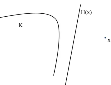
Lemma 3.2. Letx∈Rnwithc(x)>0. Then the hyperplaneH(x)strictly separatesxfromK.

Proof. Eachs∈Ksatisfies

c(x) +hg, s−yi ≤c(s)≤0.

Figure 3.1:H(x)strictly separatesxfromK

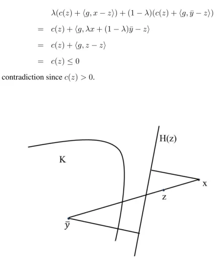
Proposition 3.3. Letx /∈ K, and lety¯be the point in assumption K2. LetLbe the line segment joiningxandy¯. Ifz∈L\K, thenH−(z)containsK, andH(z)separatesxfromKstrictly.

Proof. ThatH−(z)containsKfollows directly from Lemma 3.1.

By Lemma 3.2,z /∈H−(z). Sincez ∈L\K, we can assume thatzis a convex combination ofxandy¯. That is,

z=λx+ (1−λ)¯y

for someλ∈(0,1). Ifx∈H−(z), then we have

c(z) +hg, x−zi ≤0

and

c(z) +hg,y¯−zi ≤0

λ(c(z) +hg, x−zi) + (1−λ)(c(z) +hg,y¯−zi)

= c(z) +hg, λx+ (1−λ)¯y−zi

= c(z) +hg, z−zi

= c(z)≤0

which is a contradiction sincec(z)>0.

Figure 3.2:H(z)separatesxfromK

Algorithm 3.1Interior anchor point RPM

Initialization: Selectx0 ∈Rn, a small > 0, a sequence{ρk}withρk → 0, and

∞ X

k=1

ρk = ∞

and a positive definite matrixG. Setk= 1, loop= 0. whileloop = 0do

Find the point to be projected as

pk=   

 

xk−ρkG−1 F(x

k₎

kF(xk_)k

2 ifF(x k_{)6= 0}

xk ifF(xk) = 0.

ifxk_∈Kthen

setxk+1= Π_H−_(xk_),G(pk).

else

Construct the line segmentLk fromy¯toxk. Find a pointwk onLk with c(wk) > 0and

dist(wk, K)≤kvia a binary serach betweenxkandy¯. Setxk+1 = Π_H−_(wk_),G(pk).

end if

ifxk+1 =xkthen set loop= 0. end if

setk=k+ 1. end while

Algorithm 3.1 involves finding the skewed projection of a point on a halfspaceS, which has a closed form formula. Let a halfspaceSbe of the form,

S={x∈_Rn|hg, xi ≤c}. (3.6)

ΠS,G(p)are

G(y−p) +µg= 0, (3.7)

hg, yi ≤c,

µ×(hg, xi −c) = 0,

µ≥0.

Ifp∈S,ΠS,G(p) =p. OtherwiseΠS,G(p)is on the boundary ofS, that is

hg,ΠS,G(p)i=c. (3.8)

From (3.7), we get

ΠS,G(p) =−µG−1g+p.

From the above equation and (3.8), we get

hg,−µG−1_g+pi=c

i.e. µ= hg,p_kgki−2c

G

i.e. ΠS,G(p) =−G−1ghg,p_kgki−2c

G

+p

That is,

ΠS,G(p) = min{0,

c− hg, pi kgk2

G

} ×G−1g+p.

binary search routine which leads to Lemma 3.12 and Proposition 3.13 which compare the distance of iterates from the half space with that from the setK.

Step 3. Prove that the sequence converges to a solution. Lemma 3.4. Ifxk+1 =xk, thenxk∈K.

Proof. Ifxk∈/ K, then due to Proposition (3.3),xk ∈/ H−(wk). But

xk+1 = Π_H−_(wk_),G(pk)∈H−(wk).

Hencexk+1 6=xk.

Lemma 3.5. Ifxk+1 =xk, thenxk∈SOL(K, F).

Proof. From Lemma 3.4, xk _{∈ K. Ifx}k _{∈ int(K), thenx}k+1 _{= x}k _{if and only ifF(x}k_{) = 0.} Hencexksolves VI(K, F).

If xk is on the boundary of K andF(xk) = 0, then xk solves VI(K, F). Otherwise, we have

Π_H−_(xk_),G(pk) =xkwhere

pk=xk−ρkG−1

F(xk) kF(xk_)k

2

.

That isxkis the solution to VI(H−(xk), F). Hence−F(xk)∈N_H(xk₎(xk). SinceK ⊂H−(xk),

N_H−_(xk₎(xk)⊂N_K(xk). Therefore−F(xk)∈N_K(xk). That is,xksolves VI(K, F).

Lemma 3.6. Lety∈_Rn_{be an arbitrary point. Then in Algorithm 3.1, for allk≥1, the following} holds

kΠ_H−_(wk_),G(y)−xk2_G ≤ ky−xk_G2 − kΠ_H−_(wk_),G(y)−yk2_G∀x∈K. (3.9)

Proof. The proof follows from Lemma 10 of (Censor and Gibali, 2008) withA=K,E =H−(wk₎ andP =Rn.

For completeness, we state Lemma 10 of (Censor and Gibali, 2008) here.

Lemma 3.7. LetA,EandP be nonempty closed convex sets inRn, such thatA⊂E ⊂P andG

be a positive definite matrix. For anyx∈F, letybe the point inEclosest tox. Then we have,

Furthurmore,

(distG(y, A))2 ≤(distG(x, A))2− ky−xk2G. (3.11)

The next lemma is quoted from (Fukushima, 1986).

Lemma 3.8. Let {a_k} and {b_k} be sequences of nonnegative numbers and let µ ∈ (0,1)be a constant. If the inequalities

ak+1≤µak+bk∀k≥0 (3.12)

hold and ifbk→0, thenak →0.

Lemma 3.9. If assumption F3 holds, that is, there exists az ∈ K, β > 0, and a bounded set

D⊂Rnsuch that

hF(x), x−zi ≥βkF(x)k₂ ∀x /∈D, (3.13)

then the sequence of iterates{xk_{}generated by Algorithm 3.1 is bounded.}

Proof. This proof uses similar arguments as in Lemma 13 of (Censor and Gibali, 2008). Letz be the point in assumption F3. From (3.10) of Lemma 3.7, we have

kΠ_H−_(wk_),G(pk)−zk2_G≤ kpk−zk2_G. (3.14)

Consider the case whenxk ∈/ D. IfF(xk) = 0, then

xk+1 = Π_H−_(wk_),G(pk) = Π_H−_(wk_),G(xk),

that is

Otherwise, from non expansiveness of projector operator

kxk+1−zk2_G ≤ kxk−ρkG−1

F(xk₎

kF(xk_)k

2

−zk2_G

= kxk−zk2_G−2 ρk kF(xk_)k

2

hF(xk), xk−yi

+ ρ

2

k

kF(xk_)k2 2

hF(xk), G−1F(xk)i

= kxk−yk2_G−2ρkβ+ρ2kν

−1

= kxk−yk2_G−ρk(2β−ρkν−1) (3.16)

whereνis the smallest eigenvalue ofG. sinceρk→0, for large enoughk, we have

kxk+1−zk2_G≤ kxk−zk2_G (3.17)

For the case whenxk_{∈D, we can apply triangle inequality to the first line of (3.16) to get}

kxk+1−zk_G ≤ kxk−ρkG−1

F(xk) kF(xk_)k

2

−zk_G

≤ kxk−zk_G+ρk p

hG−1_F(xk_{), F(x}k_)i

kF(xk_)k

2

≤ kxk_−zk

G+ρkν0.5

= kxk−ykG+ (3.18)

for sufficiently largek. Here, >0is a small constant. Hence the sequence generated is bounded.

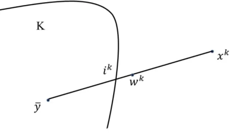
Lemma 3.10. Letxk_{be an iterate for Algorithm 3.1. LetL}k_{be the line segment connectingx}k_and

¯

y, andikbe the point of intersection ofK andLk. If we use binary search onLkto find a pointwk

on it such thatwk∈/ K, then we have

kxk_−wk_k

2

kxk_−ik_k

2

≥ 1

2. (3.19)

Figure 3.3:wkis closer toikthanxk

The binary search will generate a finite sequenceu1, u2, ..., ur(=wk)withwk = ur−1₂+xk. Since the search terminates atur,ur−1∈K. That is,

kxk−ur−1k₂ ≥ kxk−ikk₂.

Thereforekxk _−wk_k

2 ≥ kxk−w0k2, wherew0 = (x

k_+ik₎

2 is the mid point of the line segment

joiningxk_andik_{. That is,}

kxk_−wk_k

2

kxk_−ik_k

2

≥ kx

k_−w0_k

2

kx−ik_k

2

≥ 1 2.

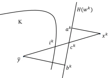
connectingxkandy¯, andK. The following figure illustrates the situation.

Figure 3.4:dist(xk, K)is related to thatdist(xk, H−(wk))

We will drop the super-scripts for the sake of brevity. Since the trianglesbyc¯ andaxcare similar, we have

ka−xk2 =

kx−ck2ky¯−bk2

ky¯−ck₂ . (3.21)

Letd=dist(¯y, bd(K)). Clearlyky¯−bk2 ≥d >0. Note that since the sequence{xk}is bounded

(Lemma 3.9), so is the sequence{y¯−ck_{}. So there exists anN >0such thatky¯−c}k_k

2 ≤N for

allk. Hence,

ka−xk₂ ≥ d

Nkx−ck2. (3.22)

Sincex /∈K, the hyperplaneH−(x)separatesxfromKstrictly. Hence

kx−ck₂ ≥ kx−wk₂.

From Lemma 3.10, we have

kx−wk2 ≥

1

2kx−ik2.

Hence

kx−ck₂≥ 1

Alsokx−ik₂ ≥dist(x, K). These inequalities, together with (3.22), imply

dist(xk, H−(wk)) =ka−xk2 ≥

d

2Ndist(x, K), (3.23)

which is the same as (3.28) withδ = ₂d_N. N can be made larger to makeδ <1.

For the general case, whenG 6=I, we use the equivalence of norms and (3.23) for the proof. It is known that

M1kxkG≤ kxk2 ≤M2kxkG, (3.24)

for some constantsM1andM2. So we have

distG(x, H−(w)) =kx−ΠH−_(w),G(x)k_G≥

kx−ΠH−_(w),G(x)k₂

M2

.

Since

kx−Π_H−_(w),G(x)k₂≥ kx−Π_H−_(w)(x)k₂=dist(x, H−(w)),

we have

distG(x, H−(w))≥

dist(x, H−(w)) M2

. (3.25)

Using a similar argument, we observe that

dist(x, K) =kx−ΠK(x)k2 ≥M1kx−ΠK(x)kG≥M1kx−ΠK,G(x)kG. (3.26)

From (3.23), (3.25), and (3.26), we get

distG(x, H−(w))≥

d 2N

M1

M2

Proof. Letuk= Π_H−_(wk_),G(xk). By (3.11) of Lemma 3.7

distG(uk, K)2 ≤distG(xk, K)2− kuk−xkk2G. (3.29)

From Lemma 3.11, we have aδ >0such that

distG(xk, K)×δ≤distG(xk, H−(wk))∀k. (3.30)

Since0< δ≤1, we have

distG(xk, K)2× −δ2 ≥ −distG(xk, H−(wk))2 ∀k. (3.31)

Note thatdistG(xk, H−(wk)) =kuk−xkkG. From (3.31) and (3.29), we get

distG(uk, K)2 ≤ distG(xk, K)2+distG(xk, K)2× −δ2

= (1−δ2)distG(xk, K)2 (3.32)

which is the same as (3.28) withµ=√1−δ2_.

Lemma 3.13. For any sequence{xk_{}generated by Algorithm 3.1, we have}

lim

k→∞dist(x

k_{, K) = 0.}

Proof. The arguments in this proof are similar to the proof of Lemma 15 of (Censor and Gibali, 2008).

IfF(xk) = 0, thenxk+1 = Π_H−_(wk_),G(xk). Hence from Proposition 3.12, we have

distG(xk+1, K)≤µ×distG(xk, K). (3.33)

Otherwise, from (3.29), we get

Also, there exists aµ∈[0,1)such that

distG(ΠH(_wk_),G(xk), K)≤µ×distG(xk, K). (3.35)

From the non expansiveness of projector, we get

kxk+1−Π_H−_(wk₎(xk)k2_G = kΠ_H−_(wk_),G(pk)−Π_H−_(wk₎(xk)k2_G

≤ kpk−xkk2_G

≤ kxk_−ρ kG−1

F(xk) kF(xk_)k

2

−xkk2

G

≤ kρ_kG−1 F(x

k₎

kF(xk_)k

2

k2_G

≤ ρ2_kν−1,

whereνis the smallest eigenvalue ofG. That is

kxk+1−Π_H−_(wk₎(xk)k_G≤

ρk

√

ν. (3.36)

By triangle inequality withGnorms, we get

kxk+1_−Π

K,G(ΠH−_(wk₎(xk))k_G

=kxk+1_−Π

H−_(wk₎(xk) + Π_H−_(wk₎(xk)−Π_K,G(Π_H−_(wk₎(xk))k_G

≤ kxk+1_−Π

H−_(wk₎(xk)k_G+kΠ_H−_(wk₎(xk)−Π_K,G(Π_H−_(wk₎(xk))k_G.

SinceΠK,G(ΠH−_(wk₎(xk))∈K,

where the last inequality follows from Proposition 3.12. The result follows from Lemma 3.8.

Lemma 3.14. For any sequence{xk_{}generated by Algorithm 3.1, we have}

lim

k→kx

k+1_−xk_k G = 0.

Proof. The arguments in this proof is similar to the proof of Lemma 16 of (Censor and Gibali, 2008).

IfF(xk) = 0,

kxk+1−xkkG = kΠH−_(wk_),G(xk)−xkkG

= distG(xk, H−(wk))

≤ distG(xk, K). (3.38)

If there is a subsequence{xr_{}, withr ∈ R ⊂ {1,2, ...}, of{x}

k}withF(xr) = 0, then from the above inequality and the previous Lemma, we getkxr+1_−xr_k

G →0. IfF(xk)6= 0,

kxk+1_−xk_k

G = kxk+1−ΠH−_(wk_),G(xk) + Π_H−_(wk_),G(xk)−xkk_G

= kxk+1−Π_H−_(wk_),G(xk)k_G+kΠ_H−_(wk_),G(xk)−xkk_G

≤ √ρk

ν +distG(x

k_{, H}−_(wk₎₎

≤ √ρk

ν +distG(x

k_{, K) (3.39)}

where the last inequality follows from the fact thatH−(wk)⊂K. Since bothdistG(xk, K)andρk go to zero, the proof is complete.

Theorem 3.15. The sequence generated by Algorithm 3.1 converges to a solutionx∗of VI(K, F).

Proof. The proof is same as that in (Censor and Gibali, 2008) and (Fukushima, 1986).

variables, mis the number of constraints, and1nrefers to the vector in Rn with all components

equal to1.

Example 3.1. n= 3, m= 1,

F(x) =x−1,

K ={x∈R3|

3

X

i=1

x2_i ≤1},

x0 = 0×1n,

Solution= 0.5774×1n.

Example 3.2. n= 5, m= 1,

F(x) =x−1,

K ={x∈_R5_| 5

X

i=1

x2_i ≤2},

x0 = 0×1n,

Solution= 0.6325×1n.

Example 3.3. n= 10, m= 1,

F(x) =x−1,

K ={x∈_R10_| 10

X

i=1

x2_i ≤5},

x0 = 0×1n,

Solution= 0.7071×1n.

Example 3.4. n= 20, m= 1,

F(x) =x−1,

K ={x∈R20|

20

X

i=1

x2_i ≤15},

x0 = 0×1n,

Example 3.6. n= 3, m= 1,

Fi(x) =x3_i −1,

K ={x∈_R3_| 3

X

i=1

x2_i ≤1},

x0 = 0×1n,

Solution= 0.8660×1n.

Example 3.7. n= 3, m= 1,

F(x) =      

x1+ 0.2x31−0.5x2+ 0.1x3−4

−0.5x1+x2+ 0.1x32+ 0.5

0.5x1−0.2x2+ 2x3−0.5

      ,

K ={x∈R3|x21+ 0.4x22+ 0.6x23 ≤1},

x0 = [0,1,1],

Solution= [1,0,0].

Table 3.1: Comparison of FRPM vs IAPRPM Example FRPM iterations IAPRPM iterations

1 7 3

2 6 3

3 5 3

4 5 4

5 7 3

6 7 3

7 9 10

3.2

A gap function based algorithm

Both the IAPRPM and FRPM algorithms require Assumtion F3 to hold. Although these al-gorithms are easy to implement, the assumption may not hold for general variational inequality problems. To that end, the first part of this section analyses a gap function which can be evaluated using either of the two RPMs.

3.2.1 The gap function

Let us recall the generic gap function from Zhu and Marcotte’s framework (Zhu and Marcotte, 1994). LetΩ(y, x) :K×K→_Rbe non-negative, continuously differentiable onK×K, strongly convex onKwith respect toyfor allx∈Kand satisfy

Ω(x, x) = 0andOyΩ(x, x) = 0 ∀x∈K. (3.40)

Define

h(y, x) =hF(x), x−yi −Ω(y, x), (3.41)

g(x) = max

y∈Kh(y, x) =h(H(x), x), (3.42) whereH(x)is the unique maximizer of h(y, x)overK. Since the problem of findingg(x)is to maximize a strongly convex objective function over a convex set,H(x)is unique.

In this section, we assume K is a compact, convex set. Note that the variables in most ap-plications have some natural upper and lower bounds, so it is not too restrictive to make such an assumption. Consider the following choice ofΩ :K×K →R,

Ω(u, v) = 1

2(u−v)

then theAV I (2.20) can be solved by any of the relaxed projection methods, see Proposition 3.17 and the comments following it.

Proposition 3.16. For a positive definite matrixG,

Ω(y, x) =hy−x, G(y−x)i

satisfies (3.40). Proof. Note that

OyΩ(y, x) = 2G(y−x)

and

OxΩ(y, x) = 2G(x−y).

Hence

hOyΩ(y, x) +OxΩ(y, x), y−xi= 0.

WithΩ(y, x) =Mhy−x, y−xi, theAV I(x)takes the following form

hF(x) + 2M(y−x), w−yi ≥0 ∀w∈K. (3.44)

LetS(y) =F(x) + 2M(y−x). For a fixedx∈K,S(y)is the function that defines the AVI (3.44). Proposition 3.17. S(y) satisfies (3.13) with z = 0 and D as the closed ball of radius r = max{1,2kxk2}around the origin.

Proof. Considery∈_Rn_{such thatkyk}

2>max{1,2kxk2}. We have

hS(y), yi = hF(x) + 2M(y−x), yi

= hF(x), yi+Mkyk₂2+Mkyk2₂−2Mhx, yi

by the definition ofM. Sincekyk₂ >1,−kyk₂ ≥ −kyk2

2. Also note that the factkxk2 ≤ kyk2/2

implies that last two terms in the above inequality add to a non-negative number. Hence, we have

hS(y), yi ≥ kyk2₂ ≥ kyk2. (3.45)

Since the only variable term inS(y)is2M y,α= 1satisfies (3.13) for the AVI.

Proposition 3.17 shows that we can use the relaxed projection method to solve theAV I(xk). Note that the defining functionS(y) =F(x) + 2M(y−x), forAV I(x), is zero at

O(x) =x−F(x) 2M .

SinceM >max

x∈KkF(x)k,O(x)usually is close tox. Ifc(O)≤0, thenO(x)∈K and no iterative procedure is required to solve AVI(x), andH(x) = O(x). In this case, the value ofg(x) can be found as,

g(x) = hF(x), x−O(x)i −MhO(x)−x, O(x)−xi

= hF(x),−F(x)

2M i −Mh F(x)

2M , F(x)

2M i

= kF(x)k

2 2

4M . (3.46)

Ifx1 andx2are two points such thatx2=H(x1) =O(x1)andO(x2)∈K, then we have

g(x1) = kF(x

1_)k2 2

4M (3.47)

g(x2) = kF(x

2_)k2 2

4M

= kF(x

1₋F(x1₎

2M )k22

for someλ <1providedO(x1)andO(x2)are feasible. With the given choice ofΩ, the following algorithm, which is a modification of the Zhu and Marcotte’s general framework can be proved to converge to a solution of VI(K, F).

3.2.2 The algorithm

Algorithm 3.2Descent algorithm

Initialization: Selectx0 ∈K,γ, β, σ∈(0,1). Setk= 1, loop= 0. whileloop = 0do

ifxk∈SOL(K, F)then Set loop = 1.

else

ifO(xk) =xk− F₂(_Mxk) ∈Kthen Setxk+1_=O(xk_).

else

Solve AVI(xk) forH(xk).Definedk=H(xk)−xk. ifg(xk+dk)< γg(xk)then

Setxk+1 =xk+dk =H(xk). else

Select the smallest integermsuch that

g(xk)−g(xk+βmdk)≥ −σβm_hOg(xk_{), d}k_i,

and setxk+1 =xk+βmdk. end if

end if

Setk=k+ 1.

we have

g(xk+1)≤λg(xk)

for someλ∈ (0,1). If there are an infinite number of such finite subsequences, we can combine them to get an infinite sub sequence of iterates for which the gap function value converges to zero.

Rest of the proof is the same as that of Theorem 6.1 in (Zhu and Marcotte, 1994).

I have conducted tests on two small examples to check the effectiveness of this algorithm. I used the RPM of (Fukushima, 1986) to solve the AVIs. The numerical experiments showed a shortcoming in Fukushima’s algorithm. It does not converge in practice if the solution to the VI(K,

F) is not at the boundary ofK. That is, whenF(x∗) = 0. The problem is possibly due to the fact that division bykFk, which can be a very small number in the neighborhood of a zero ofF, may cause inaccuracy in the computation. The IAPRPM overcomes this hurdle by first checking if an iterate is a zero ofF.

If the zero ofS(y) is not feasible, we can start with the origin as the initial guess for solving

AV I(xk)with either of the RPMs. We can also start withx0 = 0as the first iterate for Algorithm 3.2. If the initial guess is not close to the boundary of setK, the iterates moves quickly towards the boundary, without the need for solving theAV I(xk)with fukushima’s method since the zero of

S(y), being close to the current iterate, is feasible for the first few iterations. I conducted the numerical tests on the following two examples.

Example 3.8. This example is used for testing the RPM in (Fukushima, 1986).

F =



    

2x1+ 0.2x31−0.5x2+ 0.1x3−4

−0.5x1+x2+ 0.1x32+ 0.5

0.5x1−0.2x2+ 2x3−0.5



    

Example 3.9. I created this simple two dimenional example for testing.

F =



 

3x1+x2−5

2x1+ 5x2−3



 

K = {x∈R2|x21+x22 ≤1}.

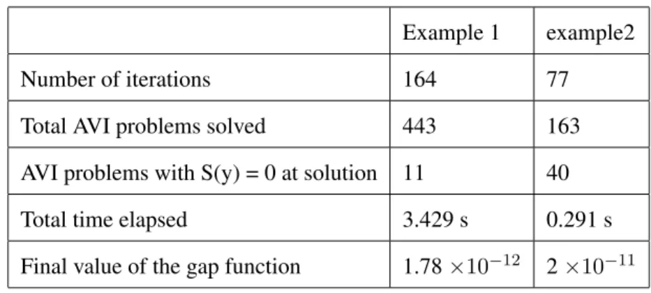
The solutions to these problems are(1,0,0)and(0.9890,0.1480)respectively. I used the same parameters for both the problems:β = 0.7, σ= 0.5, γ= 0.9, M = 20. The stopping criteria used iskxk_−xk+1_{k ≤0.00001. The following table summarizes the test results.}

Table 3.2: Results for the descent algorithm

Example 1 example2

Number of iterations 164 77

Total AVI problems solved 443 163

AVI problems with S(y) = 0 at solution 11 40

Total time elapsed 3.429 s 0.291 s

Final value of the gap function 1.78×10−12 2×10−11

As the table shows, in both the examples no iterative procedure was required to solve the AVIs for first few iterations. The total number of AVIs solved is significantly more than the number of iterations since the g(xk+dk) < γg(xk) condition of Algorithm 3.1 does not hold for many iterations.