& October 1, 2019
The polarimetric imaging mode of VLT/SPHERE/IRDIS I:
Description, data reduction and observing strategy
?J. de Boer
1, M. Langlois
2,3, R. G. van Holstein
1,4, J. H. Girard
5, D. Mouillet
6, A. Vigan
3, K. Dohlen
3, F. Snik
1,
C. U. Keller
1, C. Ginski
1,7, D. M. Stam
8, J. Milli
4, Z. Wahhaj
4, M. Kasper
9, H. M. Schmid
10, P. Rabou
6, L. Gluck
6,
E. Hugot
3, D. Perret
11, P. Martinez
12, L. Weber
13, J. Pragt
14, J.-F. Sauvage
15, A. Boccaletti
11, H. Le Coroller
3,
C. Dominik
7, T. Henning
16, E. Lagadec
12, F. Ménard
6, M. Turatto
17, S. Udry
13, G. Chauvin
6, M. Feldt
16, and
J.-L. Beuzit
3(Affiliations can be found after the references)
Received October 1, 2019; Accepted TBD
ABSTRACT
Context.Polarimetric imaging is one of the most effective techniques for high-contrast imaging and characterization of protoplane-tary disks, and has the potential to become instrumental in the characterization of exoplanets. The Spectro-Polarimetric High-contrast Exoplanet REsearch (SPHERE) instrument installed on the Very Large Telescope contains the InfraRed Dual-band Imager and Spec-trograph (IRDIS) with a dual-beam polarimetric imaging (DPI) mode, which offers the capability to obtain linear polarization images at high contrast and resolution.
Aims.We aim to provide an overview of the polarimetric imaging mode of VLT/SPHERE/IRDIS and study its optical design to improve observing strategies and data reduction.
Methods.ForH-band observations of TW Hydrae, we compare two data reduction methods that correct for instrumental polarization effects in different ways: a minimization of the ’noise’ image (Uφ), and a polarimetric-model-based correction method that we have developed, as presented in Paper II of this study.
Results.We use observations of TW Hydrae to illustrate the data reduction. In the images of the protoplanetary disk around this star we detect variability in the polarized intensity and angle of linear polarization with pointing-dependent instrument configuration. We explain these variations as instrumental polarization effects and correct for these effects using our model-based correction method.
Conclusions.The polarimetric imaging mode of IRDIS has proven to be a very successful and productive high-contrast polarimetric imaging system. However, the instrument performance is strongly dependent on the specific instrument configuration. We suggest adjustments to future observing strategies to optimize polarimetric efficiency in field tracking mode by avoiding unfavourable dero-tator angles. We recommend reducing on-sky data with the pipeline called IRDAP that includes the model-based correction method (described in Paper II) to optimally account for the remaining telescope and instrumental polarization effects and to retrieve the true polarization state of the incident light.
Key words. Polarization - Techniques: polarimetric - Techniques: high angular resolution - Techniques: image processing - Proto-planetary disks
1. Introduction
1.1. High-contrast and resolution imaging polarimetry
Imaging planets and protoplanetary disks in the visible and near-infrared (NIR) requires the observer to account for the large contrasts between bright stars and their faint surroundings. Po-larimetry has proven to be a powerful tool for high-contrast imaging, e.g. with HST/NICMOS (Perrin et al. 2009), Sub-aru/HiCIAO (Mayama et al. 2012) and VLT/NACO (Quanz et al. 2011). When starlight is scattered by circumstellar material it be-comes polarized. Therefore it is possible to distinguish this scat-tered light from the predominantly unpolarized stellar speckle halo by computing the difference between two images recorded in two orthogonal polarization states. This high-contrast imaging technique is known as Polarimetric Differential Imaging (PDI;
Kuhn et al. 2001). With the aid of adaptive optics (AO),
po-? Based on observations made with ESO Telescopes at the La Silla
Paranal Observatory under programme ID 095.C-0273(D)
larimetric imaging has been succesful in detecting faint circum-stellar disks down to very small separations (∼0.100; e.g.Quanz
et al. 2013;Garufi et al. 2016). Compared to alternative
high-contrast imaging techniques such as Angular Differential Imag-ing (ADI;Marois et al. 2006), PDI is especially well suited to image disks seen close to face-on, such as TW Hydrae (seen∼7◦ from face-on orientation;Rapson et al. 2015;van Boekel et al. 2017). While ADI suffers from self-subtraction of signal from a disk with a low inclination, PDI remains sensitive to its scattered light. PDI will remove unpolarized stellar and disk signal alike, which makes this technique only less suitable to detect disks with very low degrees of polarization due to unfavorable scatter-ing angles (close to 0◦or 180◦) or grain sizes much larger than the wavelength (Hansen & Travis 1974). Fortunately, the scatter-ing surfaces of protoplanetary disks predominantly contain sub-micron sized grains (i.e. smaller than the typical wavelengths at which high-contrast imaging instruments operate), while the single-scattering angles in most regions of any circumstellar disk will not be close to 0◦or 180◦.
Apart from being an effective high-contrast imaging tech-nique, polarimetry offers the potential to characterize scattering particles in circumstellar disks and the atmospheres of exoplan-ets. Radiative-transfer modeling of disks is heavily plagued by degeneracies when the models are based on the Spectral Energy Distribution (SED) alone (e.g.Andrews et al. 2011;Dong et al.
2012).Perrin et al.(2015) andGinski et al.(2016) have used the
resolved polarimetric surface brightness to determine the scat-tering phase function for the debris disk around HR 4796A (see
alsoMilli et al. 2015) and HD 97048, respectively. The scattering
phase function will be instrumental in the unambiguous charac-terization of micron-sized dust particles.
Young self-luminous giant exoplanets or companion brown dwarfs can also be polarized at NIR wavelengths, as their ther-mal emission is scattered by cloud and haze particles in the companions’ outer atmospheres or dust particles surrounding the companions (Sengupta & Marley 2010; de Kok et al. 2011;
Marley & Sengupta 2011;Stolker et al. 2017). Substellar
com-panions are observed as point sources, and only produce a significant (integrated) polarization signal if the shapes of these companions projected on the image plane deviate from circu-lar symmetry. Measuring a pocircu-larization signal from a compan-ion confirms the presence of a scattering medium (e.g. clouds) and can trace the cloud morphology (e.g. horizontal bands), ro-tational flattening, the projected spin-axis orientation and the shape and orientation of a disk around the companion.
1.2. The polarimetric mode of the VLT/SPHERE INfraRed Dual-band Imager and Spectrograph: IRDIS/DPI
In 2014, the Spectro Polarimetric High-contrast Exoplanet RE-search (SPHERE; Beuzit et al. 2019) instrument was commis-sioned at Unit Telescope 3 (UT3) of the Very Large Telescope (VLT). This instrument contains the extreme-AO system SAXO (SPHERE AO for eXoplanet Observation; Fusco et al. 2006,
2016), that consists, among other components of a high-order deformable mirror (DM) with 41×41 actuators and a Shack-Hartmann wavefront sensor that can operate up to 1200 Hz
(Fusco et al. 2016). The wavefront sensor records in the
visi-ble regime and performs best for stars ofR=9−10 mag, where it typically yields a Strehl ratio of≥90%. Still, up to the magni-tude limit ofR=14−15 mag the AO system improves the perfor-mance with a factor of∼5 (Beuzit et al. 2019). This extreme-AO system supports three scientific subsystems: the (visible-light) Zurich IMaging POLarimeter (ZIMPOL; Schmid et al. 2018), the (NIR) Integral Field Spectrograph (IFS;Claudi et al. 2008), and the (Near) InfraRed Dual-band Imager and Spectrograph (IRDIS;Dohlen et al. 2008).
IRDIS is primarily designed to detect planets in differential imaging modes combined with pupil tracking, where the tele-scope pupil remains fixed on the detector and the image ro-tates with the parallactic angle. This rotation of the image dur-ing observations allows the removal of the stellar speckle halo by performing ADI. A beam splitter ensures that the star is im-aged twice on the detector. Wide-band, broad-band or narrow-band filters can be inserted in a common filter wheel upstream from the beamsplitter to allow what is called ’classical imaging’. Downstream from the beam splitter, another wheel is present with which we can introduce two different filters for the sepa-rate beams. Observations in two different color filters allows the detection of planets (e.g. by observing methane absorption in their atmosphere) with Dual-Band Imaging (DBI; e.g.,
Rosen-thal et al. 1996;Racine et al. 1999; Marois et al. 2000;Vigan
et al. 2010).
The inclusion of orthogonal linear polarization filters (po-larizers) in this second filter wheel makes IRDIS a polarime-ter. In this Dual-beam Polarimetric Imaging (hereafter DPI or IRDIS/DPI; Langlois et al. 2014) mode, a rotatable half-wave retarder is inserted in the common path of SPHERE to modulate between the linear polarization components. IRDIS/DPI is cur-rently offered in field and pupil tracking. The requirements for DBI contrast have provided high image quality from which also DPI benefits, in particular, high image stability that is essential for coronagraphy (Boccaletti et al. 2008;Carbillet et al. 2011;
Guerri et al. 2011), and most importantly a very low differential
wave-front error between the two beams (Dohlen et al. 2016). Since IRDIS/DPI was first offered to the community during the science verification of SPHERE in december 2014, it has proven to be a very succesful and productive mode for high-contrast imaging of circumstellar disks (e.g.,Benisty et al. 2015;Stolker
et al. 2016;Garufi et al. 2017;Avenhaus et al. 2018;Pinilla et al.
2018), but it also shows great promise for the characterization of polarized substellar companions.Van Holstein et al. (2017) have used IRDIS/DPI to search for a polarization signal in the companions around HR 8799 and PZ Tel, similar to the attempts made with GPI for HD 19467 B byJensen-Clem et al.(2016) and βPic b byMillar-Blanchaer et al.(2015). AlthoughVan Holstein
et al.do not detect a polarization signal for the companions of
either star, they do present stringent upper limits on the polariza-tion of∼0.1% for PZ Tel B, and∼1% for the much fainter planets around HR 8799. Furthermore they present a polarized contrast of∼10−7at 0.5" separation from the primary star HR 8799.
Due to the complexity of the SPHERE instrument and its many reflecting surfaces, the polarimetric performance is strongly dependent on the specific instrumental setup. Each opti-cal component in the telescope and instrument can cause
instru-mental polarization effects, which we group in two categories:
1) the introduction of polarization, and 2) the mixing of po-larization states in the light beam, which we callInstrumental
Polarization(hereafterIP, to avoid confusion with the
overar-ching term "instrumental polarization effects") and polarimetric
crosstalk, respectively.IPcan give the false impression of a
de-tection of polarization where there is in fact no true polarization signal incident on the telescope. Crosstalk can change incident polarization into a state that is not being measured by the instru-ment (e.g., linear to circular polarimetry, see Sect.2). Therefore, crosstalk can decrease thepolarimetric efficiency: the fraction of measured polarization over the incident polarization. Unlike the polarimetric mode of ZIMPOL, no hard requirements where defined for the polarimetric performance of IRDIS, because the initial science priority of this mode was determined to be low. Lower instrumental polarization effects were expected in the NIR than in the visible. Furthermore, because of the difficulty of the system analysis required to predict and correct these effects beforehand, the choice was made to rely on a-posteriori charac-terisation of the DPI mode, whenever possible.
will describe a correction method based on this model to ac-count for the instrumental polarization effects and compute the true polarization signal incident on the telescope. This correc-tion method is included in a new data-reduccorrec-tion pipeline called IRDIS Data reduction for Accurate Polarimetry (IRDAP), which we will make public (see Paper II).
Paper I begins with a general description of polarization and dual-beam polarimetric imaging in Sect.2. We will describe the optical components encountered by the light beam in Sect.3. In Sect.4, we will explain the basic principles behind the data reduction, which we will apply in Sect.5.1on the TW Hydrae observations of van Boekel et al. (2017). In the reduced data of TW Hydrae we detect an instrument-configuration-dependent variation in the polarization signal, which we will use to il-lustrate the polarimetric performance of IRDIS/DPI. In the re-mainder of Sect.5 we will describe the instrumental polariza-tion effects of SPHERE/IRDIS with the use of the polarimetric instrument model of Paper II. These instrumental polarization effects will enable us to explain the instrument-configuration-dependent variations in TW Hydrae. In Sect.6we will apply the correction method described in Paper II to account for the in-strumental polarization effects and obtain the true polarization state for TW Hydrae. We will compare the results of the IR-DAP reduction, (with the model-based correction method) with the results of the best ’conventional’ data reduction, where we apply an empirical correction method. Based on our analysis, we will propose recommendations for future observations and possible SPHERE upgrades to enhance the polarimetric perfor-mance in Sect.7. In Sect.8we will make a comparison between SPHERE/IRDIS/DPI and major contemporary AO-assisted po-larimetric imagers in the NIR. We will end Paper I with our con-clusions and recommendations in Sect.9.
2. Dual-beam Polarimetric Imaging
2.1. Polarization conventions and definitions
Elliptical polarization (partial and full) is conveniently described
byStokes(1851) with what is known as the Stokes vector:
S=
I Q U V
, (1)
where I is the total intensity of the beam of light; Q and U
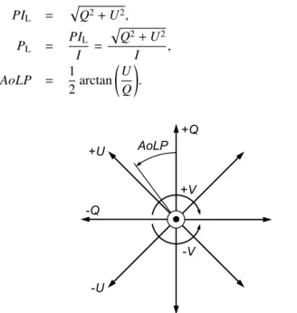
describe the two linear polarization contributions; and V de-scribes circular polarization. In the literature, the +Q direc-tion is often aligned with the local meridian (e.g.,Witzel et al. 2011). In Sect.4we have used this convention for+Q. Although this choice of reference frame is arbitrary, it is the convention adopted by the International Astronomical Union. As illustrated in Fig.1, we have used the following conventions for the re-maining orientations: For a beam propagating along thez-axis (in the direction of increasingz) in a right-handedx, y,z coordi-nate system, let+Qdescribe linear polarization with a prefered oscillation in the ±xdirection (which we align with our frame of reference, e.g., the meridian);−Qthen oscillates in the±y di-rection;+Udescribes linear polarization oscillating at an angle of+45◦from thex-axis (rotated in counter-clockwise direction
when looking at the source, and−45◦from they-axis); while−U
polarized light oscillates at an angle of−45◦(or+135◦) with
re-spect to thex-axis. When the observer is facing towards the−z
direction,+V describes circular polarization where the peak of
the electric field rotates clockwise (i.e. moving from+xto−y) and−Vdescribes counter-clockwise rotation.
IRDIS/DPI is designed to measure linear polarization only, which is expected to be the dominant polarization component caused by scattering at the surface layers of protoplanetary disks and substellar companions. From the Stokes vector components, we can determine the linearly Polarized Intensity (PIL); Degree
and Angle of Linear Polarization (DoLPorPL&AoLP,
respec-tively) according to:
PIL =
p
Q2+U2, (2)
PL =
PIL
I =
p
Q2+U2
I , (3)
AoLP = 1
2arctan
U Q
!
. (4)
+Q AoLP
+V -Q
+U
-U
-V
Fig. 1.Orientation of the Stokes vector components of Eq.1, where the
beam is propagating out of the paper towards the reader. After the verti-cal axis (+Q) is aligned with a prefered orientation (usually the meridian on-sky), the remaining Stokes vector components are oriented accord-ingly. The Angle of Linear Polarization (AoLP, Eq.4) is also measured with respect to the+Qdirection in counter-clockwise direction.
2.2. The polarimetric imager
Although ideal polarimeters do not exist, such a hypothetical in-strument is helpful when we describe the general principles of PDI. Apart from mirrors and lenses the main components of this ideal polarimeter are two (in case of dual-beam) analyzers and detectors (or detector halves). The analyzers can either be two separate polarizers (which require an aditional, preferably non-polarizing beamsplitter upstream) with orthogonal polarization (also called transmission) axes or a polarizing beamsplitter. Let us choose the polarization axis of one analyzer (A1) to be aligned with the+Qdirection, and the other analyzer (A2) to be aligned with−Q. We can retrieve (or ‘indirectly measure’) the first two components of Eq. 1 by adding and subtracting the measured intensity of both beams (IA1/A2) of light, respectively:
I = IA1+IA2, (5)
Q = IA1−IA2. (6)
We can rephrase Eqs.5and6to describe the transmission of the analyzers:
IA1 =
1
2(I+Q), (7)
IA2 =
1
where for an ideal polarimeter, I and Qwill be equal to their counterparts incident on the telescope (IinandQin, respectively).
To retrieveU, we will either need to rotate the analyzers by 45◦or introduce an optical component that can rotate the polar-ization direction with the same angle. A half-wave (λ/2) plate (HWP) retards light that is polarized in the direction orthogonal to its fast axis withλ/2 compared to light that is polarized in alignment with its fast axis. Therefore, a HWP upstream from the beam splitter can be used to rotate the measured polariza-tion angle by ∆AoLP by placing the fast axis of the HWP at an angle of ∆AoLP/2 with respect to the polarization axes of the analyzers (Appenzeller 1967). It is possible to retrieve U
by placing the HWP at an angle θHWP =22.5◦ with respect to
the polarization axis of A1, which changes Eqs. 7 and8 into:
IA1/A2=(I±U)/2, and Eq.6will yieldU, instead ofQ. We now
see why the Stokes vector notation is convenient: its components are easilly retrieved from the observables of an ideal polarimeter, which ‘measures’ a Stokes vector unaltered by the telescope and instrument (i.e.S=Sin, whereSinis the incident Stokes vector).
Real polarimeters are never ideal: instrumental polarization effects depend on the specific instrument configuration used dur-ing observations. For complex instruments, the major instrumen-tal polarization effect is typically the introduction ofIPcaused by the large number of reflections in the telescope and instru-ment. We can correct for anyIPcreated downstream of the HWP by recordingQfor two HWP angles:θHWP =0◦& 45◦(see e.g.
Tinbergen 1996;Witzel et al. 2011;Canovas et al. 2011). The
secondθHWPchanges the signs of the beam’s originalQ
compo-nent but leaves theIPcreated downstream from the HWP unal-tered. Therefore, for non-ideal polarimeters we change the no-tation of thesingle-differencecomputations described by Eq.6
to measure Q+ = Q+IPforθHWP = 0◦, and Q− = −Q+IP
for θHWP = 45◦. Similarly, we rename the single-sumtotal
in-tensities determined with Eq.5for θHWP = 0◦ & 45◦ asIQ+ & IQ−, respectively. We then apply thedouble-differencemethod
to obtain the linear Stokes parameters corrected for IPcreated downstream of the HWP and the corresponding total-intensity images with thedouble sum:
Q = 1
2 Q
+−Q−, (9)
IQ =
1
2 IQ++IQ−
, (10)
U = 1
2 U
+−U−, (11)
IU =
1
2(IU++IU−), (12)
whereU+ =U+IPandIU+ are measured withθHWP =22.5◦,
whileθHWP=67.5◦yieldsU−=−U+IPandIU−.
The double difference does not removeIPcaused by the tele-scope and instrument mirrors upstream from the HWP, nor does it remove the most important crosstalk contributions. Correct-ing for these instrumental polarization effects requires that we determine the polarimetric response function for the polarimet-ric imager, as we do in Sect.5.2.1for the polarimetric mode of VLT/SPHERE/IRDIS.
3. Design of the polarimetric mode IRDIS/DPI
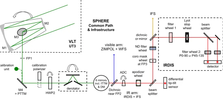
In this Section we describe the optical components of VLT/UT3, SPHERE’s Common Path and Infrastructure (CPI) and IRDIS that are most important because they either create instrumen-tal polarization effects, they are useful for calibrations or they
can be changed to modify the observational sequence or strat-egy. These optical components are illustrated in the schematic overview of the telescope and instrument in Fig.2. Especially reflections at high angles of incidence are highlighted because larger angles are more prone to introduce instrumental polariza-tion effects.
3.1. Telescope and SPHERE common path & infrastructure
SPHERE is installed on the Nasmyth platform of the alt-azimuth Unit Telescope 3. After the axi-symmetric (and therefore non-polarizing) reflections of the primary and secondary mirrors (M1 and M2), the third mirror (M3) of UT3 is used to direct the light towards the Nasmyth focus. M3 introduces the first reflection that breaks axi-symmetry with a 45◦angle of incidence.
Shortly after the beam enters SPHERE we reach Focal Plane 1 (FP1), where a calibration light source can be inserted. The first reflection in the light path within SPHERE is the pupil tip-tilt mirror (PTTM or M4, with a 45◦incidence angle), which
is the only mirror in SPHERE that is coated with aluminum.1 The remaining mirrors of SPHERE are all coated with protected silver for its higher reflectivity. A calibration polarizer with a fixed polarization angle can be inserted in the light path, just be-fore the beam encounters HWP2, the only HWP available for IRDIS/DPI. In field-tracking mode, HWP2 can be rotated for two reasons. The first reason is to switch between four angles (HWP switch anglesθsHWP=0◦,45◦,22.5◦and 67.5◦, where the superscript ’s’ is used to distinguish between switch angles and the true angle of HWP2) to measureQ±andU±with IRDIS. The second reason is to account for field rotation in order to keep the source polarization angle fixed relative to the analyzer for a given HWP2 switch angle in a polarimetric cycle. The next op-tical component downstream is the image derotator, composed of three mirrors that together form a ‘K’-shape (therefore also called K-mirror, with the subsequent angles of incidence of 55◦,
20◦and 55◦). The derotator rotates around the optical axis to sta-bilize either the field or the pupil on the detector. In AppendixA, we have included a detailed description of the tracking laws for HWP2 and the derotator in both field-stabilized and pupil-stabilized mode.
Multiple reflective surfaces with small angles of incidence follow in the AO common path, including the image tip-tilt mir-ror (ITTM), the 41×41 actuator high-order DM and three toric mirrors (Hugot et al. 2012). A dichroic beam splitter separates the light into a visible and a NIR arm just after Focal Plane 2 (FP2). Note that an additional focal plane exists between FP1 and FP2. However, we adopt the nomenclature commonly used in existing literature such as the SPHERE manual. The visi-ble light is reflected by the dichroic beam splitter and sent to SAXO’s wavefront sensor and when required also to ZIMPOL (currently not offered simultaneously with IRDIS or IFS). The NIR beam is transmitted by the dichroic beam splitter, and is then corrected for atmospheric dispersion, determined by the air-mass during the observations. Due to the low angles of incidence (≤2.17◦) on the prisms of the Atmospheric Dispersion Corrector
1 This coating gives M4 similar reflective properties as M3 of UT3,
IRDIS filter
wheel 1 splitter beam
HWP2
visible arm: ZIMPOL + WFS
IFS
IR arm:
IRDIS + IFS coro mask
wheel at FP3 dichroic or mirror
detector
derotator calibration
polarizer
VLT UT3
M4 = PTTM M3
M1
M2 SPHERE
Common Path & Infrastructure
calibration unit
Lyot stop wheel
ADC apodizer
wheel
differential tip-tilt sensor beam
splitter
filter wheel 2: P0-90 or P45-135
Dichroic near FP2 6 mirrors incl. ITTM & DM FP1
ND filter wheel
Fig. 2. Schematic overview of the telescope and SPHERE/IRDIS, showing the optical components that are relevant for the polarimetric imaging
mode. The curved arrows indicate components that rotate during an observation block. Reflections at angles of incidence≥45◦
in the instrument are represented with similarly large incidence reflections in the figure. The green beam shows the starlight before color filters are applied, blue represents visible light, red and orange represent NIR light (with the orange beam towards the IFS showing the shorter wavelengths).
(ADC), it is assumed not to cause significant instrumental polar-ization effects. The validity of this assumption is left for future investigation. The beam then goes through the apodizer wheel (which allows apodization of the pupil in combination with Lyot coronagraphs) and is sent to a beamsplitter, which transmits 2% of the H band to a differential tip-tilt sensor (DTTS) and reflects the remaining light at 45◦angle of incidence. The (main)
reflected beam then encounters the wheel containing NIR coro-nagraph (focal) masks (Boccaletti et al. 2008; Martinez et al. 2009) in FP3, and the Neutral Density (ND) filter wheel before reaching the final 45◦angle reflection that directs the beam
to-wards IRDIS. For this reflection a dichroic beam splitter is se-lected when we use IRDIS in concert with IFS. For modes that only use IRDIS, which is currently the case for polarimetry, a mirror is selected instead.
3.2. SPHERE/IRDIS
IRDIS is described in detail byDohlen et al.(2008). In this sub-section and in Fig.2, we summarize the optical components for a better understanding of the polarimetric performance of the sys-tem and for reference later in this paper. The optical components of IRDIS are located within a cryostat cooled to 100 K to reduce thermal background emission. The first optical component in-side IRDIS is a common filter wheel (FW1). The filters of FW1 are the only color filters that we can insert for the polarimetic mode, since FW2 contains the analyzer/polarizer pair. Besides narrow-band and spectroscopy filters, FW1 contains four broad-band filters which are offered for DPI (see Table1).
Next, the beam encounters a Lyot stop wheel that also in-cludes a mask for the pupil obscuration by M2 and its support structure (the "spider"). Directly downstream from the Lyot stop wheel, the beam is split by the non-polarizing beam splitter plate (NBS). The beam transmitted by the NBS is reflected by an
ex-Table 1. Central wavelength (λc), bandwidth (∆λ) and pixel scale
for SPHERE/IRDIS broad-band filters available in filter wheel 1. The wavelength and bandwidth are described on theESO website, the pixel scales come fromMaire et al.(2016,2018). The broad-band filters are listed here as BB_X, similar to ESO Observing Blocks (OBs), but they are frequently listed as B_X (on the ESO website and in the head-ers of FITS files under keyword INS1.FILT.NAME), and asX band in the main text.a)The pixel scale for BB_Y has not been calibrated.
Therefore, the value for theY2 filter fromMaire et al.(2016) has been adopted.
Filter λc(nm) ∆λ(nm) Pixel scale (mas/pix)
BB_Y 1043 140 12.283a ±0.009
BB_J 1245 240 12.263 ±0.009
BB_H 1625 290 12.251 ±0.009
BB_Ks 2182 300 12.265 ±0.009
tra mirror in the direction parallel with the beam reflected by the NBS (and therefore with the same angle of incidence as the reflected beam: 45◦). The beams are finally reflected by two identical spherical camera mirrors, which focus the beams on the detector (not shown in Fig.2).
3.3. Wire-grid polarizer pairs and beam splitter
The P0-90 analyzer set in FW2 filters the light with polarization angles perpendicular to and aligned with the plane of the Nas-myth platform: the plane in which all reflections downstream from the derotator occur. The P45-135 set polarizes at angles of 45◦and 135◦with respect to this plane. Measurements recorded
with P45-135 are highly sensitive to crosstalk introduced by all reflections in this plane. Therefore, we limit the study in Pa-pers I & II to the use of the P0-90 analyzer pair, while using HWP2 to switch betweenQ± andU± measurements, which is the default setup for DPI.
The polarizing beam splitter is not perfectly non-polarizing, which is corrected for when we use the double difference. Therefore we can use the first-order approximation that it does not introduce new polarization to the beam. Astro-physical objects in the field of high-contrast imaging typically have a very low degree of polarization when integrating the total beam, since this beam is dominated by the central predominantly unpolarized star. The polarizers will only transmit one polariza-tion state each, which means that both beams will loose∼50% of their photons.
4. Polarimetric data reduction
In this Section, we describe the basic steps of the polarimetric data reduction for the IRDIS/DPI mode. In Sect.5we will apply this to the data of TW Hydrae as published byvan Boekel et al.
(2017), and use the results to analyse the polarimetric perfor-mance of the system. Because these observations were recorded before we had performed polarimetric calibrations, we encoun-tered unexpected instrumental polarization effects that depend on the specific instrument configuration, and vary during the ob-serving sequence. We will describe and explain these effects in detail based on the polarimetric instrument model of Paper II. In Sect.6we compare the reduction of this data after a data-driven correction for instrumental polarization effects with a data re-duction after a correction based on the polarimetric instrument model.
To promote general understanding of the underlying princi-ples of the polarimetric data reduction and because our analy-sis of the data in the subsequent sections required non-standard tests, we did not use the official Data Reduction and Handling (DRH,Pavlov et al. 2008) pipeline but our own custom data re-duction routines described below. However, the pre-processing (background subtraction, flat fielding and centering) is very sim-ilar to what is done by DRH and therefore described in Ap-pendixB.
4.1. Post processing: polarimetric differential imaging
The single-difference images (Q+,Q−,U+, andU−) are
deter-mined frame by frame for the HWP angles: θHWPs = 0◦, 45◦, 22.5◦, and 67.5◦, respectively. The single-difference images
ob-tained from the four frames of each file (per HWP angle) are median combined. Q and U are computed with the double-difference method of Eqs. 9 and11, for each polarimetric cy-cle (also called ‘HWP cycy-cles’, containing the four switch angles of HWP2:θs
HWP = 0
◦, 45◦, 22.5◦, and 67.5◦). Accordingly, per
HWP angle the corresponding single-sum total-intensity images are created with Eq.5. With these single-sum images, we create per HWP cycle the double-sum total-intensityIQandIUimages
with Eqs.10and12, respectively.
A residual of the read-out columns (see feature c in Fig.B.1) remains visible in the double-difference images. Similar to how
Avenhaus et al. (2014) removed noise across detector rows
from NACO images, we remove these artifacts from the double-difference images by taking the median over the top and bottom 20 pixels (to avoid including signal from the star) on the im-age per individual pixel column (not the 64 pixel wide read-out column), and subtract this median value from the entire pixel column.
We perform a first-order correction forIPcreated upstream from HWP2 (i.e. by the telescope and M4) on theQandU im-ages of each polarimetric cycle. This correction method (as de-scribed byCanovas et al. 2011) is based on the assumption that the direct stellar light is unpolarized. We take the median of the
Q/Isignal over an annulus centered around the star (excluding the coronagraph mask) to obtain the scalarcQ(likewise, we
de-terminecU withU/I), multiply this scalar withI, and subtract
this from the Qimage. Hence, the IP-subtracted linear stokes components are:
QIPS = Q−IQ·cQ, (13)
UIPS = U−IU·cU. (14)
The size and location of the annulus over which to measurecQ
andcU can be adjusted to suit a particular dataset. Ideally, the
annulus should lie in a region that should only contain non-scattered starlight, with high signal in the IQ and IU images.
Therefore, the size and location of the annulus depends on the brightness of the central star and the size and shape of the cir-cumstellar material that has been observed.
We now use the possible user-specific derotator offset angle that can be found from the FITS header keyword INS4.DROT2.POSANG, together with the true north correction
of−1.7◦(Maire et al. 2018) to apply a software derotation in
or-der to align allIQ/U andQ/UIPS with north up and east left on
the detector.
4.2. Azimuthal Stokes parameters
To create the final polarization image we have two choices. In the first, most straight-forward method we compute the polar-ized intensity PIL according to Eq.2 for each HWP cycle and
median combine these to create a final (less noisy)PIL image.
The problem with this method is that the squares taken in Eq.2
boost the noise in each image. For example, artifacts seen as a bright positive or negative feature detected at a point in theQIPS
image where the signal should be∼0, (on the diagonal ‘null’ lines separating the positive from the negative signal in theQIPS
images) or a strong positive signal in a region whereQIPSought
to be negative, will be indistinguishable from true disk signal in thePIL image. This is actually a general problem we encounter
when computing PIL, but even more so when we are dealing
with images of short integration times, such as resulting from individual HWP cycles.
In stead, we have used a second option to combine the HWP cycles and create the cleanest image by computing the azimuthal Stokes parameters (Schmid et al. 2006):
Qφ = −QIPScos (2φ)−UIPSsin (2φ), (15)
Uφ = +QIPSsin (2φ)−UIPScos (2φ), (16)
whereφdescribes the azimuth angle, which can be computed for each pixel (orx, ycoordinate) as
φ=arctan xstar−x y−ystar
!
I
measIncreasing time / parallactic angle
Q
measU
measθ
der= 172.6°
θ
der= 166.5°
θ
der= 160.0°
θ
der= 154.8°
IPS IPS
Counts Counts Counts
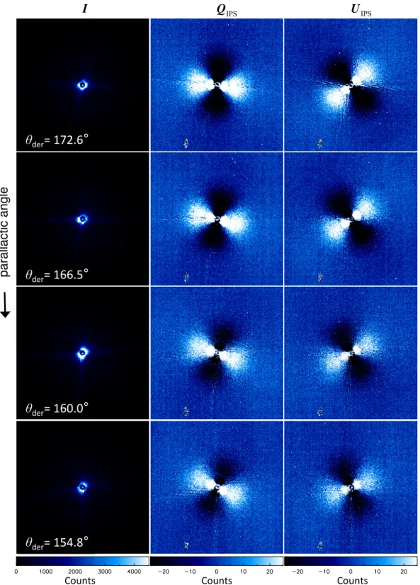
Fig. 3. Each row shows the I,QIPSandUIPS images (from left to right) for polarimetric cycles with increasing parallactic angle from top to
bottom. The on-sky orientation is the same for all panels: north is up, east is left. However, the measured polarization angle (Eq.4) is changing with derotator angle (θder), which we can see with the rotation of the butterfly pattern in clockwise direction. Furthermore, the polarimetric efficiency decreases withθderfurther removed from 180◦
, as we can see by the decreasing signal-to-noise ratio in theQIPSandUIPSimages.
The xandy positions of the central star in the image are de-scribed byxstarandystar, respectively. We can useφ0to give the
azimuth angle an offset if the measured polarization angle is not aligned azimuthally.φ0 is therefore referred to as the
polariza-tion angle offset.
Contrary to Eqs.15and16,Schmid et al.(2006) use the no-tationQrandUr, which have flipped signs compared toQφand
Uφ, respectively.Schmid et al.have chosen their conventions to
describe scattered light observations of the planets Uranus and Neptune, which is oriented in radial direction relative to the cen-ter of the planet. However, in protoplanery disks, we expect scat-tered light to produce predominantly azimuthally oriented polar-ization, which has motivated our choice of signs in Eqs.15and
polariza-tion angles oriented at±45◦with respect to azimuthal will result in±Uφsignal. Disks that have a high inclination or where mul-tiple scattering is expected to produce a significant part of the scattered light can contain a significant signal inUφ (Canovas
et al. 2015). However, for low-inclination disks we can expect all
scattering polarization to be in azimuthal direction. This means that Qφwill de facto show us PIL, with the benefit that we do
not square the noise, resulting in cleaner images. TheUφimage should ideally show no signal at all in this case, which makes it a suitable metric for the quality of our reduction.
5. Instrument-configuration dependence in polarimetric efficiency and polarization angle
5.1. Polarimetric observations of TW Hydrae
We have observed TW Hydrae during the night of March 31, 2015, with IRDIS/DPI. This data was recorded before we be-came aware of the most severe instrumental polarization effects for SPHERE/IRDIS. Therefore, these data have been recorded without taking recommendations (Sect.7) into account that op-timize the polarimetric efficiency of DPI observations. Further-more, the near face-on orientation of this disk (inclination=7◦,
Qi et al. 2008), allows us to assume azimuthal polarization after
scattering, which makes this object an ideal test case to illustrate how instrumental polarization effects alter the incident polarized signal.
The data have been recorded inHband (see Table1), using field-stabilized mode, while an apodized pupil Lyot coronagraph
(Carbillet et al. 2011;Guerri et al. 2011) with a focal plane mask
with radius of 93 mas was used. We have performed the obser-vations using a detector integration time (DIT) of 16 s per frame, four frames per file, during 25 polarimetric cycles. This adds up to a total exposure time of 106.7 min.
After creating the double-difference images we removed five HWP cycles with bad seeing and/or AO corrections. Therefore, the final dataset we have used for this analysis contains 20 sets ofQ,U,IQandIUimages.
Figure3shows theI = (IQ+IU)/2, QIPSandUIPS images
for four polarimetric cycles observed with increasing parallac-tic angle for each subsequent panel row. While each QIPS and
UIPS panel displays the typical ‘butterfly’ signal of an
approxi-mately face-on and axi-symmetric disk, strong variations occur between the polarimetric cycles: the butterflies appear to rotate in clockwise direction and the signal in theQIPSandUIPSimages
decreases with increasing parallactic angle. Since the observa-tions were taken in field tracking mode, the image of the disk itself does not rotate on the detector, rather the AoLP (Eq.4) is changing between the polarimetric cycles. We do not expect either the incident (‘true’) Degree or Angle of Linear Polariza-tion to vary with parallactic angle. Notice thatIremains roughly constant in Fig.3, thus a decrease in measuredPIL can only be
explained by a decrease inPL. Therefore, the changes inPLand
AoLPmust be caused by instrumental polarization effects that depend on the specific telescope and instrument configuration, which varies with the parallactic and altitude angle of the ob-served star.
5.2. Instrumental polarization effects
The calibrations of instrumental polarization effects and the analysis towards a complete Mueller matrix model of the instru-ment are described in detail in Paper II. In this section we will
briefly summarize how we have derived the model from calibra-tion measurements, and describe the instrumental polarizacalibra-tion effect of eachset of optical components. Here we consider opti-cal components to form a ‘set’ when they share a fixed reference frame, i.e. a common rotation of the set of components. For the last set of components (CPI+IRDIS components downstream of the derotator) we only fit the diattenuation, since crosstalk is absent because all reflections are aligned with the anlyzers.
In Sect.5.3we use this polarimetric instrument model to ex-plain variations detected in the degree and angle of linear po-larization in the data of TW Hydrae. Based on the polarimetric instrument model we have devised a correction method in Pa-per II. In Sect.6of this paper we apply this correction method to retrieve the true incident polarization for the observations of TW Hydrae.
5.2.1. From calibrations to polarimetric instrument model
In Paper II, we have used the internal light source with a cali-bration polarizer to create 100% polarized light, and measured the linear Stokes parameters for a wide range of instrumental configurations. We then defined the measured degree of linear polarization for the 100% polarized incident light to be equal to the polarimetric efficiency for this configuration. For each set of optical components including and downstream of the HWP, we have fitted the measured Stokes parameters to the wavelength-dependent retardance of this set of components. Similarly, we have calibrated the diattenuation of these sets of optical compo-nents with the internal light source, this time without the inclu-sion of a calibration polarizer to insert nearly unpolarized inci-dent light.
We have calibrated the diattenuation of the telescope and M4 (both located upstream from the HWP) by observing un-polarized stars at various altitude angles of the telescope. The retardances of these optical components have been determined analytically using the Fresnel equations and literature values for the complex refractive index of the coating material. With the diattenuation and retardance we have computed the wavelength-dependent 4×4 Mueller matrices for each set of optical com-ponents that share a reference frame. The combination of the Mueller matrices for all optical components forms our polari-metric instrument model.
5.2.2. The derotator and HWP2
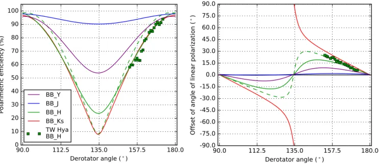
The left-hand panel of Figure4shows the polarimetric efficiency curves against derotator angle (θder) for the four broadband filters
of IRDIS. The solid lines show the polarimetric efficiency de-rived from the Mueller matrix model for the optical system for 90◦ ≤ θ
der ≤ 180◦, while the green dashed line shows this for
0◦ ≤ θder ≤ 90◦inH-band only. These green solid and dashed
curves clearly do not overlap, and the same is true for the other filters (not shown). This asymmetry acrossθder =90◦in the
po-larimetric efficiency curve is caused by a non-ideal behavior of HWP2, i.e. the retardance, λ/2 (see Paper II). A dramatic
de-crease in polarimetric efficiency is seen forθder≈45◦and 135◦
90.0
112.5
135.0
157.5
180.0
Derotator angle ( )
0
10
20
30
40
50
60
70
80
90
100
Polarimetric efficiency (%)
BB_Y
BB_J
BB_H
BB_Ks
TW Hya
BB_H
90.0
112.5
135.0
157.5
180.0
Derotator angle ( )
-90.0
-75.0
-60.0
-45.0
-30.0
-15.0
0.0
15.0
30.0
45.0
60.0
75.0
90.0
Of
fse
t o
f a
ng
le
of
lin
ea
r p
ola
riz
at
ion
(
)
Fig. 4. Left: Polarimetric efficiency as a function of derotator angle for all broadband filters listed in Table1. The green squares show theH-band
polarimetric efficiencies measured for TW Hydrae scaled to the model curves (Sect.5.3). The green dashed curve shows the model polarimetric efficiency for the range 0◦≤θder≤
90◦
inHband. This filter shows the strongest asymmetry aroundθder=90◦
, which is caused by the non-ideal retardance of HWP2.Right: The model polarization angle offset plotted againstθderfor the same filters (solid and dashed lines; as before, the dashed line covers the range 0◦≤θder≤
90◦
). In the ideal case, the polarization angle offset would remain 0◦
. However, there is a clear dependency onθderforHandKsband, and to a lesser extend forYband, while theJband remains close to ideal. The polarization angle offsets measured as φ0for TW Hydrae are plotted as green squares. The deviation of the on-sky data from the model curves is caused by the crosstalk contribution of other optical components.
ideal< 4◦; it is<11◦ inY, and can reach up to 34◦ inH. For
Ksband, the polarization angle offset does not even return to its
equilibrium and continues rotating beyond±90◦(where a
rota-tion of+90◦is indistinguishable from−90◦).
The strong dependence of the polarization angle offset and polarimetric efficiency on θder inH and Ks band are
predom-inantly caused by crosstalk induced by the retardance of the derotator, which is close to that of a quarter-wave (λ/4) plate at these wavelengths. With these retardances, the derotator causes a strong linear to circular polarization crosstalk. This crosstalk means that when we use the wrong observing strategy we can lose up to 95% of incident linearly polarized signal, which is ultimately the information carier we aim to measure. Because other optical components (e.g., HWP2) contribute to this loss of polarization signal as well, we list the polarimetric efficiencies for the least favorable instrumental configuration in Table2.
Table 2.Lowest polarimetric efficiencies reached at the least favorable
instrumental set-up. The values are determined with the polarimetric instrument model (Paper II) for the broad-band filters described in Ta-ble1.
Y(%) J(%) H(%) Ks(%)
54 89 5 7
5.2.3. The telescope and SPHERE’s first mirror
On April 16, 2017, UT3’s M1 and M3 have been recoated, re-sulting in a more effective cancellation of IP when M3 and M4 are in crossed configuration (when looking at or close to zenith). Therefore, we present the lowest and highestIPvalues for each broadband filter as measured before and after recoating in Ta-ble3.
Table 3.IP(in percent of the total intensity) induced by the telescope
mirrors and M4 before and after recoating of the M1 and M3. The val-ues are shown at optimal, nearly crossed configuration of the reflection planes of M3 and M4 (ata=87◦
, withathe altitude angle of the Unit Telescope), and worst, close to aligned reflection planes (a=30◦
: the lowest altitude at which the ADC can correct for atmospheric disper-sion) for the IRDIS’ broadband filters.
Date a(◦) Y(%) J(%) H(%) K
s(%)
Before 87 0.58 0.42 0.33 0.29
16-04-2017 30 3.5 2.5 1.9 1.5
After 87 0.18 0.12 0.07 0.06
16-04-2017 30 3.0 2.1 1.5 1.3
5.3. Explaining TW Hydrae data with the instrument model
During the observation of the 20 HWP cycles, the derotator has rotated fromθder=173.2◦ toθder=152.6◦ (∆θder=−20.6◦). To
account for the variation of the measured AoLP between the HWP cycles, we have determined the correct value for the polar-ization angle offsetφ0for each cycle separately, based on the
as-sumption that the polarization is oriented in azimuthal direction, and thereforeUφ should be 0. We have achieved this by com-puting the sum over the absolute signals measured for the pixels in a centered annulus in theUφimage for a range ofφ0 values:
cUφ(φ0). We have selected theφ0value which yielded the lowest
cUφ(φ0). We have derived the relative polarimetric efficiency by
measuring the absolute signal over an annulus in theQφimage for each cycle, and dividing these values by that of the highest (coincidentally the first) HWP cycle. During the observing se-quence of TW Hydrae the polarimetric efficiency has decreased with∼40%.
55 60 65 70 75 80 85 90 95 100
Polarimetric efficiency (%)
Fit. BB_H TW Hya BB_H
Derotator angle (◦)
10 8 6 4 2 0 2 4
Residuals (%)
155.0 157.5 160.0 162.5 165.0 167.5 170.0 172.5 175.0
152.5
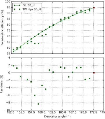
Fig. 5. Top: Polarimetric efficiency modeled (solid line) for the
same derotator and HWP2 angles as used during the observation of TW Hydrae (squares). Note that the polarimetric efficiencies measured for the HWP cycles of TW Hydrae are only determined relative to the other HWP cycles. We therefore scaled all data points such that the first cycle (red square, with the highest polarimetric efficiency) matches the value of the model.Bottom:Residuals between the model and the po-larimetric efficiencies obtained for TW Hydrae.
panel) for the TW Hydrae measurements. For this dataset we know neither the incident nor measuredPL(instead, we measure
Qφ ≈ PIL and do not knowI of the disk) to determine the
ab-solute value of the polarimetric efficiency. However, during the observations, Qφ is expected to be linearly proportional to the polarimetric efficiency. Therefore, we have measured for each HWP cycle the meanQφin a fixed annulus around the star and scale the images such that the highest mean value (from the first HWP cycle) matches the model’s polarimetric efficiency inH.
Although the polarimetric efficiency is rather well explained with the H-band model curve (green solid line), the polariza-tion angle offset deviates from the model. The models shown in Fig.4are created for the simplest configuration, where all instru-ment settings have been kept constant exceptθder, while during
the on-sky observations many optical components have changed position due to their field-tracking laws, such as HWP2 and the telescope altitude angle.
To account for these additional changes in configuration, we use the instrument model to compute the polarimetric efficiency and polarization angle offset for the same instrument configuration as was used during the observations of TW Hy-drae. We compare the predicted polarimetric efficiencies and polarization angle offsets with on-sky observation polarimetric efficiencies in Fig.5and polarization angle offsets in Fig.6.
The model predictions are very succesful at explaining the changes in polarimetric efficiency and polarization angle. We see some clear outliers in both Figs.5and6atθder ≈139◦, which
are most likely caused by a poor fit ofφ0for these HWP cycles.
This shows that our comparison is limited by the accuracy of the
0 5 10 15 20 25 30
Offset of angle of linear polarization (
◦)
Fit. BB_H TW Hya BB_H
Derotator angle (◦)
3 2 1 0 1 2 3 4
Residuals (
◦)
155.0 157.5 160.0 162.5 165.0 167.5 170.0 172.5 175.0
152.5
Fig. 6. Top:Expected polarization angle offsets of the same model
(solid line) as used in Fig.5; and the polarization angle offset angles (φ0 of Eq.17) of TW Hydrae (squares) with respect to azimuthal polariza-tion.Bottom:Residuals between the model polarization angle offsets andφ0retrieved for TW Hydrae.
polarimetric efficiency measurement in the data rather than that of the model.
6. Comparison between data reduction with
U
φ minimization and model-based correctionAfter Sect.5.1we paused our post-processing of the data to ana-lyze the instrumental polarization effects that cause the detected variations inPLandAoLPfor TW Hydrae in Sect.5.2and5.3.
We have succesfully implemented these lessons to create a de-tailed polarimetric instrument model and a model-based correc-tion method for the instrumental polarizacorrec-tion effects (see Pa-per II). In this section we will compare post-processing based on this correction method with the best post-processing we have performed without using the correction method, where we have corrected for residual IP empirically by minimizing signal in
Uφ. We will continue with the empiric correction method from where we stopped in Sect.5.1.
6.1. Refining the reduction by minimizingUφ
We determineφ0as described in Sect.5.3. Then we improve our
centering by shifting theQIPSandUIPSimages with a range ofx
andy steps to find the minimum cUφ(x, y) value. Because the
improved centering will affect the minimization process with which we found φ0, we repeat the minimization ofcUφ(φ0) on
the centered data, and find φ0 with increasing values between
6◦ ≤φ
0≤25◦for the 20 HWP cycles. A finalUφminimization
is performed to enhance ourIPcorrection: we find the minimum ofcUφ by searching a grid of constantsciQandc
j
Uwith which we
re-Qphi
scaled with r
0
scaled with r
2
Uphi
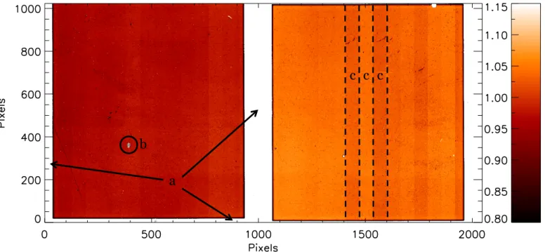
Fig. 7. FinalQφ(left) andUφ(right) images of TW Hydrae. BothQφandUφare displayed with identical linear scale, and either unscaled (top) or
scaled withr2(bottom) to compensate for the decrease of stellar flux with distance. All four panels are shown with North up and East to the left
for the same field of view of 4.900×
4.900
or up to a separation ofr=2.4500
from the star in both RA (−x-axis) and Dec (+y-axis).
spectively. For each point (i,j) in the grid, we computeUφwith Eq.16and addopt theci
Q andc
j
U values that yield the smallest
value ofcUφ.
TheUφminimizations are performed andQφ&Uφare com-puted per HWP cycle. At this stage we determine the polarimet-ric efficiency as described in Sect.5.3. The finalQφ&Uφimages shown in Fig.7are created by median combining the 20Qφand
Uφimages determined per cycle, respectively.
6.2. Correcting observations with the instrument model
In Sect.5.3 we show that the polarimetric instrument model can very well explain the variations in PL andAoLPmeasured
in the data as instrumental polarization effects. In Paper II, we have presented a highly-automated data-reduction pipeline (IR-DAP) that contains a correction method based on this instru-ment model. We have reduced the TW Hydrae data with IRDAP, without any prior correction for instrumental polarization effects (i.e. we did not apply Eqs.13and14orUφminimization). For il-lustrative purposes, we have also applied the model correction to three individual polarimetric cycles withθder = 169.7◦,162.0◦,
and 154.1◦ of this dataset. Fig.8shows the images as reduced with the method described in Sect.6.1and the result of the IR-DAP corrections. The QIPS images of these three HWP cycles
reduced withUφminimization are shown in panels a1, a2 and a3, the finalQφandUφimages of this reduction method are shown in panels b1 and b2, respectively. TheQimages for the same HWP cycles of panel a are shown after application of the correction
method in panels c1, c2 and c3, and the final IRDAP-reduced
QφandUφimages are shown in panels d1 and d2, respectively.
6.3. Comparison of reduction methods
While theQIPS images of Fig.8a show the rotation of the
but-terfly (φ0 , 0) caused by crosstalk, the correctedQimages of
panel c are clearly oriented such that φ0 ≈ 0◦. Although the
IRDAP-correctedQimages display a surface brightness which is approximately the same for all three images in panel c, the loss of polarization signal in the threeQIPS images (from a1 to
a3) is still visible as a decrease of the signal-to-noise ratio when comparing panel c3 with c1.
The azimuthal direction of the true polarization angle was used as an assumption in our reduction ofQφin Sect.6.1. There-fore, we cannot claim to have derived the angle of linear polar-ization in panel b1. However, since we do not need to assume a-priori knowledge aboutAoLPto compute the finalQφimage of panel d1, we can confidently claim to have determined theAoLP. As a result, theUφimage of panel d2, created withφ0 = 0◦ is
even cleaner (especially at small separations) than theUφimage of panel b2.
Although theQφimages produced with both methods (Fig.8
a1)
c1)
a2) a3)
c2) c3)
b1)
d1)
b2)
d2)
Fig. 8. a1, a2,&a3)QIPSimages of three HWP cycles withθder=169.7◦,162.0◦, and 154.1◦, respectively. These images are created with theUφ
minimization method (Sect.6.1). We can clearly see the buttefly patterns rotate in clockwise direction and the signal decrease from left to right.b)
When we use the assumption of azimuthal polarization, we can find the correctφ0for each HWP cycle and compute the finalr2-scaledQ
φ(b1) and
Uφ(b2) images (Sect.6.1). Because we have used the assumption that we know the Angle of Linear Polarization at each point, we cannot claim to have determined theAoLPin this image.c)When we apply the correction method to theQandUimages, we retrieve the best approximation of the incidentQandUimages (Sect.6.2). The displayedQimages (for the sameθderas panel a) contain the ideal orientation of the butterflies and are corrected for the reduced polarimetric efficiency. However, the latter does not improve the signal to noise (illustrated by the increased noise in panel c3).d1&d2)The IRDAP-correctedQφandUφimage. Because we no longer need the assumption that we know theAoLPa priori, we can useQandUafter the correction method to determine theAoLPin our final reduction.
method may suffice for a face-on disk such as TW Hydrae. How-ever, the loss of polarization signal as displayed between panels a1, a2 & a3 illustrates that our combination of data from multiple polarimetric cycles will result in very poorly constrained polari-metric intensity measurements. More importantly, when we ob-serve disks at larger inclination, especially inHorKsband, even
qualitative analysis of the data is likely to become skewed when the instrumental polarization effects are not corrected properly. In Paper II we illustrate that the shape ofQφand especiallyUφ images of the disk around T Cha look much more reliable (i.e. more similar to radiative-transfer model predictions,Pohl et al. 2017)) after applying the correction method.
7. Recommendations for IRDIS/DPI
7.1. Observing strategy to optimize polarimetric performance
Previous publications (e.g., Garufi et al. 2017) have demon-strated that the polarimetric mode of IRDIS is a very effective tool to image the scattering surface of protoplanetary and debris disks. However, the analysis of the TW Hydrae data presented in this paper illustrate that the polarimetric efficiency can be neg-atively affected when the instrument configuration is not opti-mized. When using IRDIS/DPI in field-tracking mode, we rec-ommend the following adjustments to the observing strategy to avoid a loss of polarized signal:
– When no strict wavelength requirements are present and the disk surface brightness is expected to be gray in the NIR: use
Jband to achieve a>90% polarimetric efficiency, which is nearly independent of the remaining instrumental setup.
– However, most young stars are red, causing their disks to scatter more light inH than in Jband. If the previous rec-ommendation to useJband cannot be met and theY-,H-, orKs-band filters are used, avoid the use of derotator angles
22.5.|θder|.67.5◦+n· 90◦, withn∈Z.
The latter recommendation ensures a polarimetric efficiency
≥70%. This constraint onθdercan be achieved with two simple
steps:
1. Within ESO’s Phase 2 Proposal Preparation tool (P2PP or P2), split the total observation within an observing block (OB) into parts (templates) where the difference between p
andadoes not vary by more than 90◦, resulting in|∆θ
der|<
45◦, becauseθder ∝(a−p)/2;
2. For each template, theθder constraint can be determined by
finding the average parallactic and altitude angles and apply-ing a derotator (position angle) offset of:
INS.CPRT.POSANG= <p−a>+n ·180◦, (18)
withn∈Z, and<>indicating the average values.
The parallactic and altitude angle can be determined by:
p = arctan sin (HA)
tan (φ) cos (δ)−sin (δ) cos(HA)
!
, (19)
a = arcsin (sin (δ) sin (φ)+cos (δ) cos (φ) cos (HA)), (20)
whereφ=−24.6◦is the latitude of the VLT at the Paranal obser-vatory,δis the declination of the star, andHAis the Hour Angle of the star=Local Sidereal Time (LST) - Right Ascension (RA). The required derotator offset will be strongly dependent on the exact start of the observation template. Duringvisitor mode
observations, where the observer is present at the observatory, the optimal derotator offset can be included in the OBs just be-fore the start of the observations. During remoteservice mode
position angle offsets to the README file of the OB, or by pro-viding LST constraints and a corresponding optimal derotator offset to the OB, preferably around a time when the parallactic angle does not change too much during the observation.
When the optimal value for INS.CPRT.POSANG is used, the mean θder lies at either 0◦ or 90◦, which orients the derotator
horizontal or vertical with respect to the Nasmyth platform. This orientation will cause little or no crosstalk and therefore limited loss of polarized signal and a close to ideal polarization angle.
20 30 40 50 60 70 80 90
Telescope altitude angle (
◦)
180
150
120
90
60
30
0
30
60
90
120
150
180
Pa
ra
lla
cti
c a
ng
le
of
ta
rg
et
(
◦
)
0
10
20
30
40
50
60
70
80
90
100
Polarimetric efficiency (%)
Fig. 9.The polarimetric efficiency inHband as a function of the
paral-lactic angle and altitude angle, when the derotator is in field-tracking mode without an additional derotator offset. The dashed line shows the parallactic and altitude angle of TW Hydrae across the sky, with the solid line showing the angles during the SPHERE observation. We clearly see that using default derotator settings (North up on the detec-tor) will give us mediocre polarimetric efficiencies.
Figure9shows the polarimetric efficiency mapped forpand
a without the application of a derotator offset. Given the path traveled by TW Hydrae during our observations shown with the black solid line (<p> ≈ 90◦, <a> ≈ 50◦), we could have avoided the loss of polarization signal by providing a derotator position angle offset of INS.CPRT.POSANG=90−50=40◦, rotating the derotator by 20◦. We did not apply this derotator
offset because we were not aware of the strong crosstalk for IRDIS/DPI at the time of these observations.
7.2. SPHERE design upgrades
7.2.1. HWPs 1 & 3 to reduce instrumental polarization effects
The most thorough way to reduce instrumental polarization effects for IRDIS would be to introduce two more HWPs in the optical path. A HWP1 at the same location as for ZIMPOL, in between M3 and M4, can keep theIPinduced by both mir-rors perpendicular to let them cancel out. We then use HWP2 in a slightly different fashion: rather than aligning the to-be-measured polarization angles with the analyzers, it aligns the desired polarization with the reflection plane of the derotator, as it does for ZIMPOL (Schmid et al. 2018). Similar to ZIMPOL, this new rotation law for HWP2 requires that we install a third HWP to align the desired polarization angle with the transmision axes of IRDIS’ polarizers. We recommend to install this HWP3 directly downstream of the derotator, to completely remove all crosstalk.
We are aware that the diverging beam downstream of the derotator is relatively large, which might make it difficult to produce a HWP that is large enough. The feasibility of this recommendation is yet to be determined. Alternatively, as for ZIMPOL, HWP3 could be installed further down the optical path when the beam starts to become smaller (e.g., between the apodizer wheel and the DTTS beam splitter, before large incidence-angle reflections are encountered by the beam).
7.2.2. Recoating of the derotator to reduce retardance
As we describe in Sect.5.2.2, due to its unfavorable retardance (nearlyλ/4 inHandKs) the derotator is by far the largest
con-tributor of crosstalk and hence loss of polarimetric efficiency. Therefore, an alternative recommendation to reduce the loss of polarimetric efficiency for IRDIS is to recoat the three mirrors of the derotator with a coating that yields a total retardance of the derotator close toλ/2 in all filters. We are currently investigat-ing the feasibility to apply a coatinvestigat-ing to the derotator that yields
∼λ/2 retardance over the very broad wavelength range required by ZIMPOL and IRDIS combined. Whether HWP3 is still de-sired after recoating depends on how close the retardance of the new coating is to the ideal value for the full wavelength range covered by IRDIS.
7.2.3. A polarizing beam splitter to increase throughput
The throughput of the combination of non-polarizing beam splitter plate+ wire-grid polarizers is ∼50%, as discussed in Sect.3.3. Replacing the non-polarizing plate with apolarizing
beam splitter plate will immediately increase the throughput with a factor∼2. An additional result of this upgrade will also be that polarimetry is offered ’for free’ for any observation per-formed with IRDIS. Polarimetry-for-free will allow a substan-tial boost of the science output of the instrument by serendipi-tous discoveries of polarized circumstellar disks during planet-hunting surveys. The observer can choose whether to use full HWP cycles if polarimetry is not the primary objective. How-ever, one should always consider at least cycling two HWP an-gles set 45◦apart (e.g.,Q±), especially for DBI to avoid confus-ing polarized signal for a spectral feature. This necessity of the HWP requires that we need to investigate whether inlcuding this optical component affects the contrast of DBI, classical imaging, but also IFS observations.
7.2.4. IRDIS polarimetry & IFS observations simultaneously