Volume 36, Number 2, Pages 135–249 S 0273-0979(99)00776-4
Article electronically published on February 19, 1999
ANALYTIC AND GEOMETRIC BACKGROUND OF RECURRENCE AND NON-EXPLOSION OF THE BROWNIAN
MOTION ON RIEMANNIAN MANIFOLDS
ALEXANDER GRIGOR’YAN
Abstract. We provide an overview of such properties of the Brownian
mo-tion on complete compact Riemannian manifolds as recurrence and non-explosion. It is shown that both properties have various analytic characteri-zations, in terms of the heat kernel, Green function, Liouville properties, etc. On the other hand, we consider a number of geometric conditions such as the volume growth, isoperimetric inequalities, curvature bounds, etc., which are related to recurrence and non-explosion.
Contents
1. Introduction 136
Acknowledgments 141
Notation 141
2. Heat semigroup on Riemannian manifolds 142
2.1. Laplace operator of the Riemannian metric 142 2.2. Heat kernel and Brownian motion on manifolds 143
2.3. Manifolds with boundary 145
3. Model manifolds 145
3.1. Polar coordinates 145
3.2. Spherically symmetric manifolds 146
4. Some potential theory 149
4.1. Harmonic functions 149
4.2. Green function 150
4.3. Capacity 152
4.4. Massive sets 155
4.5. Hitting probabilities 159
4.6. Exterior of a compact 161
5. Equivalent definitions of recurrence 164
6. Equivalent definitions of stochastic completeness 170
7. Parabolicity and volume growth 174
7.1. Upper bounds of capacity 174
7.2. Sufficient conditions for parabolicity 177 8. Transience and isoperimetric inequalities 181
9. Non-explosion and volume growth 184
Received by the editors October 1, 1997, and, in revised form, September 2, 1998. 1991Mathematics Subject Classification. Primary 58G32, 58G11.
Research supported by the EPSRC Fellowship B/94/AF/1782 (United Kingdom). c
1999 American Mathematical Society
10. Transience andλ1 191
10.1. The first eigenvalue 191
10.2. Faber-Krahn inequality and transience 192
10.3. Heat kernel’s upper bound 195
11. Transience and volume growth 197
11.1. Relative Faber-Krahn inequality 197
11.2. Covering manifolds 199
12. Transience on manifolds with a pole 200
13. Liouville properties 203
13.1. Lp-sub(super)harmonic functions 204
13.2. Liouville property for Schr¨odinger equation 205
13.3. Bounded harmonic functions 208
13.4. Minimal surfaces 209
13.5. Liouville property on Riemannian products 209 14. Harmonic functions on manifolds with ends 212
14.1. Parabolic subsets and ends 212
14.2. Spaces of harmonic functions on manifolds with ends 213
14.3. Manifolds with regular ends 214
14.4. Non-parabolicity of regular ends 216
15. Curvature and comparison theorems 220
15.1. Mean curvature 220
15.2. Sectional and Ricci curvature 223
15.3. Parabolicity for two dimensional manifolds 227 16. Heat kernel’s lower bounds and recurrence ofα-process 232 17. Escape rate as a measure of transience 234
18. Problem section 236
References 242
1. Introduction
The irregular movement of microscopic particles suspended in a liquid has been known since the beginning of the nineteenth century. In 1828, English botanist Robert Brown published his observations of ceaseless erratic motion of pollen grains in water. He emphasized the universal character of the phenomenon in contrast to the previous belief which attributed it to vital nature. That was the discovery of the physical phenomenon which was later namedthe Brownian motion.
It was not until 1905 when the effect was explained by Albert Einstein [56] as the result of the irregular collisions that the fine particles in suspension experience from molecules. Einstein realized the stochastic nature of the Brownian motion and proved that the probability distribution of the displacement of a Brownian particle satisfied a diffusion equation. Moreover, he computed the diffusion coefficient D and made a prediction that the mean displacement of the particle during a time t was√2Dt. The latter was confirmed experimentally by Jean Perrin in 1908 which later brought him a Nobel prize. That work was a strong argument in favor of the molecular-kinetic theory of heat and even the atomic structure of matter.
The simplest mathematical model of the Brownian motion is a random walk on a lattice. Suppose that a particle moves on the nodes of Zd as follows. At each
Figure 1. The random walk onZ2
Figure 2. The Brownian motion onR2
step, it chooses randomly one of the 2dneighboring nodes, with equal probability (2d)−1, and jumps to that node (see Figure 1).
A natural question is what happens with the particle as the number of steps n → ∞? On average, the displacement of the particle is of the order √n as in Einstein’s model, but this does not say much aboutthe trajectory of the particle. Since the rule of the movement of the particle is homogeneous and isotropic, one may expect that, in a long run, the number of moves in all 2d directions should be approximately the same, and the particle should be regularly returning to a neighborhood of the origin. However, this is wrong! G.P´olya [159] discovered in 1921 that a long term behavior of the random walk depends on the dimensiond. If d≤2 then the particle does visit every node (including the origin) infinitely many times, with probability 1. However, ifd >2 then the particle visits every node only finitely many times, also with probability 1.
In other words, an observer of the two-dimensional random walk could see the particle in his/her range at arbitrarily large moments of time, whereas in the three-dimensional space, the particle will escape from any bounded region after some time forever. The first type of behaviour of the particle is referred to asrecurrence whereas the second one is calledtransience.
The same phenomenon takes place for a continuous time Brownian motion in Rd which can be obtained from the random walk on Zd as a limit by a proper
refinement of the lattice and the time step. A rigorous construction of a continuous model of the Brownian motion was done by Norbert Wiener [189]. This process is called the Wiener process and is recognized now as the standard model for the Brownian motion. Henceforth, we will use the term “the Brownian motion” as a synonym for the Wiener process (see Figure 2).
One of the goals of this paper is to study the geometric background of the property of the Brownian motion to be recurrent or transient. In other words, what geometric properties of the state space causes the trajectory of the stochastic process to return to any region at arbitrarily large times or to leave any bounded region forever?
The answer to this question depends on the family of the state spaces in question. In the category of the Euclidean spaces (or lattices) one may answer that it is the dimension which makes the difference. However, this becomes totally wrong in the category ofRiemannian manifolds. A Riemannian manifold is an abstract version of a smooth curved surface. This is rather a point of view that takes into account only intrinsic properties of the surface, which do not depend on the embedding space.
Riemannian manifolds provide rich enough family of geometries. For example, all classical model geometries - the spherical, euclidean and hyperbolic geometries - are particular cases of Riemannian geometries. It turns out that the continu-ous Brownian motion can be constructed on any Riemannian manifold (imagine a Brownian particle moving on a curved surface). The Brownian motion on a Rie-mannian manifold is called recurrent if it visits any open set at arbitrarily large moments of time with probability 1,andtransient otherwise.
We shall see that recurrence is related to various geometric properties of the underlying Riemannian manifold such as the volume growth, isoperimetric inequal-ities, curvature etc. On the other hand, recurrence happens to be equivalent to certain potential-theoretic properties ofthe Laplace operator on the manifold. For example, the recurrence of the Brownian motion inR2is linked to the fact that the fundamental solution log|x|of the Laplace operator inR2 is signed as opposed to the positivity of the fundamental solution|x|2−d inRd, ford >2.
The question of recurrence of the Brownian motion on Riemann surfaces goes back to the uniformization theorem of F.Klein, P.Koebe and H.Poincar´e. This celebrated theorem says, in particular, that any simply connected Riemann surface is conformally equivalent to one of the following canonical surfaces:
1. the sphere (surface of elliptic type)
2. the Euclidean plane (surface of parabolic type) 3. the hyperbolic plane (surface of hyperbolic type).
The problem of deciding what is the type of a given Riemann surface is known as the type problem. It is easy to distinguish between the elliptic type and the others - the former is compact whereas the latter are not. A more interesting question is how to distinguish the parabolic and hyperbolic types by using intrinsic geometric properties of Riemann surfaces. Amazingly, the parabolicity is exactly equivalent to the recurrence of the Brownian motion on the Riemann surface in question.
The understanding of parabolicity of Riemann surfaces from the potential -theoretic point of view is largely due to L.Ahlfors [1] - [3], P.J.Myrberg [144], R.Nevanlinna [149], [150] and H.Royden [163]. J.Deny [47], G.Hunt [98] and S.Kakutani [105] contributed to the potential-theoretic background of recurrence. The study of recurrence in connection with the geometry of Riemannian manifolds was boosted by the works of S.Y.Cheng and S.-T.Yau [28] and N.Varopoulos [183], [184].
Another property of the Brownian motion to be considered in this paper is stochastic completeness. This is a property of a stochastic process to have infinite
lifetime. In other words, a process is stochastically complete if the total probability of the particle being found in the state space is constantly equal to 1.This is also referred to as a conservation property (of probability) or non-explosion. Despite the fact that the very term “a probability measure” means a measure with the total mass 1, there are simple examples of stochastically incomplete processes. Consider a Brownian motion in a bounded region Ω ⊂ Rd with an absorbing boundary.
After hitting the boundary∂Ω,the particle dies, and this happens with a positive probability. Therefore, at any positive time, the total probability of the particle being found in Ω is smaller than 1.
The Brownian motion inRd (and the standard random walk in Zd) is
stochas-tically complete. One might wonder whether stochastic incompleteness has to do only with the presence of some killing conditions. It turns out that even with-out any killing, there may exist ageometric reason for stochastic incompleteness. R.Azencott [6] showed that the Brownian motion on a Riemannian manifold M may be stochastically incomplete even ifM is geodesically complete. Note that a bounded region Ω⊂Rdis not geodesically complete when considered as a manifold. In the example of R.Azencott, the manifoldM has a negative sectional curvature which grows fast enough to−∞with the distance from an origin. The stochastic incompleteness of the Brownian motion onM occurs because negative curvature on a manifold plays the role of a drift to infinity, and a very high negative curvature may produce an extremely fast drift which sweeps a Brownian particle to infinity in a finite time.
An interesting question is to understand precisely what geometric properties of M ensure stochastic completeness or incompleteness of the Brownian motion. The crucial contributions here are due to R.Azencott [6], M.Gaffney [66], R.Khas’minskii [111] and S.-T.Yau [194].
One may wonder what recurrence and the conservation property have in com-mon. Both transience and explosion (=stochastic incompleteness) reflect the ten-dency of the Brownian motionto escape to infinity. While transience says that the Brownian motion escapes to infinity, explosion means that it does it in a finite time. There is a full range of variousescape rates between transience and explosion. No wonder that many conditions of recurrence of Brownian motion on manifolds have their counterparts for stochastic completeness.
The purpose of this paper is to expose the relationship between recurrence and the conservation property on the one hand, and many other geometric and potential-analytic properties on the other hand. For example, recurrence can be characterized in terms of a fundamental solution to the Laplace equation, superharmonic func-tions, capacities, the heat kernel, the Liouville property for certain Schr¨odinger equation, etc. The stochastic completeness can also be characterized in various terms including the uniqueness in the Cauchy problem for the heat equation in the class of bounded solutions. Given that much, these two properties of the Brownian motion appear to be of fundamental importance for analysis on manifolds and for adjacent areas.
This paper splits into two parts. The first part consists of sections 2 - 9 and is rather elementary. It focuses on the one hand on Theorems 5.1 and 6.2, which con-tain various characterizations of transience and explosion partly already mentioned above, and on the other hand on Theorems 7.3 and 9.1, which give the follow-ing sufficient conditions for recurrence and non-explosion in terms of the volume growth.
Let V(r) denote the Riemannian volume of a geodesic ball of radius r with a fixed center. Then the Brownian motion on a geodesically complete manifoldM is recurrent provided
Z ∞
rdr V(r) =∞.
For example, this condition is satisfied ifV(r)≤Cr2. In particular, this explains why the Brownian motion onR2 is recurrent - there is just not enough volume in the two-dimensional Euclidean space!
Furthermore, the Brownian motion onM is stochastically complete provided
Z ∞
rdr
logV(r) =∞.
For example, this condition is satisfied if V(r)≤exp(Cr2). Clearly, all Euclidean spaces fit into this volume growth. This explains why we have to move to manifolds in order to observe stochastic incompleteness -Rd is too small for that!
Full proofs of the key results of the first part are provided, which should be accessible for graduate students with adequate background. Let us emphasize that we normally assume known (and, thus, do not provide proof for) all facts which depend only on the local structure of the manifold. For example, we freely use such properties of solutions to the elliptic equations asC∞-regularity, convergence principles, maximum principle, solvability of the Dirichlet problem etc. On the contrary, we concentrate on the properties related to the structure of the manifold “in the large”.
The second part is devoted to the relations of recurrence and non-explosion to other questions such as Liouville properties, heat kernel bounds, eigenvalues of the Laplace operator, curvature, escape rate of the Brownian motion, etc. This part is more advanced and sketchy, and some results may appear to be new even to the experts. However, we do not aim to include the most recent and general results, and we have opted for those which exhibit interesting phenomena without technical complications.
The subject of this paper lies on the borderline between different fields of math-ematics such as Riemannian Geometry, Stochastic Analysis, Partial Differential Equations and Potential Theory. We refer the reader to the following textbooks for the necessary background:
• Riemannian Geometry: [22], [21], [112], [158], [169].
• Analysis and PDE: [43], [68], [116], [134], [188].
• Probability: [55], [60], [103], [133], [136], [172].
• Potential Theory: [16], [30], [32], [51], [64], [179].
The following monographs and survey articles provide additional valuable infor-mation about elliptic and parabolic differential equations on manifolds: [5], [69], [92], [130], [140], [113], [161], [162], [167], [170], [180].
There is also a vast literature devoted to recurrence criteria for random walks on graphs and lattices. We do not touch this question here and refer an interested reader to the books [53] and [191] as well as to the surveys [67], [90], [166], [190].
Acknowledgments
The author is obliged to Mike Cranston, Thierry Coulhon, Minoru Murata and Laurent Saloff-Coste for numerous suggestions for improving the original manu-script. He is also grateful to David Hoffman and Robert Osserman for their interest in this work and for encouragement.
Notation
The following list of notation is provided for convenience of reading. Most of them are also explained in the main body of the paper.
M - a smooth connected Riemannian manifold. In many cases,M is geodesically complete and non-compact.
d≥2 - the (topological) dimension ofM.
dist(x, y) - the geodesic distance onM between the points x, y∈M. µ- the Riemannian volume onM.
µ0 - the Riemannian measure of the co-dimension 1 on hypersurfaces inM.
|A| := µ(A) or µ0(A) depending on the context (for example, if A is an open subset ofM, then|A|=µ(A); whereas ifA is a boundary of an open subset, then
|A|=µ0(A) ).
B(x, r) - the geodesic ball of radiusrcentered at the point x∈M. V(x, r) :=µ(B(x, r) ) - the volume growth function.
∆ - the Laplace -Beltrami operator onM.
λ1(Ω) - the first eigenvalue of the Dirichlet problem for ∆ in Ω (where Ω is a region inM).
p(t, x, y) - the heat kernel associated with the operator 12∆.
pΩ(t, x, y) - the heat kernel in the region Ω with the Dirichlet boundary condition on∂Ω.
Pt - the heat semigroup with the kernelp(t, x, y).
PtΩ- the heat semigroup with the kernelpΩ(t, x, y).
G(x, y) - the Green kernel of−∆ onM.
GΩ(x, y) - the Green kernel of−∆ in the region Ω with the Dirichlet boundary condition.
Xt - the Brownian motion onM generated by 12∆.
Px, Ex - measure and expectation, respectively, on the space of paths of the
Brownian motion started atx∈M.
bΩ,sΩ - the subharmonic and superharmonic potentials of an open set Ω - see Section 4.4.
eF,hF - the hitting probabilities - see Section 4.5.
C0∞(Ω) - the set of smooth real-valued functions on Ω with compact support in Ω.
L(K,Ω) - the set of locally Lipschitz functionsφonM, compactly supported in Ω and such that 0≤φ≤1 andφ|K= 1.
{Ek}- an exhaustion sequence onM - see Section 4.2.
x→ ∞- a sequence {xk} onM which leaves any compact set after somek. If M is geodesically complete, then this is equivalent to dist(x, o)→ ∞where ois a reference point.
flux
Γ f - the flux of the function f through a smooth oriented hypersurface Γ, that is, RΓ∂f∂νdµ0 where ν is a unit normal vector field on Γ associated with the
orientation of Γ. If Γ is a boundary of an open set Ω, thenν points outwards from Ω.
Sd - thed-dimensional unit sphere inRd+1.
Hd- thed-dimensional hyperbolic space.
ωd - the boundary area of the unit sphere inRd.
const - a positive constant which may be different at different occurrences. 2. Heat semigroup on Riemannian manifolds
The simplest way to construct Brownian motion on a Riemannian manifoldM is to construct firstthe heat kernel which will also serve as the density of the transition probability. The heat kernel will be denoted byp(t, x, y) wheret >0 is a time,x, y are points onM. Thus, the probability that the Brownian motion starting at the pointxlies in a measurable set Ω⊂M at the timetis given by
Z
Ω
p(t, x, y)dµ(y). InRd,the heat kernel is given by the classical formula
p(t, x, y) = 1 (2πt)d/2
exp −|x−y| 2 2t
!
. It is known to satisfy the heat equation
∂p ∂t −
1
2∆p= 0 (2.1)
in the variables (t, x) (the pointy is considered as fixed) and the initial data p(t,·, y) −→
t→0+δy (2.2)
whereδy is the delta function of Dirac.
The properties (2.1) and (2.2) can be used to define the heat kernel on an arbi-trary Riemannian manifoldM, which is done below.
2.1. Laplace operator of the Riemannian metric. Letgij be the Riemannian
metric tensor on M. This means that, in any coordinate chart (x1, x2, ..., xd) on
M, the length element can be computed by ds2=gijdxidxj
where we assume the summation on the repeated indices. Denote by gij the
el-ements of the inverse matrix kgijk−1 and let g := detkgijk. Then the Laplace
operator ∆ associated with the metricgij is defined by
∆ = √1 g
∂ ∂xi
√
ggij ∂ ∂xj
. (2.3)
This is a second order elliptic operator on M. It is possible to show that (2.3) defines the same operator in different charts.
Sometimes it is useful to represent the Laplacian in the form ∆ = div∇
where the gradient∇acts on a functionf by (∇f)i=gij ∂f
and the divergence div acts on a vector fieldF =Fi ∂∂xi by
divF =√1 g
∂ ∂xi
√gFi.
Green’s formula, which follows easily from Stokes’s theorem, says that, for any precompact regionU and for any functions u, v∈C02(U),
Z U
v∆u dµ=−
Z U
∇v∇u dµ , (2.4)
where∇v∇uis the inner (Riemannian) product of the vectors
∇v∇u=gij(∇u) i
(∇v)j=gij∂u ∂xi
∂v ∂xj,
anddµis the Riemannian volume element, which is defined by
dµ=√g dx1dx2... dxd. (2.5) If the boundary∂U is smooth enough (say,C1) andu, v∈C2(U)∩C1 U, then we have the following version of (2.4) with a boundary term
Z U
v∆u dµ=
Z ∂U
v∂u ∂νdµ
0−Z
U
∇v∇u dµ, (2.6)
wheredµ0 in the middle integral is the Riemannian volume element on the subman-ifold∂U, andν is the outward unit normal vector field on∂U.
2.2. Heat kernel and Brownian motion on manifolds. Any function on (0,∞)
×M ×M satisfying (2.1) and (2.2) is called a fundamental solution of the heat equation (2.1) on M. The heat kernel is the smallest positive fundamental solu-tion of the heat equasolu-tion on M. It was proved by J.Dodziuk [48] that the heat kernel always exists (regardless of geodesic completeness) and is smooth in (t, x, y). Moreover, the heat kernel possesses the following properties.
1. Symmetry inx, y, that isp(t, x, y) =p(t, y, x). 2. The semigroup identity: for anys∈(0, t)
p(t, x, y) =
Z M
p(s, x, z)p(t−s, z, y)dµ(z). (2.7) 3. For allt >0 andx∈M,
Z M
p(t, x, y)dµ(y)≤1. (2.8) As soon as one has (2.7) and (2.8), a (sub)Markov process Xt on M can be
constructed with the transition densitypby using the standard probabilistic tools (see [30], [55]). The processXtturns out to be a diffusion and is referred to asthe
Brownian motion orthe Wiener process on M.The corresponding measure in the space of paths emanating from a pointxwill be denoted byPx.
Given an open set Ω⊂M,one can treat Ω as a manifold itself. Let us denote by pΩthe heat kernel of Ω. Minimality of the heat kernel implies thatpΩvanishes on the boundary∂Ω, at least if∂Ω is smooth. This implies, in turn, thatpΩincreases on enlarging of Ω.
The way the global heat kernelpis constructed in [48] is the following: one first defines pΩ for precompact sets Ω (which can be done by using the eigenfunction expansion) and then lets
p:= lim
k→∞pΩk
where{Ωk}is an increasing sequence of precompact open sets with smooth bound-aries, which exhaustM.
Due to (2.7) and (2.8), the heat kernelp(x, y, t) can be considered as a kernel of the submarkovian operator semigroupPtwhich acts on functions onM by
Ptf := Z
M
p(·, y, t)f(y)dµ(y).
The semigroup corresponding to pΩ will be denoted by PtΩ. If f is a continuous
bounded function on M, then the function u(x, t) := Ptf(x) solves the Cauchy
problem inM×(0,∞):
∂u ∂t =
1 2∆u , u(·,0) =f .
Moreover, iff ≥0 thenPtf is the smallest non-negative solution to this problem.
See [171] for detailed properties of the heat semigroup on manifolds.
Let us briefly mention another way of constructing the heat kernel on Riemannian manifolds which goes back to Gaffney [65] and which was implemented in full generality by Cheeger and Yau [27]. The idea is to consider ∆ as an unbounded operator inL2(M, µ). It is possible to prove that the operator ∆ with the domain C0∞(M) is essentially self-adjoint and non-positive. Therefore, by using the spectral theory, one can construct the one-parameter operator semigroup e12t∆ acting in L2(M, µ). Next, one proves that this semigroup possesses a smooth kernel which is the heat kernel (see also [162], [169, p.94]). The equivalence of these two approaches was proved in [48].
Other methods of constructing the Brownian motion on manifolds (or even on more general underlying spaces) can be found in [6], [57], [63], [102], [133], [136].
Now we can precisely define the recurrence and conservation properties. Definition 2.1. Brownian motion Xt on a manifold M is recurrent if, for any
non-empty open set Ω and for any pointx∈M,
Px{there is a sequencetk → ∞such thatXtk∈Ω}= 1.
OtherwiseXtis transient.
Definition 2.2. Brownian motion Xt is stochastically complete (=possesses the
conservation property or the non-explosion property) if, for allx∈M andt >0,
Z M
p(t, x, y)dµ(y) = 1
(in other words,Pxis a probability measure in the sense that its total mass is equal
to 1).
It is convenient to say that a manifold is stochastically complete (recurrent, transient) when the Brownian motion on it has this property.
2.3. Manifolds with boundary. Sometimes it is useful to allow a manifold M to possess a boundary∂M. In this case, we assume that the heat kernelsp(t, x, y) and pΩ(t, x, y) satisfy in addition the Neumann boundary condition on ∂M and ∂M∩Ω respectively. For the Brownian motion this means thatXtreflects on∂M.
Most results of this paper remain true for manifolds with boundary. However, by default we consider manifolds without boundary in order to avoid some technical complications.
3. Model manifolds
The purpose of this section is to introduce a class of model manifolds which are the manifolds with rotational symmetry.
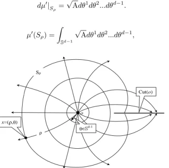
3.1. Polar coordinates. Let us fix a point o ∈ M and denote by Cut(o) the cut locus of o. Away from Cut∗(o) := Cut(o)∪ {o}, one can define the polar coordinates with the poleo(see Figure 3). Namely, for any pointx∈M\Cut∗(o) there corresponds a polar radiusρ:= dist(x, o) and a polar “angle”θ∈Sd−1such
that the shortest geodesics fromotoxstart atoto the directionθinToM. We can
identifyToM withRd so thatθ can be regarded as a point onSd−1. In particular,
M\Cut∗(o) is diffeomorphic to a star-like region onR+×Sd−1 (see [112] and [69] for proofs of the facts mentioned here).
The Riemannian metric inM\Cut∗(o) has in the polar coordinates the form ds2=dρ2+Aij(ρ, θ)dθidθj, (3.1)
where (θ1, θ2, ..., θd−1) are coordinates onSd−1andkA
ij(ρ, θ)kis a positive definite
matrix. In fact, Aij(ρ,·) is the Riemannian metric tensor on the geodesic sphere
Sρ :=∂B(o, ρ)\Cut(o). Denote A = detkAijk. Then we have, by (2.5), the area
element onSρ
dµ0|S
ρ =
√
Adθ1dθ2...dθd−1. (3.2) In particular,
µ0(Sρ) = Z
Sd−1
√
Adθ1dθ2...dθd−1, (3.3)
x=( , )
d-1
ρ
Cut(o)
o Sρ
x
ο
( )d
d
ds
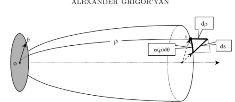
Figure 4. The metric on the surface of revolutionMσ
assuming thatθ1, θ2, ..., θd−1 are defined almost everywhere onSd−1.
It follows easily from (2.3) and (3.1) that the Laplace operator has in the polar coordinates the form
∆ = √1 A
∂ ∂ρ(
√
A ∂
∂ρ) + ∆Sρ =
∂2 ∂2ρ+
log√A
0 ∂
∂ρ+ ∆Sρ (3.4)
where (·)0 denotes∂/∂ρand ∆Sρ is the Laplace operator on the submanifoldSρ.
We say thatM isa manifold with a pole ifM possesses a pointowith an empty cut locus Cut(o). The point ois called the pole of M, and the polar coordinates are defined on M \ {o}. If, in addition, M is geodesically complete, then M is diffeomorphic toRd.
3.2. Spherically symmetric manifolds. In the next sections, we will introduce methods for determining whether a given manifold is recurrent or stochastically complete. The simplest class of manifolds where these methods apply and give straightforward answers is the class of spherically symmetric manifolds.
A manifold M with a pole o is called a spherically symmetric manifold or a model if the Riemannian metric onSρ (see (3.1)) is given by
Aij(ρ, θ)dθidθj=σ2(ρ)dθ2
where dθ2 is the standard Euclidean metric Sd−1 and σ(ρ) is a smooth positive
function ofρ. In other words, the Riemannian metric on Sρ is obtained by scaling
that ofSd−1 by the factorσ2.
Given a smooth positive function σ(ρ) on (0, R0), the necessary and sufficient condition that such a manifold exists is
σ(0) = 0 and σ0(0) = 1. (3.5) The hypotheses (3.5) ensure that the metric on the cone (0, R0)×Sd−1 defined by
ds2=dρ2+σ2(ρ)dθ2,
can be smoothly extended to the originρ= 0 (see [69]). We assume in the sequel that σ satisfies (3.5) and denote by Mσ the cone (0, R0)×Sd−1 with the added origin.
Clearly, the model manifoldMσ is diffeomorphic to an open ball inRdof radius
R0(or the wholeRdifR
0=∞). The metric on any geodesic sphere∂B(o, r) onMσ
is obtained from that ofSd−1by scaling it by the factorσ(r). In certain situations,
o
( , )
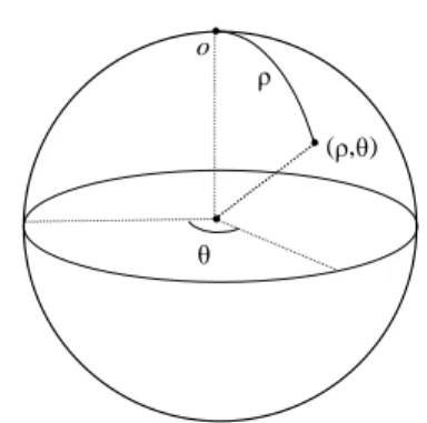
Figure 5. The polar coordinates onS2
Since√A =σd−1, we see from (3.3) that the boundary areaS(r) of the geodesic
sphere∂B(o, r) is computed by
S(r) =ωdσd−1(r),
whereωd is the area of the unit sphere inRd.The volumeV(r) of the ballB(o, r)
is given by
V(r) =
Z r
0
S(ξ)dξ=ωd Z r
0
σd−1(ξ)dξ.
The Laplace operator onMσ can be written down as follows (cf. (3.4))
∆ = ∂ 2
∂2ρ+ (d−1) σ0
σ ∂ ∂ρ+
1
σ2∆θ (3.6)
or
∆ = ∂ 2 ∂2ρ+
S0 S
∂ ∂ρ+
1
σ2∆θ (3.7)
where ∆θ denotes the Laplace operator on the sphere Sd−1. It is important that
the operator ∆θ does not depend on the variableρ.
The major examples of model manifolds are as follows. Example 3.1. IfR0=∞and
σ(r) =r, thenMσ is isometric toRd. The boundary area is
S(r) =ωdrd−1
and the Laplace operator is ∆ = ∂
2 ∂2ρ+
d−1 ρ
∂ ∂ρ+
1 ρ2∆θ. Example 3.2. Let us set
σ(r) = sinr.
ThenMσ is the sphereSd (assuming thatR0takes the maximum possible valueπ
and that the endpoint with ρ=π is added toMσ). If d= 2 thenr becomes the
The boundary area is
S(r) =ωdsind−1r .
The Laplace operator onSd acquires the form
∆ = ∂ 2
∂2ρ+ (d−1) cotρ ∂ ∂ρ+
1 sin2ρ∆θ,
where ∆θ is the Laplace operator on the sphereSd−1.This formula can be iterated
in the dimensiondto produce a full expansion of the spherical Laplace operator in the angular coordinates.
Example 3.3. Let us set
σ(r) = sinhr .
ThenMσis the hyperbolic spaceHd- the complete simply connectedd-dimensional
manifold with constant sectional curvature−1 (assumingR0=∞). The boundary area onHd is equal to
S(r) =ωdsinhd−1r
and the Laplace operator is ∆ = ∂
2
∂2ρ+ (d−1) cothρ ∂ ∂ρ+
1 sinh2ρ∆θ.
It turns out that recurrence and stochastic completeness of Mσ can easily be
determined via the boundary areaS(r). The following tests were proved by many authors in various settings ([1], [139], [111], [99], [100], [75]).
Proposition 3.1. Let Mσ be a model manifold with R0 = ∞ (so that Mσ is
geodesically complete and non-compact). Then Mσ is recurrent if and only if Z ∞
dr
S(r) =∞. (3.8)
Proposition 3.2. Let Mσ be a model manifold with R0=∞.Then M is stochas-tically complete if and only if
Z ∞
V(r)
S(r)dr=∞. (3.9)
The proofs will be given in Sections 5 and 6 respectively.1 The condition (3.8) holds for
S(r)≤constr, r→ ∞ and fails if
S(r)≥constr1+ε, ε >0.
This explains whyRd is recurrent ford≤2 and transient ifd >2. The hyperbolic
space is transient becauseS(r) onHd grows exponentially fast.
1If one neglects the angular direction, then recurrence and non-explosion on a model manifold amount to the same properties for the one-dimensional diffusion on (0,∞) generated by the operator dd22ρ+SS0dρd.The results of Feller [58] and Khas’minskii [111, pp.193-194] cover such diffusions and yield exactly the tests (3.8) and (3.9).
The borderline for the stochastic completeness condition (3.9) is much higher: it holds, for example, if, for larger,
S(r) = exp r2 and fails if
S(r) = exp r2+ε, ε >0.
The latter yields an example of a geodesically complete but stochastically incom-plete manifold.
4. Some potential theory
In this section, we will give an analytic characterization of certain hitting prob-abilities. Let F be a closed subset ofM. Denote by eF(x) thePx-probability that
the process Xt hitsF ever, that is, Xt∈F for somet ≥0. Obviously,eF(x) = 1
onF. It turns out thateF(x) is a harmonic function outsideF and superharmonic
onM.
Another functionhF(x) to be considered here is thePx-probability of the event
that Xt visits F at arbitrarily large moments of time. This function turns out
to be harmonic on all of M (see Propositions 4.3 and 4.4 below). Both hitting probabilities play an important role in the part of this paper devoted to recurrence. 4.1. Harmonic functions. A functionudefined in a region ofM isharmonic if
∆u= 0. (4.1)
The equation (4.1) is understood either in the sense of distribution or pointwise. In the latter case, the function uis initially C2 smooth. In both cases, u will be actuallyC∞. Indeed,usatisfies locally an elliptic equation of the second order with smooth coefficients. Therefore, smoothness ofufollows from the general theory of elliptic PDE (see for example [68]). Other consequences are the maximum principle, the local Harnack inequality and the convergence principles.
The standard way of constructing harmonic functions is by solving the Dirichlet problem. If B is a precompact open set on M with smooth boundary, then, for any continuous functionf on∂B, there exists a unique functionu∈C(B)∩C2(B) such that
∆u= 0,
u|∂B =f . (4.2)
This is proved exactly in the same way as the solvability of the Dirichlet problem for elliptic equations in bounded regions ofRd, for example, by constructing a weak solution and then proving its regularity or by constructing the Perron solutions.
Alternatively, the solution of (4.2) is given by the formula of Kakutani, u(x) =Ex(f(Xτ)),
whereτ is the first hitting time of the boundary∂B by the processXt.
The Green formula (2.6) implies that, for a harmonic function u and for any precompact open set Ω in the domain ofu,the flux ofuthrough the boundary∂Ω is zero, that is
flux
∂Ω u:= Z
∂Ω
∂u ∂νdµ
where ν is the outward normal unit vector field on ∂Ω (assuming ∂Ω is smooth enough). Moreover, (4.3) is equivalent to harmonicity ofu. Indeed, it implies by (2.6)
Z
Ω
∆u dµ= 0, for any Ω in the domain ofu, whence ∆u= 0.
A functions defined in the region Ω ⊂M is calledsuperharmonic if s is con-tinuous2 and if, for any precompact region U ⊂⊂ Ω and any harmonic function u ∈ C2(U)∩C(U), s ≥ u on ∂U implies s ≥ u on U. If s ∈ C2(Ω) then the superharmonicity ofsis equivalent to
∆s≤0, (4.4)
which easily follows from the maximum principle. Conversely, ifs∈C(Ω) and (4.4) holds in the sense of distributions, thensis superharmonic.
Let us mention the following simple properties of superharmonic functions. 1. If{Ωα} is a family of open sets and the functionsis superharmonic in each
Ωα, thens is superharmonic in their union S
αΩα.
2. The minimum of two superharmonic functions is also superharmonic. A functionuissubharmonic if−uis superharmonic.
4.2. Green function. As soon as we have constructed the heat kernel, the easiest way to introduce the Green functionG(x, y) is to set
G(x, y) :=1 2
Z ∞
0
p(t, x, y)dt. (4.5)
The factor 12 appears because the heat kernel is generated by 12∆ rather than by ∆.
An independent definition is as follows: G(x, y) is the smallest positive funda-mental solution of the Laplace equation on M. We follow the convention that G≡+∞if there is no positive fundamental solution, which matches the case when the integral in (4.5) diverges. IfG6≡ ∞then we have, for any fixedy,
∆G(·, y) =−δy.
For example, inRd, d >2,the Green function is given by G(x, y) = cd
|x−y|d−2,
wherecd= (ωd(d−2))−1.InR2, we haveG≡ ∞(indeed, the fundamental solution
log|x−y|is signed).
Yet another way of constructingG(which will be most useful for our purposes) is by using an exhaustion sequence. A sequence {Ek} of sets in M is called an exhaustion sequence if
• eachEk is a precompact region with a smooth boundary;
• Ek⊂⊂ Ek+1;
• SkEk =M.
2Sometimes it is useful to relax the continuity ofsas to the lower semi-continuity. However, we will not use lower-semicontinuous superharmonic functions here.
One first constructs in eachEk a Green functionGEk(x, y) of the Dirichlet prob-lem in Ek, which is continuous up to the boundary ∂Ek (as a function of x, for any y∈ Ek) and vanishes on ∂Ek.By the maximum principle, the sequence {GEk} increases in k. The limit as k → ∞ (finite or infinite) is the global Green func-tion G(x, y). It is easy to see that this limit is independent of the choice of the exhaustion sequence. This construction is justified in [122].
IfM is a manifold with boundary, then the Green functions Gand GΩ are as-sumed to satisfy the Neumann boundary condition on∂M and∂M∩Ω, respectively.
The following properties ofG(x, y) will be frequently used.
1. The Green functionG(x, y) is either finite for allx6=yor infinite for allx, y. In the former case, we will say thatGis finite. The on-diagonal valueG(x, x) is always infinite. Moreover, the singularity ofG(x, y) asx→yis of the same order as that inRd, that is,
G(x, y)
r2−d, d >2,
log1r, d= 2, as r:= dist(x, y)→0. (4.6) 2. Positivity: G(x, y)>0.
3. Symmetry: G(x, y) =G(y, x).
4. G(·, y) is harmonic away fromy(in fact,G(·, y) is superharmonic onM if one allows +∞as a value of the function).
5. If Ω is a precompact region with smooth boundary, then the flux of G(·, y) through∂Ω is equal to −1 ify∈Ω and equal to 0 ify /∈Ω, that is
flux
∂Ω G=
Z ∂Ω
∂G(x, y)
∂ν dµ
0(x) = −1, y∈Ω,
0, y /∈Ω, (4.7) whereν denotes the outward unit normal vector field on∂Ω. Moreover, (4.7) is equivalent to the fact thatGis a fundamental solution. The second line in (4.7) follows from the harmonicity ofGaway from y (cf. (4.3)), whereas the first one reflects the fact that ∆G=−δy.
6. A consequence of the minimality: inf
x∈MG(x, y) = 0.
Example 4.1. LetMσ be a spherically symmetric manifold with the pole o.Let us
prove that the Green functionG(x, o) atocan be computed as follows: G(x, o) =
Z ∞ ρ
dr
S(r), (4.8)
whereρ= dist(x, o) (assuming that the integral in (4.8) converges). To that end, let us first consider the function
v(ρ) =
Z
dρ
S(ρ) (4.9)
(we take the indefinite integral here). We claim thatv(ρ) is a harmonic function on M \ {o} assuming thatρis the polar radius. Indeed, (4.9) implies that v satisfies the following ODE:
v00+S
0
Sv
0= 0 (4.10)
(in fact, (4.9) was found to solve (4.10)). On the other hand, by (3.7), equation (4.10) is the radial part of the Laplace equation. Thus, ∆v= 0.
Moreover, the flux ofv through any sphere ∂B(o, r) is equal to 1. Indeed, (4.9) impliesv0 = S(1ρ) whence
flux
∂B(o,r)v= Z
∂B(o,r) ∂v ∂νdµ
0=v0(r)S(r) = 1. (4.11)
Thus, the function
Z ∞
ρ
dr S(r)
is harmonic away fromo, has the flux−1 through any sphere∂B(o, r) and vanishes atρ=∞, which implies that it coincides with the Green functionG(o, x).
4.3. Capacity. Let Ω be an open set onM andKbe a compact set in Ω. We call the pair (K,Ω)a capacitor and define the capacity cap(K,Ω) by
cap(K,Ω) = inf
φ∈L(K,Ω) Z
Ω|∇
φ|2dµ , (4.12)
whereL(K,Ω) is a set of locally Lipschitz functionsφonM with a compact support in Ω such that 0≤φ≤1 andφ|K = 1.
For an open precompact setK⊂Ω,we define its capacity by cap(K,Ω) := cap(K,Ω).
Therefore, definition (4.12) can be applied in this case too, sinceφ|K = 1 is equiv-alent toφ|K = 1. It is possible to define the capacity whenK is a Borel set, but we do not need that (see [29] and [134, Section 2.2]). Since∇φ= 0 onK, we see that the capacity cap(K,Ω) is determined by the intrinsic properties of Ω\K.
If Ω =M then we write cap(K) for cap(K,Ω). It is obvious from the definition that the setL(K,Ω) increases on expansion of Ω (and on shrinking ofK).Therefore, the capacity cap(K,Ω) decreases on expanding of Ω (and on shrinking of K). In particular, one can prove that, for any exhaustion sequence{Ek},
cap(K) := lim
k→∞cap(K,Ek).
Let Ω be precompact. It is well known that the Dirichlet integral in (4.12) is minimized by a harmonic function. Therefore, the infimum in (4.12) is attained at the functionφ=uwhich is the (Perron) solution to the following Dirichlet problem in Ω\K:
∆u= 0 u|∂Ω= 0 u|∂K= 1.
(4.13) The function u is calledthe equilibrium potential or the capacity potential of the capacitor (K,Ω).
It is obvious that if the boundaries of Ω andK are smooth enough, then u∈
L(K,Ω).We have then, by the Green formula (2.6) and (4.13), cap(K,Ω) =
Z
Ω|∇
u|2dµ=
Z
Ω\K
|∇u|2dµ
= −
Z
Ω\K
u∆u dµ+
Z ∂K∪∂Ω
∂u ∂νu dµ
0
=
Z ∂K
∂u ∂νdµ
0 =−flux
∂K
K
\K
M
u=0 u=1
u/ =0
K K
flux u flux u
u=0
Figure 6. The capacity potential for the capacitor (K,Ω) on a
manifold with boundary
whereν is the outward unit normal vector field on ∂(Ω\K) (the negative sign in (4.14) appears becauseν points inward toK). On the other hand, the harmonicity ofuand (4.3) imply
0 = flux
∂(Ω\K)
u= flux
∂Ω u−flux∂K u. (4.15)
Identities (4.14) and (4.15) imply the following formulas of the capacity: cap(K,Ω) =
Z
Ω|∇
u|2dµ=−flux
∂K u=−flux∂Ωu. (4.16)
In general, despite the fact thatumay not be inL(K,Ω), the Dirichlet integral of uis still equal to the capacity.
It is useful to know that various classes of test functions in the definition of capacity may be allowed without changing the value of the capacity. For example, the classLin (4.12) can be replaced by the following classD:
D(K,Ω) :={φ∈C0∞(Ω) : 0≤φ≤1 andφ= 1 in a neighbourhood ofK}. (4.17) IfM is a manifold with boundary, then all the above remain true, with the addi-tional property that the capacity potentialuof (K,Ω) should satisfy the Neumann boundary condition on∂M∩(Ω\K) should the latter be non-empty. IfM is made of a conducting material, then a physical meaning of cap(K,Ω) isa conductivity of the piece ofM between∂K and∂Ω. Put differently, the flux ofuthrough∂Kand ∂Ω is equal to the current through M provided the potential difference between ∂Kand ∂Ω is equal to 1 (see Figure 6).
Given an open setE⊂M, one can define the capacity relative to E as follows: capE(K,Ω) = inf
φ∈L(K,Ω) Z
Ω∩E
|∇φ|2dµ, (4.18) where (K,Ω) is a capacitor on M as above. The difference between (4.18) and (4.12) is that the integral in the former is taken over Ω∩E rather than over Ω. Clearly, the capacity capE(K,Ω) does not depend on the geometry away from E. If Ω =M then we write capE(K) for capE(K,Ω).
If∂Eis smooth enough, thenEcan be considered as a manifold with boundary. In this case the relative capacity capE coincides with the capacity capE on the
manifoldE, in the following sense:
capE(K,Ω) = capE(K∩E,Ω∩E). (4.19) Example 4.2. Let us show how to compute the capacity cap (B(o, r), B(o, R)) on the model manifoldMσ whereois the pole ofMσ and 0< r < R. The function
u(ρ, θ) =u(ρ) =a
Z R ρ
dξ
S(ξ) (4.20)
is the capacity potential of the capacitor (B(o, r), B(o, R)) where the constantais chosen to ensureu(r) = 1, i.e.
a=
Z R r
dξ S(ξ)
!−1
. (4.21)
Since by (4.11)
flux
∂B(o,R)u=−a, we conclude by (4.16) that
cap (B(o, r), B(o, R)) =
Z R r
dξ S(ξ)
!−1
(4.22) and
cap (B(o, r)) =
Z ∞
r
dξ S(ξ)
−1
. (4.23)
In particular, inRd we have
cap (B(o, r)) =
cdrd−2, d >2,
0, d= 2.
The following statement establishes a useful link between capacity and the Green function.
Proposition 4.1. ([127],[71]) LetU be an open precompact set inM andy ∈U. Then the following inequality is true:
inf
x∈∂UG(x, y)≤cap (U)
−1≤ sup
x∈∂U
G(x, y). (4.24) Furthermore, if Ω is a precompact set in M with a smooth boundary and Ω⊃U, then
inf
x∈∂UGΩ(x, y)≤cap (U,Ω)
−1≤ sup
x∈∂U
GΩ(x, y). (4.25) Proof. Since (4.24) follows from (4.25) by letting Ω↑M, it suffices to prove (4.25). Let us set
a:= max
x∈∂UGΩ(x, y) and b:= minx∈∂UGΩ(x, y).
For any numberc,let us define
Figure 7. SetsFa andFb
We claim that
Fa ⊂U ⊂Fb. (4.26)
Indeed, the functionGΩ(·, y) is harmonic in Ω\U, and, by the maximum prin-ciple, its supremum in Ω\U is attained on the boundary ∂ Ω\U= ∂Ω∪∂U. SinceGΩvanishes on∂Ω, we have
sup
x∈Ω\U
GΩ(x, y) = max
x∈∂UGΩ(x, y) =a,
whence Fa ⊂U. Similarly, the function GΩ(·, y) is superharmonic inU, whence,
by the minimum principle, inf
x∈UGΩ(x, y) = minx∈∂UGΩ(x, y) =b
andFb⊃U (see Figure 7).
The inclusions (4.26) imply
cap (Fa,Ω)≤cap (U,Ω)≤cap (Fb,Ω),
whence (4.25) will follow if we show that, for any c >0 (in particular, for c =a andc=b),
cap (Fc,Ω) =
1 c.
Indeed, the function u := 1cGΩ(·, y) is the equilibrium potential of the capacitor (Fc,Ω).Therefore, by (4.16) and (4.7),
cap (Fc,Ω) =−flux ∂Ω u=−
1
cflux∂Ω GΩ(·, y) =
1 c, which was to be proved.
4.4. Massive sets. The following notion of massiveness will play an important role in the sequel.
Definition 4.1. Given an open set Ω ⊂ M, we say that a function v ≥ 0 is an admissible subharmonic function for Ω if it is a bounded subharmonic function on M such that v = 0 in M \Ω and supΩv > 0 (see Figure 8). An open set Ω is called massive if there is at least one admissible subharmonic function for Ω. Alternatively, Ω is massive if there exists an admissible superharmonic function u
Figure 8. Admissible subharmonic functionv for Ω
for Ω, i.e. a bounded superharmonic function u≥0 onM such thatu≡1 outside Ω and infΩu= 0.
We say that an open set Ω is D-massive if there is an admissible subharmonic function v for Ω (or an admissible superharmonic function u) which has a finite Dirichlet integral:
Z M
|∇v|2dµ <∞.
Clearly, massiveness is an intrinsic property of Ω, despite the function v being formally defined on the whole M. The manifold itself is always massive because the constant function is an admissible subharmonic function. The empty set is always non-massive.
We say that an open set Ω isproper if Ω6=M. By the maximum principle, a proper open precompact set is never massive.
Proposition 4.2. Massiveness (D-massiveness) is preserved by increasing the set Ω, as well as by reducing it by a compact (for the latter, we assume that Ω is proper).
Proof. If Ω0⊃Ω then any admissible subharmonic functionvfor Ω is also admissible subharmonic for Ω0. If Ω0 = Ω\ K where K is a compact, then the function v0 := (v−c)+, where c := supKv, is admissible subharmonic for Ω0. Indeed, we need only to show that supv0 > 0. The fact that Ω is proper implies v 6≡ const. Therefore, by the strong maximum principle, c <supΩv, whence supv0 >0.
Let us show some examples of massive and non-massive sets. Note that inR2, all proper open subsets are non-massive because there is no bounded subharmonic function except for the constant function.
Example 4.3. The exterior Ω of ballB(o,1) in Rd,d > 2, is massive. Indeed, the
function
u(x) =
|x|2−d, |x|>1 1, |x| ≤1
is an admissible superharmonic function for Ω. Moreover, u has finite Dirichlet integral so that Ω isD-massive.
x1
f f= f
f(x1)
d
xI
Figure 9. Set Ωf is the exterior of the domain of revolutionDf
Example 4.4. A half-space in Rd is non-massive - a simple proof of that will be given below (see Example 4.6). Similarly, any cone3 in Rd is non-massive. On the
contrary, any angle on the hyperbolic planeH2 isD-massive (see [73, Section 3]). Any cone inHd is massive but notD-massive unlessd= 2 (see [73, Section 5]).
Example 4.5. Consider a domain of revolution inRd
Df :=x∈Rd: 0≤x1<∞ and |x0| ≤f(x1)
where x0 = (x2, ..., xd) and f is a smooth function possessing certain regularity
(see Figure 9). Denote Ωf =Rd\ Df and α= 1/(d−3), assumingd > 3. Then
Ωf is massive if f(t) =tlog−(α+ε)t (t is large and ε > 0) and is not massive if
f(t) =tlog−αt.Moreover, Ωf isD-massive iff(t) =t−(α+ε)and is notD-massive
iff(t) =t−α. See [85, Proposition 6.3] for a criterion of massiveness of Ω
f and [73,
Section 3] for a criterion forD-massiveness of Ωf.
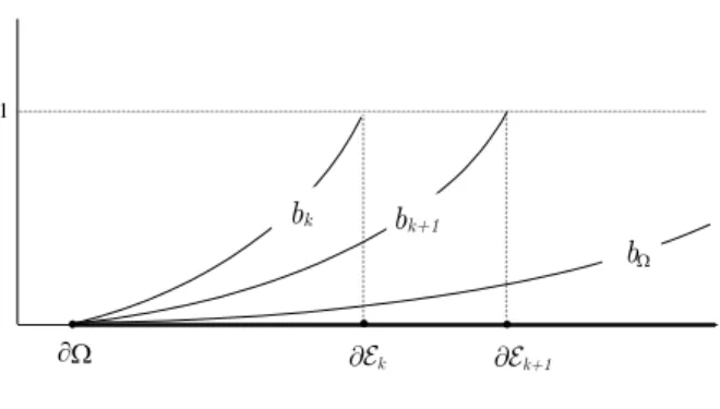
Definition 4.2. The subharmonic potential bΩof an open set Ω is the supremum of all admissible subharmonic functionsvfor Ω such thatv≤1.The superharmonic potential sΩof Ω is the infimum of all admissible superharmonic functions for Ω.
If there is no admissible subharmonic (superharmonic) function, then we natu-rally letbΩ≡0 (respectively,sΩ≡1). It is obvious that always
sΩ+bΩ= 1,
and the function bΩ is increasing on expansion of Ω whereas sΩ is decreasing. Clearly, Ω is massive if and only ifbΩ6≡0 andsΩ6≡1.
The function bΩ is called also the harmonic measure of the set F := M \Ω. Another term for sΩ is the reduced (or reduit) function of F. Let us emphasize that the functionsbΩ,sΩ are determined by the set Ω intrinsically.
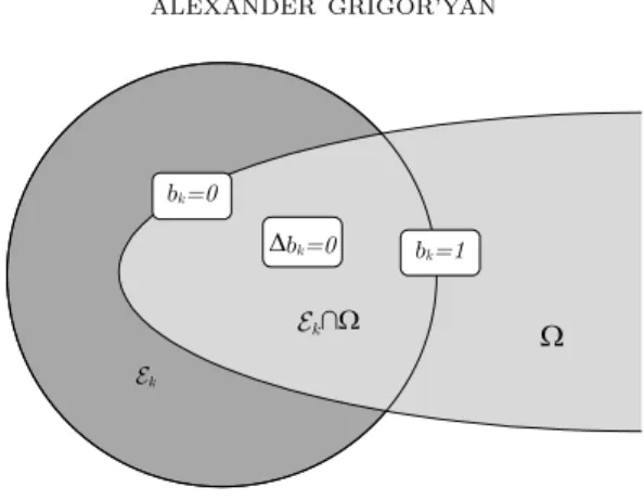
For a set Ω with smooth boundary, we will constructbΩandsΩas the limits of solutions of a series of certain Dirichlet problems. Choose an exhaustion{Ek}ofM so that the boundaries∂Ek and∂Ω are transversal, and solve, for any set Ω∩ Ek,
Figure 10. Functionbk
the following Dirichlet problem (see Figure 10)
∆bk= 0
bk|∂Ω∩Ek= 0
bk|∂Ek∩Ω= 1.
(4.27)
Proposition 4.3. Let Ω⊂M be a non-empty open set. (i) Assume thatΩ has non-empty smooth boundary. Then
bΩ= lim
k→∞bk in Ω.
The function bΩ is continuous, subharmonic onM and harmonic in Ω. Re-spectively, the functionsΩis continuous, superharmonic onM and harmonic inΩ.
(ii) For any proper open setΩ, we have bΩ= sup
Ω0 bΩ0,
where the supremum is taken over all regionsΩ0with smooth boundaries whose closure is contained in Ω.
(iii) The following dichotomy takes place:
either Ωis non-massive,bΩ≡0and sΩ= 1 orΩ is massive,supbΩ= 1andinfsΩ= 0.
Proof. (i) By the maximum principle, the sequence {bk} is decreasing. The limit b∞:= limk→∞bk is harmonic in Ω, continuous up to∂Ω and vanishes on∂Ω.Let
us extend b∞ by setting it equal to 0 in M\Ω. We claim thatb∞ =bΩ. Indeed, the function b∞ is obviously a continuous subharmonic function, 0≤b∞≤1, and b∞ vanishes outside Ω. If there is another functionv possessing these properties, then by the maximum principle, v ≤bk in Ek∩Ω, whencev ≤b∞. Hence, b∞ is
the supremum of all admissible subharmonic functionsv such thatv≤1, that is, b∞=bΩ (see Figure 11).
Note that if∂Ω is not smooth, thenb∞may be discontinuous at irregular points of the boundary∂Ω.
(ii)SincebΩ≥bΩ0, we have only to show that bΩ≤sup
Ω0 bΩ
1
Figure 11. Sequence of bk
For any open Ω0 such that Ω0 ⊂ Ω , there exists an open set Ω00 with smooth boundary such that Ω0 ⊂Ω00 and Ω00⊂Ω, whence bΩ0 ≤bΩ00.Therefore, it suffices to prove (4.28) without the requirement that∂Ω0is smooth. Letvbe any admissible subharmonic function for Ω. Take any ε ∈ (0,supv) and consider the set Ω0 =
{v > ε}. Since (v−ε)+ is an admissible subharmonic function for Ω0, we have (v−ε)+≤bΩ0.
By taking sup overv andε, we obtain (4.28).
(iii) By definition, bΩ 6≡0 is equivalent to the massiveness of Ω. Let us show that bΩ 6≡ 0 implies supbΩ = 1. If supbΩ =: c < 1 then, for any admissible subharmonic functionv, we have supv≤c.However, then the functionc−1vis also admissible subharmonic, whence, by the definition ofbΩ, we obtainc−1v≤bΩand supbΩ≥1.
Example 4.6. Let us show that a half-space Ω in Rd is non-massive. Consider the
function uwhich is equal tobΩon Ω and is extended oddly over the boundary∂Ω to the whole space. Sinceuis harmonic inRd and bounded, the Liouville theorem
impliesu≡const and, hence,u≡0.Therefore,bΩ≡0, and Ω is non-massive. 4.5. Hitting probabilities. In this section, we compute, in terms of the function sΩ, the following probabilities.
1. The Px-probability that the Brownian motion Xt visits a set F ⊂M ever.
Denote it by
eF(x) :=Px{∃t≥0 such that Xt∈F}.
In the potential-theoretic language, the functioneF is called the reduit
func-tion ofF and is denoted by R1F.
2. The Px-probability that the Brownian motion Xt hits F at a sequence of
arbitrarily large times. Denote it by
hF(x) :=Px{∃ {tk} such that tk→ ∞andXtk ∈F, for all k∈N}.
Proposition 4.4. LetΩ⊂M be a non-empty open set with smooth boundary, and denote F :=M \Ω.
(i) (G.A.Hunt) For anyx∈M, we have eF(x) =sΩ(x).
Figure 12. The hitting probabilities eF andhF
(ii) Let us denote
P∞sΩ:= lim
t→∞PtsΩ(x). (4.29)
Then, for anyx∈M,
hF(x) =P∞sΩ(x).
Remark. The function bΩ(x) is also called the escape function of Ω because, due to (i), bΩ(x) = 1−eF(x) which is equal to the Px-probability of Xt escaping to
infinity within Ω, without touching∂Ω.4
Remark. The functionu:=P∞sΩis harmonic onM becausePtu=u. Thus,hF(x)
is a harmonic function ofxon all ofM. Let us recall for comparison thateF =sΩ
is harmonic in Ω but is superharmonic inM (see Figure 12).
Remark. Assertion (i) implies that massiveness has the following probabilistic meaning: the set Ω is massive if and only ifeF(x)6≡1.
Proof. (i)Ifx∈F theneF(x) = 1 =sΩ(x), and there is nothing to prove.
Now letx∈Ω.Choose an exhaustion sequence{Ek}, and consider the eventAk that the trajectory Xt hits the boundary ∂Ω before ∂Ek (see Figure 13). Clearly,
the sequence of events {Ak}is expanding, and their union is the event to hit ∂Ω (and thusF) ever, whence
eF(x) = lim
k→∞Px(Ak). (4.30)
On the other hand, letfk be a function on∂(Ek∩Ω) which is equal to 1 on∂Ω
and 0 on∂Ek, and letτ denote the first hitting time of∂Ω. We have
Px(Ak) =Ex(fk(Xτ)) =sk(x) (4.31)
wheresk solves the Dirichlet problem inEk∩Ω :
∆sk = 0
sk|∂Ω= 1 sk|∂Ek= 0.
(4.32)
4One should distinguish the following two events: (1) to never hit F, which has the P
x
-probabilitybΩ; (2) to stay in Ω for allt≥0, which has thePx-probabilityP∞Ω1≤bΩ.The latter may be strictly smaller than the former in the case when the process can reach infinity from within Ω in a finite time. If the manifoldM is stochasically complete, then we do havePΩ
F
k
x
k
k+1
Figure 13. EventsAk andAk+1
SincesΩ= limk→∞skby Proposition 4.3, we conclude from (4.30) and (4.31) that
sΩ=eF.
(ii)Denote byBt the event thatXT hits F at some time T ≥t. Then we have
the following identity
Px(Bt) =PtsΩ(x) =
Z M
p(t, x, y)sΩ(y)dµ(y). (4.33) Indeed, at time t, the Px-law of the Brownian particle y = Xt is p(t, x, y)dµ(y).
Since the Py-probability of the Brownian motion hitting F is equal to sΩ(y), we
obtain (4.33) by the Markov property.
Obviously, the sequence of events {Bt} is decreasing in t (which implies, in particular, that the limit (4.29) exists), and their intersection is the eventB∞ that the Brownian motion visitsF at a sequence of arbitrarily large times. Therefore,
hF(x) =Px(B∞) = lim
t→∞Px(Bt) =P∞sΩ,
which was to be proved.
4.6. Exterior of a compact. If Ω is an exterior of a compactFonM, then some additional criteria of massiveness of Ω hold true.
Proposition 4.5. Let Ω ⊂ M be an open set with non-empty smooth boundary and letF :=M\Ωbe compact.
(a) The following dichotomy takes place:
either Ωis not massive, sΩ≡1 andP∞sΩ≡1, orΩ is massive,sΩ6≡1 andP∞sΩ= 0. (b) We have
Z ∂Ω
∂sΩ ∂ν dµ
0= cap(F), (4.34)
whereν is the outward normal vector field at ∂Ω, and
Z M
|∇sΩ|2dµ= cap(F). (4.35) Corollary 4.6. Let Ω⊂M be an open set with non-empty smooth boundary and letF :=M\Ωbe compact. Then