The Lane Regional Air Pollution Authority (LRAPA, Springfield,
OR) and the Environmental Protection Agency jointly developed a compact, portable, battery operated, air sampler for characterizing respirable dust (PM,o) , lead or carbon monoxide (CO) in an airshed.
The sampler (LRAPA Portable Sampler, Model 3.1) can monitor in
airsheds where permanent sites are not practical in order to
estimate the community pollutant exposure and to determine the
spatial and temporal variation of pollutant levels.
The decision regarding where to locate these samplers in an
airshed is often based on subjective considerations. Nontechnical
factors, such as convenience and accessibility, may dominate the
selection of a specific monitor site within a study area. A
guidance protocol was developed which quantitatively establishes
the portable monitor locations based on dispersion modeling and
statistical analysis.
A field study performed in Weehawken, NJ characterized the
ambient PMiq concentrations in the vicinity of the Lincoln Tunnel
entrance using the LRAPA sampler. Monitors were located based on
the guidance protocol at twelve separate locations within a 2 km X
2 km square grid surrounding the tunnel entrance. Three of these
sites contained collocated samplers. Results indicate the siting
model performed well, yielding a positive correlation between the
model's predicted concentration rank at each site and the actual
rank experienced in the field. A calculation of Kendall's
model performed best on clear, moderately windy days while less accurate results appeared on days with large fluctuations in wind direction. In addition, the model tended to underpredict the effects of auto emissions on the urban area's total aerosol concentration. The information obtained from the samplers provided a complete depiction of the PM,o concentration distribution
throughout the study area. Monitor collocation data demonstrates
that the LRAPA samplers provided consistent pollutant concentration
measurements with over 90% of the concentration readings yielding
1.0 Introduction ... 1
2.0 Background... 4
3.0 Network Design Methodology ... 7
3.1 Preliminary Information ... 7
3.2 Concentration Estimates ... 9
3.2.1 Model Algorithms ... 9
3.2.2 Performance Characteristics of the ISCST2 Model... 13
3.3 Selection of Monitor Sites ... 16
3.3.1 Meteorological Data Input... 16
3.3.2 Initial Selection ... 16
3.3.3 Final Site Selection... 19
3.4 Computer Program ... 20
4.0 Network Design Application - Weehawken, NJ Study .... 21
4.1 Establishment of the Study Area... 21
4.2 Dispersion Modeling ... 24
4.2.1 Source/Emissions Information ... 24
4.2.1.1 Point Sources ... 24
4.2.1.2 Volume Sources ... 25
4.2.1.3 Area Sources... 31
4.2.1.4 General Considerations ... 31
4.2.2 Meteorology... 31
4.2.3 Topography... 3 3 4.2.4 Special Model Requirements ... 33
4.3 Location Evaluation ... 34
4.3.1 Receptor Rankings ... 34
4.3.2 Location Determination ... 34
5.0 Field Study Results ... 36
5.1 Introduction... 36
5.2 Study Objectives ... 37
5.3 Final Site Selection... 38
5.4 Concentration Results ... 38
5.5 Data Quality... 40
5.5.1 Sample Collection ... 40
5.5.2 Analytical Precision ... 41
5.5.3 Monitor Performance ... 43
5.5.3.1 Study Design ... 4 3 5.5.3.2 Study Results ... 45
5.6 Analysis of Model Performance ... 49
6.0 Conclusions... 63
6.1 Model Performance ... 63
6.2 LRAPA Sampler Performance ... 66
6.3 Field Study Results ... 67
APPENDIX A - Concentration Isopleths ... 69
APPENDIX B - Field Study Data... 81
APPENDIX C - ISCST2 Input File... 91
APPENDIX D - The SITE Computer Model... 101
APPENDIX E - Meteorological Data... 108
APPENDIX F - Standard Operating Procedure for Field Study . . 117
FIGURE 3-1
FIGURE 3-2
FIGURE 4-1 FIGURE 4-2 FIGURE 4-3
FIGURE 5-1
FIGURE 5-2
FIGURE 5-3
FIGURE 5-4
FIGURE 5-5 FIGURE 5-6 FIGURE 5-7 FIGURE 5-8 FIGURE 5-9
GIS Map of Hudson County, NJ... 8
Gaussian distribution coordinate system .... 11
Topographic Map of Weehawken, NJ... 22
Standards for the Lincoln Tunnel Entrance ... 30
Final Site Locations... 35
LRAPA Monitor Collocation - Site 2... 47
LRAPA Monitor Collocation - Site 3... 47
LRAPA Monitor Collocation - Site 7... 48
Comparison of PM,o concentration readings from
LRAPA monitors and reference high-volume
samplers... 49SITE model comparison... 50
ISCST2 model comparison... 58
Constant wind direction comparison... 61
Comparison of hazy conditions... 62
Comparison of rain days... 62
APPENDIX A APPENDIX E
Concentration Isopleths for Weehawken, NJ Windroses for Newark, NJ Airport ...
70
LIST OF TABLES
TABLE 31 TABLE 41 -TABLE 5-1 TABLE 5-2 TABLE 5-3 TABLE 5-4 TABLE 5-5 TABLE 5-6 TABLE 5-7
TABLE 5-8
TABLE 5-9
APPENDIX B
-WIND PROFILE EXPONENT, p, USED BY THE ISCST2
MODEL... 12
MAJOR ROADWAYS ANALYZED IN HUDSON CO., NJ . . . . 23
MONITOR SITE DESCRIPTIONS ... 39
FIELD SAMPLING ERRORS... 41
BLANK FILTER ANALYSIS... 42
MONITOR EVALUATION (at EPA Facilities) ... 46
CONCENTRATION READINGS FROM THE NAAQS PERMANENT . 48 CONCENTRATION RANKS BASED ON FIELD RESULTS ... 54
KENDALL RANK CORRELATION COEFFICIENT CALCULATION (all sites) ... 55
KENDALL RANK CORRELATION COEFFICIENT CALCULATION (site number 9 omitted) ... 56
CONCENTRATION RANKS BASED ON MODEL RESULTS ... 60
ATM = Model averaging time (minutes)
C^ = average pollutant concentration at receptor, x
Cjj = pollutant concentration at receptor, x, for
meteorological condition, i
C,yg = average pollutant concentration (mass/volume)
Cj = pollutant concentration for meteorological condition, 1 (mass/volume)
H = Effective plume height
h„f = Wind speed anemometer height
h, = Stack height
K = Kendall correlation statistic
n = number of samples
n^ = number of concordant pairs of data
nj = number of discordant pairs of data
Q = Pollutant emission rate (mass/time)
p = Wind profile exponent
Pmti ~ probability of meteorological condition, i r = Pearson correlation coefficient
TR = residence time
u„f = Wind speed at anemometer height
u, = Wind speed at stack height
W = road width
CTy = lateral dispersion parameter (distance)
a^ = vertical dispersion parameter (distance)Oyg = initial lateral dispersion parameter (distance)
a^ = initial vertical dispersion parameter (distance)
1.0 Introduction
The Lane Regional Air Pollution Authority (LRAPA) and the
Environmental Protection Agency developed a compact, portable,
battery operated, air sampler for characterizing respirable dust
(PM,o) , lead or carbon monoxide (CO) in an airshed. The sampler
(LRAPA Portable Sampler, Model 3.1, LRAPA, Springfield, OR) can
monitor in airsheds where permanent sites are not practical in
order to estimate the community pollutant exposure and to determine
the spatial and temporal variation of pollutant levels.
The decision on where to locate these monitors is frequently
based on subjective considerations and personnel judgement. Nontechnical factors, such as availability, convenience and accessibility, often influence the selection of a specific monitor site within an area of interest. Recently, a study performed in Asheville, N.C. to determine the effects of woodstove emissions on the air quality of the region utilized the LRAPA sampler. According to Berg (1990), monitor sites were located based on local agency experience using information from topographic maps of the area, housing densities, traffic counts on the local roads, and emissions inventories. Another study done in Weirton, W.V. used
the LRAPA sampler to determine if additional permanent PMjo
monitoring stations were needed in the vicinity of a large steel
plant, and where these new NAAQS stations should be located (Erdman
et al 1990). For this project, the authors determined the
points of the steel mill and the topography of the surroundings.
A study done in El Paso, TX to determine the representativeness of
the existing NAAQS monitoring site placed the monitors in a gridded
pattern stretching along the U.S./Mexican border (Kemp 1992). No
studies characterizing pollutant concentrations on a neighborhood scale or smaller were found which established monitor locations by
a quantitative method.
This research project concentrates on developing an air
monitoring network for single airshed studies such that the
probability of locating the point of highest average concentration
experienced within a study area is maximized. This information is
important in either locating or relocating NAAQS monitoring
stations to adequately describe the air quality of the area,
confirming the location of an existing NAAQS monitoring station, or
to determine if an air quality problem even exists. Other possible
uses of portable air samplers which may require special
considerations for sampler siting are field validation tests for
air pollution dispersion models or special needs of the local
monitoring agency, particularly remote monitoring where electrical
power is not available.
The siting methodology proposed in this document for improving
and standardizing sampler siting incorporates the use of dispersion modeling and statistical analysis. One of the problems this
project hopes to solve is the required or desired spacing between
the individual monitor sites in order to adequately describe the
3 preliminary monitor siting is available through the United States
Environmental Protection Agency (EPA), and can be obtained in a
reasonable period of time. Section 3.0 provides further
4
2.0 Background
General information on air quality monitoring can be found in
several books, as well as some EPA documents covering the topic.
One of the first books to adequately describe the subject was
Stern's Air Pollution (1976) which has a section devoted to ambient
air quality surveillance. This section lists the three major
categories of effects on air pollutants that must be considered,
which include 1) source influences, 2) demographic influences, and
3) meteorological influences. The author also suggests a variety
of information needed to develop a good siting plan, including the
region's stationary sources, mobile sources, population
distributions, meteorology, topography, land use, etc.. Stern
illustrates the limitations associated with air quality monitoring
by declaring that no sampling or monitoring system can represent
all the variability that exists in ambient air quality because of
the atmosphere's dynamic nature. Other books which contain similar
information on air quality monitoring include Noll and Miller
(1977), Benarie (1980), and Godish (1991). Many EPA documents and
training manuals give insight on some monitoring studies done in
the past as well as some design criteria for air sampling networks.
Ludwig et al. (1977) and Koch et al. (1984 and 1987) state many of
the criteria required for siting monitors, while training manuals by Bowman et al. (1988) and Wilson et al. (1983) also provide
similar information. These methods provide qualitative means of
establishing the locations of monitors in an air quality
5
The model used for this project is based on the concept
developed by Lui, et al. (1986), which establishes a potential
monitor's "sphere of influence" (SOI) based on statistical analysis
of expected pollutant concentrations obtained from a pollutant
dispersion model. The premise of the model is that the optimum
number and location of monitor stations can be established by
estimating the probability of recording the maximum concentrations
at a given station location and omitting those locations which
provide redundant data. The method used to establish this optimal network incorporates the use of a dispersion model to determine potential pollutant concentrations for an area under various conditions. Once the model estimates the region's pollutant
concentration patterns for various conditions, this concentration
pattern is statistically analyzed to determine the best sites for
monitor placement based on the probability of occurrence. This
occurs by entering the assorted meteorological conditions and emissions factors and quantifying the possibility of each event occurring, resulting in a ranking of each potential monitor
location. The model then determines the SOI for each monitor
location by calculating a correlation coefficient between each grid
point in the region of interest. A predetermined value for the
correlation coefficient determines the other grid points included
in a particular grids SOI.
other similar approaches to siting air monitors can be found
in the literature. Hougland (1976, 1977 and 1980) presented one of
located monitor sites based on maximizing coverage factors, such as strength of emission source, distance from the source and local meteorology, for each source in a study. Husain and Khan (1983) developed a methodology using Fisher's information measure to
determine the optimum number and location of monitors in a network.
This technique utilizes a statistical relationship developed by
Fisher (1966) for estimating the information content in a set of
data. Noll and Mitsutome (1983) developed another method which
establishes monitor locations based on expected ambient pollutant
dosage. This method ranks potential locations by calculating the
ratio of a station's expected dosage over the study area's total dosage. A more complex methodology developed by Nakamori and
Sawaragi (1983) determines the representative areas of monitor stations in urban areas. The method enables the participation of specialists to take into account unique economic and physical conditions present in the study area. A similar procedure was developed by Kainuma, et al. (1990) which evaluates several types of siting objectives and performs a multiattribute utility function method to determine the optimal locations. All of the
methodologies evaluated used urban or regional scale studies. No
3.0 Network Design Methodology 3.1 Preliminary Information
Once the neighborhood scale study area for an air quality
investigation is chosen, a map of this area can be made through
EPA's Geographic Information System (GIS) which contains population
densities, pollutant source locations, and almost any other type of
geographical information necessary for a particular study. Also,
a receptor network can be superimposed onto this map to facilitate
use with a dispersion model. 100 meter X 100 meter grids comprise
the entire receptor network. This grid size is chosen as a
compromise between detailed siting and possible restrictions
located within the grid. For larger grid sizes, the siting
guidance would be much less valuable because of the large number of
possible locations for siting, and the higher probability of
variations of pollutant concentrations within the grid. Smaller
grid sizes create a strong possibility that no adequate sites can
be found within the grid. Thus, the grid size chosen allows a
precise portion of the study area to be chosen for a site, yet
allows enough flexibility for determining the final monitor
location. Figure 3-1 illustrates the receptor grid chosen for the
Weehawken, NJ study. Detailed maps of the area's topography and
road systems (at 1:24000 scale) can also be purchased from the
United States Geological Surveys (USGS) Department.
Information regarding pollutant emissions from industries
located in the study area can be obtained through EPA's Aeromatic
HUDSON CO., NJ
PopulottoR Donsdy
(peopie per squore kliometer)
No P»oplt or Ofltildt ef Viuiitt Ctttnty 0 U 5,000 ^mn 25,000 to 30.
! 30,000 te 3M0O "im 35.000 U 40.000 5.000 to tO.GOO
10.000 td 15,900 m
25.O00 U 20.000 ^^i 40,000 to SO.OOC
Hudson Co., N.J. figure 3-1
Popyioiion Density
(people per squore klfometer}
Mo PeopU or Catildc of Hh^sob Coirtty
D to 5,000 mrm 25.CO0 to 30.000
5,000 to 10,030 i i 30.000 to 35,000
'.0,000 to 15,000 r-.:^-:"q JS.COO tc 40,600
15,000 to 20.000 fefifr^ 40,000 to S0,O0C
2C,CO0 to 25.800 ^HB 50,000 t» 75.
source location, stack height and diameter, and gas temperature and
exit velocity.
Next, the region's traffic data can be acquired from the
individual state's Department of Transportation as well as the
region's County Engineering Department if the County maintains its own roadway system. This data consists of the average daily traffic (ADT) counts and the location where these counts were made. Additional information such as average travel speed and the percent of trucks using the facility is helpful, but not necessary.
Once this data is collected, pollutant emission factors for the vehicles can be estimated based on the guidelines established
in AP-42 (USEPA, 1985a). USEPA (1991) provides some updated procedures for specifically preparing PMiq emissions inventories.
The PART computer model developed by Energy and Environmental
Analysis, Inc. (USEPA 1985a) can be used to estimate vehicle particulate emissions. This data is entered into a pollutant
dispersion model to determine the expected pollutant concentrations
within the area of interest.
3.2 Concentration Estimates
3.2.1 Model Algorithms
The Industrial Source Complex Short Term (ISCST2') dispersion
model calculates the potential pollutant concentrations expected within the study area. This is a steady state Gaussian plume model
10 that can assess pollutant concentrations from a wide variety of
sources in either rural or urban areas (USEPA, 1986) . It is one of
the most widely used programs within the EPA modeling community because of the many options available to the user. The model
processes hourly meteorological data, and estimates the pollutant
concentrations based on each hour of input meteorology for each
receptor.
For the analysis of a point source (such as a stack) , the
model uses the steady state Gaussian plume equation for a continuous elevated source. The origin is placed at the base of
the source with the x-axis corresponding to the wind direction, the
y-axis corresponding to the normal crosswind direction, and the z-axis representing the vertical direction (see Fig. 3-2). The
hourly pollutant concentration at a downwind distance of x meters
from the source, a crosswind distance of y meters and an elevation of z meters is given by:
C{x,y,z,K) = Q
2KU^OyO^
exp 2al
exp
^ {z-H)^^
2a'
+exp
^ (z+H)^^
2o1 /J (1)
where: Q = pollutant emission rate (Mass/Time) u, = mean wind speed at release height H = effective plume height
Oy = lateral dispersion parameter
since most wind speed data is specified only at the anemometer
height, the wind power law estimates the wind speed at the release
height. This equation is given by the following:
(2)
where: u„f = observed wind speed
href ~ anemometer height
h, = stack (or release) height
p = wind profile exponent
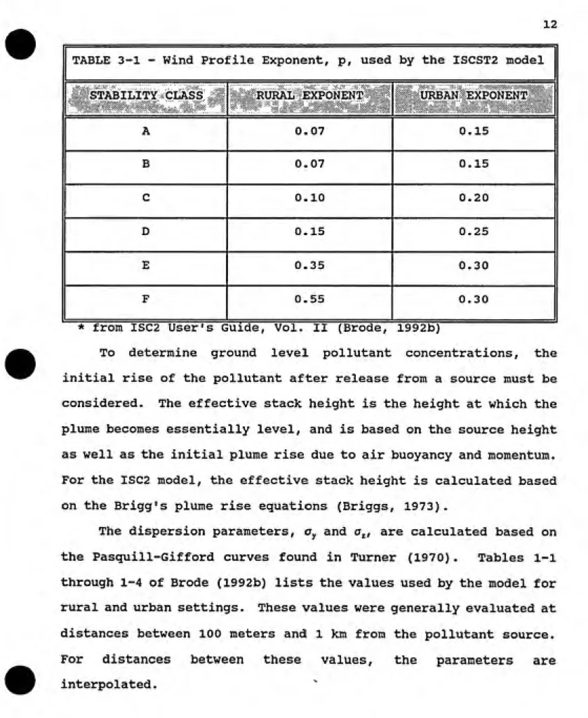
Values for p are a function of stability class and wind speed, and
may be provided by the user where site specific meteorological
information is available. For details on calculating p, Arya
(1988) should be consulted. Table 3-1 lists the default values
used by the ISCST2 model.
(x,-y^)
(i.-y,o)
12
TABLE 3-1 - Wind Profile Exponent, p, used by the ISCST2 model
STABILITY CLASS RURAL EXPONENT URBAN EXPONENT
A 0.07 0.15
B 0.07 0.15
C 0.10 0.20
D 0.15 0.25
E 0.35 0.30
F 0.55 0.30
* from ISC2 User's Guide, Vol. II (Brode, 1992b)
To determine ground level pollutant concentrations, the initial rise of the pollutant after release from a source must be
considered. The effective stack height is the height at which the
plume becomes essentially level, and is based on the source height
as well as the initial plume rise due to air buoyancy and momentum. For the ISC2 model, the effective stack height is calculated based on the Brigg's plume rise equations (Briggs, 1973).
The dispersion parameters, a^ and a^, are calculated based on
the Pasquill-Gifford curves found in Turner (1970). Tables 1-1
through 1-4 of Brode (1992b) lists the values used by the model for rural and urban settings. These values were generally evaluated at
distances between 100 meters and 1 km from the pollutant source.
For distances between these values, the parameters are
The ISCST2 model calculates volume sources by dividing the
region into a finite number of point sources. Therefore, the
Gaussian equation can also calculate concentrations resulting from
volume sources. The lateral dispersion parameter is based on the
distance between the sources while the vertical dispersion
parameter is based on an empirical formula developed by the
California Department of Transportation (Benson, 1979) . Details of
the vertical dispersion parameter are discussed in Section 4.2.1.2.
Area source concentration calculations use an equation which
represents the region as a finite crosswind line source.
Therefore, the methodology used for this calculation is similar to the calculation for a volume source. For further information on any of the algorithms used by the model, Erode (1992b) should be consulted.
After the ISCST2 model generates the concentration estimates,
the results can be written into an output file using the POSTFILE
command in the model's OUTPUT pathway. This file becomes the input file for the computer program developed to determine the monitor sites. Section 3.3 and Appendix B discuss the details of this
program.
3.2.2 Performance Characteristics of the ISCST2 Model
In general, dispersion models based on the gaussian
approximation tend to have a factor of two accuracy in calculating
pollutant concentrations (AMS, 1978). For this project, the
14
relative precision of the predictions is essential. The model must
accurately predict the relative spatial and temporal variations of the pollutant over the study region at distances of 100 meters or less. Thus, situations where the model tends to underpredict or
overpredict concentrations in relation to spatial and temporal
changes in the input data must be known.
According to Schulman, et al. (1981), large overpredictions
tended to occur at the lowest wind speeds while the largest
underpredictions occurred at high wind speeds. In addition, the study found that the model tended to underpredict pollutant concentrations from low-level sources. One reason may be that the model overestimates plume rise for these low-level sources because of the manner in which wind speed is calculated. The method used
by the model assumes wind speed increases with height only up to
the stack height (see equation 2), with the wind speed above this
height constant. If wind speed continues to increase vertically
above the stack height, the model may overestimate plume rise due
to buoyancy and consequently underestimate the contribution of these sources to the overall concentrations. This characteristic
could cause the model to significantly underestimate the effect of
the pollutant at receptors located near the source. Studies by
Bowers and Anderson (1981a and 1981b) verified the model
underpredicted pollutant concentrations at receptors located near
the source but did not specify if the source emission heights were
near groundlevel. Turner (1970) stated that models incorporating
from low-level sources in urban areas because the dispersion parameters were developed for rural areas. Since increased surface
roughness and air buoyancy (due to the heat island effect) tend to
create more mixing effects in urban regions, there should be
increased dispersion in these areas. This model characteristic
could overpredict pollutant concentrations at some receptors and
underpredict the concentrations at other receptors depending on
source locations and meteorological conditions.
Londergan, et al. (1981) found that proper stability class identification affects the accuracy of the model's prediction. The coefficients associated with stability class, along with the wind
speed and direction, are important in predicting plume behavior.
This effect tended to be more important for estimating the actual
concentration values, not the spatial variations of the pollutant.
Al-Sudairawi and MacKay (1988) established the effect of
meteorological input data accuracy on the performance of the ISCST2
model. As expected, this study found that meteorological input
data must be representative of the actual conditions at the region
being modeled for accurate predictions to occur.
The ISCST2 model does not account for physical and chemical
processes which may alter the size and distribution of airborne
particles. Factors such as particle agglomeration or
16
3.3 Selection of Monitor Sites
3.3.1 Meteorological Data Input
Meteorological data is entered into the ISCST2 model based on the various combinations of meteorological conditions experienced
at the weather station, not on the daily conditions seen at the
site. Thus, each hour of meteorological input data represents a specific combination of wind speed, wind direction and stability class, and is unrelated to the specific conditions experienced on a given day. The model calculates the pollutant concentrations at each receptor for the given combination of meteorological
conditions. The average concentration expected at each receptor,
C^, for n meteorological conditions can then be calculated by:
^av^ = Efi *^--t,) <3>
1=1where C,. represents the concentration expected for meteorological
condition i, and p^, is the probability of meteorological condition
i. Thus, the average concentration at each receptor is the sum of
the expected pollutant concentration for each combination of
meteorological conditions multiplied by the probability of
experiencing that given combination based on historical
meteorological data.
3.3.2 Initial Selection
Once the pollutant concentrations are determined for the given
identified and ranked based on the expected average pollutant
concentration at each site. Each receptor site in the receptor grid is classified as a potential monitor site. As described above, the average concentration at each receptor site is calculated based on the probability of occurrence of each specific meteorological condition. Thus, the receptor sites with the greatest probability of experiencing the highest pollutant concentrations can be identified. Each location is ranked from
highest to lowest concentration.
After ranking the potential monitor sites, the representativeness of the air quality data from that monitor for an area surrounding the site is calculated based on the previously mentioned analysis by Liu et al. (1986). This model determines a monitor's "sphere of influence" (SOI) which is defined as the area over which the air quality data for a given station can be considered to be representative, or extrapolated with known
confidence.
In order to determine a site's SOI, the model utilizes the covariance structure of the concentrations. Pearson's correlation
coefficient, r, is calculated between values of pollutant
concentration at a given site and the corresponding values at
neighboring sites. For a site located at receptor a being compared
to a site located at receptor b for n meteorological conditions,
18
•
E (C-ai-Ca) (C^i-C^)
i=i
r = , ^ = (4)
N
i=l Wwhere
^= ^-^
E^-i
(5)n
and
E^^i
(6)n
which represent the average concentrations experienced at the sites
during the time period analyzed.
Assuming C, and C^ are random variables from a normal
distribution, a probability distribution for a correlation
coefficient, r, associated with a sample size, n, randomly drawn from an infinite population with a true correlation coefficient, p, can be derived. This probability distribution, p, is defined as:
P(r|n,p) - [^rfi;-;- (l-r^) '--'/^ ^/^" ^ arccos (-pr) ^^^
1^(^-3)! d(pr)"-2 ^i-(pi)2
To determine the confidence level of the hypothesis that r=p„ with
E =fpir\n,pj dr (8)
Therefore, assuming a linear relationship between the variables, the square of the correlation coefficient explains the fraction of
the variance of C^ that can be explained by the variation in C,.
Thus, a monitor site's SOI comprises those neighboring sites whose
variance can be explained by the original site's variance within a
certain degree of confidence.
Using this procedure, the SOI for the highest ranked monitor
site can be calculated. In order to determine the second monitor
site, the SOI for the second highest ranking receptor site is
analyzed. If this site is located within the SOI of the higher ranking site, it will not be considered as a monitor site. If this
condition is not met, the site is chosen as a monitor location. This procedure continues with each receptor site in descending
order of average concentration until all the monitor sites available for the study are determined.
The monitor network's percent coverage, which can be used to
estimate the network's representativeness, consists of the total number of receptor grids included within the combined SOI's divided by the total number of grids in the study region.
3.3.3 Final site Selection
20
study area. Whenever possible, this site should conform to the
guidelines for air quality monitoring established in the Code of
Federal Regulations (40 CFR Part 58).
Since the LRAPA monitors are designed to mount on telephone
poles (see LRAPA, 1992), most of the sites will be near roadways. After classifying a grid site as a monitor location, the roadway which experiences the highest traffic volume within that grid site is identified. The monitor should be located on a pole along this
roadway as near to the center of the grid as possible. If a
suitable site cannot be located within the selected grid, a site found inside the neighboring grid with the highest correlation coefficient with the originally selected grid will be chosen. Grids are analyzed in descending order until an acceptable monitor
site can be located. If a roadway is not located within a chosen
grid, the first acceptable location closest to the center of the grid is chosen.
3.4 Computer Program
A computer program called SITE was developed for this project to assist with establishing monitor locations for sampling studies incorporating the siting methodology described above. To run this
program, an output file from the ISCST2 dispersion model must be
generated. Further information on how to use this program, as well
4.0 Network Design Application - Weehawken, NJ Study
4.1 Establishment of the Study Area
Figure 3-1 shows a map of the study region including
population densities, some pollutant point source locations and the
receptor grid chosen for the study. Fig. 4-1 includes the
topography of the region as well as the roadway network in the
area. The study region includes the towns of Weehawken, Union
City, and North Bergen (all located in Hudson County, NJ).
Additional pollutant sources evaluated for the study are located in other parts of Hudson County, Bergen County, NJ and New York
County, NY. The precise area of interest specified for evaluation
is an approximately 2 km X 2 km square area encompassing portions
of Weehawken, Union City, and North Bergen. Major roadway features
in this area include the entrance for the Lincoln Tunnel and
Interstate 495. Table 4-1 lists the roads, along with ADT values,
analyzed in this study.
The 100 meter X 100 meter grids included in the study area
(shown in Figure 3-1) represent the potential monitor sites. A
receptor point located in the center of each grid depicts the
concentration values obtained from dispersion modeling that
ͣ
»iM« m c^wMvi ͣilK No T«n Btonvtm •> Trimmmiaii
timm iwnMi.ii mm i» « ͣ nv ͣ« mm MV ?<I.
ͣͣ
X4IIM4 1fc« II ͣ ^ « 11— fc Mi^MMt »»^Mi
ͣ
OW C(>SS«CM«n
r^ Mu. ͣͣ"ͣ !•.
Hw<t«|i«
ͣͣ
»«' Xlt ^^—^ l»aiwMf...
• l«>«»i»»»-wiim »>
WEEHAWKEN. N J-N. Y
ͣ
IMtiM I M-MMCI TCM
iS
DtnPt
tckrnw Ik •<•
U A N H
It. LI
»infill
SCALE 174000
e I tKl
I lutOMnc*
CONTOU* INTeitVAL 10 rctT MnONM. atOMTlC VCRTICiU. OATUW OT IM«
KfTH eUlWn AND tOUNDINCS IM rCrt-OATUM n WUN low WATtK
TM( ltlAfO«»«l' KTWtCil THE TWO 0<^TW«t It «««l*llC
ͣ
nOMimt tMe«« nnitUMit tNl a^moiihau lwi d* Mmi migm «*n>
mt MM •AMCC e^ noc it vMMntAtciT«.: rtn m thi muoim *i»ti
AMD 1.1 rtn M TN( MACUNSACK MO MMAIC tl»C«i
IMS MAP cownjcs vrrM mational ma» accuracy stanoards
KM »ALE tY U. t. CIOLOGICAL SURVEY
eCMVEK. OOLOKAOO RZZi. OR RESTON. vmciNIA 22012
* fOUn CttCR—iO TBKXSIUrMC MAn AND BYMWU • AVAMMi ON KQUEST
FIGURE 4-1 - Topographic map of a portion of Hudson County, NJ including the
TABLE 4-1 ^Ira NORTH BERGEN NORTH BERGEN NORTH BERGEN NORTH BERGEN NORTH BERGEN NORTH BERGEN UNION CITY UNION CITY UNION CITY UNION CITY UNION CITY UNION CITY UNION CITY UNION CITY XJNION CITY WEEHAWKEN WEEHAWKEN WEEHAWKEN WEEHAWKEN ^M?/|jOCAyiOlir
TONNELLE AVE. - S. of Paterson Plank Rd. TONNELLE AVE. - N. of Paterson Plank Rd. J.F. KENNEDY BLVD. - S. of 1-495
J.F. KENNEDY BLVD. - N. of 1-495
PATERSON PLANK RD. - S. of Tonnelle Ave. PATERSON PLANK RD. - N. of Tonnelle Ave.
BERGENLINE AVE. - 32nd St. to 33rd St.
BERGENLINE AVE. - 31st St. to 32nd St.
BERGENLINE AVE. - 29th St. to 30th St.
32ND STREET - Central Ave. to Bergenline Ave.
32ND STREET - Bergenline Ave. to New York Ave.
31ST STREET - Central Ave. to Bergenline Ave.
31ST STREET - Bergenline Ave. to New York Ave.
30TH STREET - Central Ave. to Bergenline Ave.
30TH STREET - Bergenline Ave. to New
York Ave. BOULEVARD EAST
PARK AVE. - S. of Lincoln Tunnel WILLOW AVE. RAMP from 1-495
24
4.2 Dispersion Modeling
As discussed in Section 3.0 of this document, the study utilized the ISCST2 dispersion model. This model was chosen
because of its flexibility in analyzing a large variety of sources in an almost unlimited number of situations. Also, the model is
widely used and scrutinized by the EPA modeling community. As previously mentioned, a number of studies have been done identifying the model's performance over long and short distances.
Appendix B lists the ISCST2 input code used for the Weehawken study. As shown in the code, the urban mode plume dispersion
values were used, as well as default values of wind profile exponents and vertical potential temperature gradients. No downwash was calculated, and emission rates were assumed constant over the entire study period. The following sections describe the
special considerations applicable to the different types of
pollutant sources. The ISC2 User's Guide (Brode, 1992a) should be
consulted for further information about the source code.
4.2.1 Source/Emissions Information
4.2.1.1 Point Sources
Point sources were chosen and modeled based on information
obtained from the AIRS database. The ISCST2 model analyzed sources
located in Hudson and Bergen Counties in New Jersey, as well as New York County in New York City. The ISCST2 input file found in
Unfortunately, at the time of this study, AIRS reported
particulate data as total suspended particulate (TSP) for both New
Jersey and New York. To convert these values to a PMk, equivalent,
a conversion ratio of 0.485 (PMjo/TSP) was chosen based on the
studies by Rodes (1985) and Frank, et al. (1984). Although these
ratios are not site specific but were developed to convert TSP
pollutant concentrations to PMiq values at NAAQS monitoring sites,
the ratio was assumed to apply to the study area because of the
wide range of sources evaluated. Since most of these sources are
located outside the receptor area, the pollutants from all sources
should be well mixed and thus represent a typical urban airshed. EPA is currently updating the AIRS database to report particulate sources as PM,o, so this conversion should not be necessary in the future.
4.2.1.2 Volume Sources
All roadways were evaluated as volume sources for this analysis, and were divided into equivalent sections four times as
long as the road width. Although the ISCST2 user's guide
recommends that these segments only be twice the road width, the longer sections became necessary in order to limit the overall
number of sources to an amount the model could process. Thus, for
the determination of the initial horizontal dispersion parameter,
CTyo, the formula recommended in the guidance document was used:
AW
2.15
26 where W represents the road width (in meters) . This equation still provided uniform dispersion to receptors located close to the source. For the determination of the initial vertical dispersion
parameter, a^, the empirical formula developed by the California
Department of Transportation (CALTRANS) for the CALINE3 model was
used (Benson, 1979):
where ATIM is the model averaging time (60 minutes for this study)
and,
o^ = 1.8+0.11 (TR) (11)
with.
TR = — (12)
2u
where TR = residence time (sec) u, = wind speed (m/sec)
The residence time represents the period when the exhausted
pollutant remains in the mixing zone above the roadway. Thorough
mixing of the pollutant is assumed in this zone due to the buoyancy
and momentum of the exhaust gas and the wake effects from the
passing vehicles (Benson, 1979). For this analysis, the average
wind speed for the month of July (over the years 1985-1989) was
used to evaluate a^. Section 4.2.2 provides more detail on the
meteorological data.
County (NJ) Engineering Department provided this data. The
locations described represent the areas of traffic counts made in
the last 5 years, which gives a good indication of the heavily
traveled roads in the area. Counts for Interstate 495 were
unavailable from either source. The ADT's along 1-495 were
estimated based on the traffic at the Lincoln Tunnel tollbooths
subtracted by the number of vehicles exiting and entering via the
ramps at Park Ave., Willow Ave., and Boulevard East (the Mueller
ramp). These ramps are the only major access points within the
study area before the ramp for J.F. Kennedy Blvd on the western end of the study area.
Average speeds along each road are estimated based on the
roadway type. Light duty city streets are given an average speed of 25 mph because these streets tend to carry local traffic
travelling short distances. Heavy duty city streets usually
average speeds of 35 mph because these tend to carry transient
traffic, yet, within cities, the speed limits are rarely over 35
mph. Due to the high traffic volumes in this region, highways
average speeds of 55 mph.
Road widths are estimated based on the information from the
USGS map. 2-lane roads are assumed to average 10 meters (approx. 30 ft) in width while 4-lane roads are estimated at 15 meters.
Interstate 495 is evaluated based on an average of 6-lanes (or 30
meters) throughout the study area.
Calculations of emission rates along each street section used
28
particulate emissions from mobile sources based on the regulatory
guidance in AP-42 (USEPA, 1985a). The program also accounts for
particulate emanating from brake and tire wear. Since leaded fuel
is extremely uncommon, misfueling rates are set equal to zero,
leaving the lead content for both leaded and unleaded fuel at 0.014
g/gal. For further information on lead content. Table 2-2 of AP-42
should be consulted. Additional information on the calculation of
emission factors from mobile sources can be found in USEPA (1985b). The emission rates for all roadways evaluated in the study can be identified in the ISCST2 input code of Appendix B.
The Lincoln Tunnel and the surrounding toll booths presented a unique difficulty in modeling. To estimate the emissions from vehicles at the tolls, this section is modeled as an area source.
Average speed is assumed to be 5 mph beginning a distance of approximately 500 ft (150 meters) from the tollbooths. This average speed takes into account vehicle deceleration as cars approach the booths, and, more importantly, the starting and stopping which occurs as the vehicles queue at the booths. Since
the tolls are only located on the eastbound lanes (traffic entering New York City) , only this section was modeled as an area source
with an ADT of half the vehicles using the tunnel. The westbound
lanes were modeled similarly to the other roadways with an average
speed of 45 mph (as vehicles accelerate from the 35 mph speed limit
in the tunnel to the 55 mph speed limit on 1-495) and a width of 15
meters. The stretch of road between the tollbooths and the tunnel
estimated based on a speed of 35 mph. Figure 4-2a provides details of the road network in the vicinity of the Lincoln Tunnel entrance.
Based on information from the New York/New Jersey Port
Authority (Calo, 1992) , an assumption was made that 80% of the
vehicle exhaust emitted in the tunnel was removed through the
tunnel's ventilation system, while the remaining 20% escaped
through the entrance portals. Thus, 10% of the total exhaust
emitted inside the tunnel exits through the portal on the New Jersey side. The amount of pollutant emitted is based on the tunnel's length and the particulate emission factor for vehicles cruising at 35 mph. Figure 4-2b is a diagram detailing the design of the tunnel. No correction was made for particle settling or deposition inside the tunnel since a large majority of the particulate exiting through the portals is emitted only a short distance from the entrance. Pollutants exiting through the portals is assumed thoroughly mixed within a distance of 50 meters from the entrance by vehicle wake effects both inside and outside of the tunnel.
Train emissions were not considered for this study. Since the West Shore Terminal (located in northern Weehawken) is no longer used and the Conrail and Amtrak lines in the area are diverted
underground through this region, the only rail line in the study
area is a short section of the Susquehanna and Western line which
FIGURE 4-2a - Schematic of the Lincoln Tunnel Entrance. All
labeled roadways are residential and not under the
jurisdiction of the New York/New Jersey Port Authority.
H.D&
?
Linccin Tunnel Entrance In
Weetiawken,
NJ
r—»
FIGURE 4-2b - Design of a typical portal tube. As can be seen
in Figure b, the tunnel consists of three separate tubes: north/ central and south.
rtan m rut.
MM rm^t ͣ
«>-K#ri« TO •«<ͣ
Typical Pcrtal Crcss-Sectlcn fcr
4.2.1.3 Area Sources
There were no sources analyzed as area sources within the
study region with the exception of the portion of 1-495 in the
vicinity of the Lincoln Tunnel tollbooths as described in Section 4.2.1.2.
4.2.1.4 General Considerations
Temporal variations in source emissions were not represented
in this study due to lack of data. For point sources, reliability
of this information from the AIRS database is highly suspect. For
the volume sources, no data regarding daily changes in traffic
patterns was available from the highway departments.
4.2.2 Meteorology
Meteorological data was obtained from the National Climatic
Data Center (NCDC) in Asheville, NC through the EPA OAQPS Bulletin Board System for the Newark (NJ) International Airport station for the years 1985-1989. This station was chosen because of its
proximity to the study area, and the fact that this station is used
to evaluate data from the permanent NAAQS PMjq monitor in Union
City, NJ. The station is located approximately 10 miles to the
southwest of Union City, since this station only reports surface
data, information on mixing heights was obtained from the Atlantic
City (NJ) Regional Airport station. Although mixing heights are
fairly uniform over large distances, these values may be slightly
32
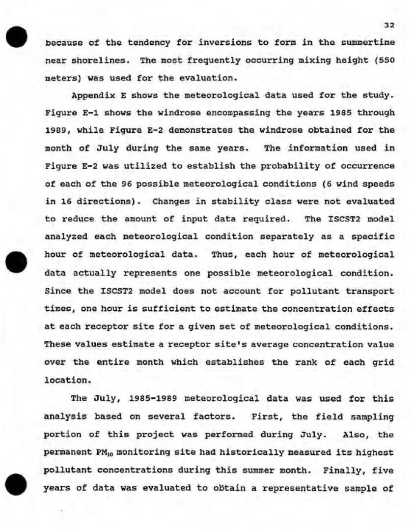
because of the tendency for inversions to form in the summertime near shorelines. The most frequently occurring mixing height (550
meters) was used for the evaluation.
Appendix E shows the meteorological data used for the study. Figure E-1 shows the windrose encompassing the years 1985 through 1989, while Figure E-2 demonstrates the windrose obtained for the
month of July during the same years. The information used in
Figure E-2 was utilized to establish the probability of occurrence
of each of the 96 possible meteorological conditions (6 wind speeds in 16 directions). Changes in stability class were not evaluated to reduce the amount of input data required. The ISCST2 model
analyzed each meteorological condition separately as a specific
hour of meteorological data. Thus, each hour of meteorological
data actually represents one possible meteorological condition.
Since the ISCST2 model does not account for pollutant transport
times, one hour is sufficient to estimate the concentration effects
at each receptor site for a given set of meteorological conditions.
These values estimate a receptor site's average concentration value
over the entire month which establishes the rank of each grid
location.
The July, 1985-1989 meteorological data was used for this
analysis based on several factors. First, the field sampling
portion of this project was performed during July. Also, the
permanent PMjo monitoring site had historically measured its highest
pollutant concentrations during this summer month. Finally, five
meteorological conditions experienced in the region. This reduces
the likelihood of non-representative input data due to possible non-normal events in a particular year. Figures E-3 through E-6 give the corresponding windroses for the years of 1985 and 1989, respectively. These figures show that the annual windroses are
similar, but change when analyzing only the month of July.
Therefore, a minimum of five years of meteorological data should be
used whenever possible.
4.2.3 Topography
The topography of the region is fairly level, except for
lowlands along the Hudson River to the east (in the Lincoln Harbor
and Port Arthur areas) and the beginning of the meadowlands to the west. According to figure 3-1, these regions have little to no
human population. In the main portion of the study area, the
overall elevation change is approximately 50 feet. Figure 4-1 shows the elevation changes within the region. Because of the level terrain in the populated portions of the study area, topography was not factored into the dispersion model.
4.2.4 Special Model Requirements
An output file was generated in order to use the SITE model to
establish the monitor locations. As shown in Appendix B and
34
4.3 Location Evaluation
4.3.1 Receptor Rankings
As previously described, the estimated concentrations experienced at each receptor location are based on the anticipated
concentration from the dispersion model for a given set of meteorological conditions and the probability of occurrence of that
set of meteorological conditions. The potential monitor sites (represented by the receptor grids) are ranked based on the results
of these calculations.
4.3.2 Location Determination
The SITE computer program identified the final monitor
locations. Information on the use of this model, as well as the FORTRAN source code, is found in Appendix C.
The final results of the site selection process are shown on
the map of Figure 4-3. The procedure was performed for
concentrations determined using point source emission rates based
ͣ
M«>Vl If }9
jU t«>»>M M«> «0S CMAs It?. 14%.
ͣ
fii^w «N« ^&m 10* nr«>^«*t tfttfw Umg iM»A« iww
IBOfr«vtv Vmwhi ticmwvw t^n9\m r*« MM. im It.
*"•• l»i» tM •"»• Mtfcn »»n
-O *«TW» •»• -O W * ••'^ C **<*• ͣ*« WEEHAWKEN. N J-N. Y
Dtn Pt
^
M A N H
?5,ar
\"»10»<W
SCALE 1.24000
0
2000 MOO
I
fOOO
CONTOUR IMTERVAL 10 FEET
NtTIOMM. GEOOniC VEKTICAl. MTUM Of 1929
KfTH CURVES AND SOUNDINGS IN rctr—MTUM IS MEAN LOW WATER
THl MLATlOMSHir tttwCCN TM[ TWO BATUMS IS »«>l»llC
(MOMLIMC SHOVN KCMCSCNTS THC AmOXiMtTC IINC Or HttN MICN «tT(* TM MCUl MNCC Of TIDE It ArPDOIlHtTCLr 4.2 fCCT IN TMC MUOSON aiVC*
AND S.I rtn IM THE MACKCNSAC* A>IO M$t*IC (IVtXS
THIS MAr eOMn.lES WITH MATIONAt. MAP ACCUHACT STANDARDS K>R SAL£ av U. S. GEOLOGICAL SURVEY
KMVtR. COLOAAOO Km. OR RESTON. VIRGINIA 23M2
• rOkTftM KKMWMC TOK>GIU^HK MATS ANO SYMBOLS S AVAAABlf OM REQUEST
FIGURE 4-3 - Final monitor locations for the Weehawken, NJ field study. Site
36
5.0 Field Study Results
5.1 Introduction
A PMio evaluation study conducted in the Weehawken, New Jersey
area from July 1-24, 1992 determined the particulate loadings in
the vicinity of the Lincoln Tunnel entrance. The U.S.
Environmental Protection Agency's Aerosol Physics and Methods Branch of the Atmospheric Research and Exposure Assessment Laboratory (AREAL), as well as the Monitoring and Reports Branch of the Office of Air Quality Planning and Standards (OAQPS) sponsored the study. EPA Region II and the New Jersey Department of Environmental Protection also participated.
The Weehawken, NJ area is an urban region located west of New York City, NY across the Hudson River from the island of Manhattan. As shown in Figure 4-1, Interstate 495 intersects the region, carrying traffic to and from NYC through the Lincoln Tunnel. Often the traffic on this roadway backs up around the entrance loop, especially from 6 to 9 a.m. and 3 to 7 p.m., as people commute to work.
The air monitors used for the study were the LRAPA Portable
Samplers, Model 3.1, described in LRAPA (1992). These battery
operated samplers are designed to achieve a 10 jum particle size cut
point at a flow rate of 5 liters per minute (1pm) . A rotameter
determines the flow rates. A pressure orifice located at the
exhaust end of the sampler maintains constant flow by measuring
pressure drop. Since the pressure drop across the orifice is a
ensures a constant sampling flow rate through the system. The circuitry of the sampler adjusts the flowrate to guarantee a constant orifice pressure drop. If the monitor cannot maintain a suitable flowrate, it automatically shuts down- Reasons for a low flow rate may be excessive filter loadings, damage to the monitor, or an insufficient voltage output from the battery. The monitors are equipped with low voltage battery indicator lights to identify failures due to insufficient battery output. The samplers are also equipped with a programmable timer and an elapsed time accumulator to record exposure periods. The Operations Manual for the samplers (LRAPA, 1992) should be consulted for further information on the physical characteristics, as well as the operating procedure, for the monitors.
5.2 Study Objectives
The main objective of the field study was to characterize the PMjo pollutant concentration levels in the study area by utilizing the portable LRAPA air quality samplers. The results of the field study tested the guidance methodology presented in this document
for establishing a PMjg monitor network which provides adequate
information for determining the concentration gradients within a
neighborhood scale study area. The data obtained from the study
determined a) if the PM,o reference monitor within the study region
needs to be relocated to another site or Jb) if the concentration
measurements warrant the existence of a reference monitor within
38
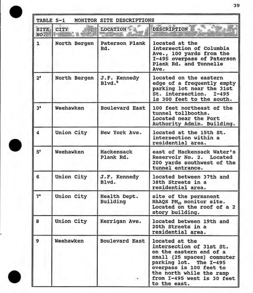
5.3 Final Site Selection
The protocol indicated for the SITE model determined the monitor locations used for the field study. Figure 4-3 shows the twelve monitor sites chosen for the study, including the permanent
PMjo monitor located on Central Ave. in Union City (site number 7) . Table 5-1 describes the final locations used in the study.
5.4 Concentration Results
Appendix A shows the PMio concentration isopleths experienced
within the study region. Figures A-1 through A-2 0 show the
isopleths for each individual sampling day. Figure A-21 gives the average concentration isopleth for the region during the entire 20 day study. The values shown in Figure A-21 represent the average normalized values over the study period. These normalized values are obtained by dividing the concentration reading at a particular location by the average concentration measurement for all monitor sites for a particular day. These normalized values are averaged for each site based on the number of successful sampling days at that site. This procedure avoids any bias resulting from days when no valid samples were collected. If a monitor did not run on days with high pollutant levels, that site may show a low overall average concentration even if it consistently measured higher than average values on the lower reading days. Therefore, the
normalized concentration values provide relative readings at each site which reduces bias based on the pollutant's temporal
TABLE 5-1 MONITOR
SITE DESCRIPTIONS |
SITE CITY LOCATION DESCRIPTION
NO.
1 North Bergen Paterson Plank located at the 1
Rd. intersection of Columbia
Ave., 100 yards from the 1-495 overpass of Paterson
Plank Rd. and Tonnelle
Ave.
2* North Bergen J.F. Kennedy located on the eastern
i
1
Blvd.** edge of a frequently empty parking lot near the 31st
St. intersection. 1-495
is 300 feet to the south. |
1 3*
Weehawken Boulevard East tunnel tollbooths.100 feet northeast of theLocated near the Port
Authority Admin. Building. [
4 Union City New York Ave. located at the 15th St.
intersection within a
residential area. [
5^ Weehawken Hackensack east of Hackensack Water•s
Plank Rd. Reservoir No. 2. Located
200 yards southwest of the tunnel entrance.
6 Union City J.F. Kennedy located between 37th and
Blvd. 38th Streets in a
residential area. ||
T Union City Health Dept. site of the permanent
Building NAAQS PMjo monitor site.
Located on the roof of a 2
story building. ||
8 Union City Kerrigan Ave. located between 19th and
20th Streets in a i
residential area. |
9 Weehawken Boulevard East located at the
intersection of 31st St.
on the eastern end of a
small (25 spaces) commuter
parking lot. The 1-495
overpass is 100 feet to
the north while the ramp
"* from 1-495 west is 30 feet
40
TABLE 5-1 MONITOR SITE DESCRIPTIONS (cont) \
10^ Union City Central Ave. located at the 14th St.
intersection next to a 3
story church building. 11 Union City Palisade Ave. located at the 27th St.
intersection in a residential area.
12 Union City West Ave. located at the 25th St.
intersection next to a
small restaurant. A nightclub is located on the opposite corner.
* Monitors are collocated at these sites
'' The original location for site 2 was inaccessible because
the roadway in the area had been blocked off and rerouted. Therefore, the final site selected was based
on the location within a grid which had the highest
correlation coefficient with the original location and was accessible by car.
'ͣ Sites did not conform to the general siting criteria
established in the CFR.
5.5 Data Quality
5.5.1 Sample Collection
Total valid data capture for the study was slightly below 90%
(31 samples deemed invalid out of 300 samples taken). Table 5-2
lists the reasons samples were invalidated, as well as the number of samples affected in each category. Over 50% of the invalidated samples resulted from the inaccessibility of the monitors at site 7 during the weekends and holidays. When these samples are not considered in the data capture analysis, almost 95% of the samples are valid. Monitor failure only accounted for 16% of the invalid
TABLE 5-2 |
ERROR DESCRIPTION NUMBER OF
SAMPLES
INVALIDATED
PERCENT INVALIDATED
Site 7 not accessible 16 51.6
Monitor not set correctly (operator
error)
8 25.8
Monitor Failure (low battery
indication)
5 16.1
Filter Damaged (operator error) 2 6.5
TOTAL 31 100.0
5.5.2 Analytical Precision
Three types of control filters established the analytical precision of the study: unexposed lab blanks, unexposed field
blanks and exposed field blanks. Unexposed lab blanks were filters
which remained in a controlled environment except for being weighed
at the beginning and end of a sampling day. These filters provide
information on the precision of the weighing technique. Unexposed
field blanks were loaded in the monitor inlets, placed in plastic
bags and carried into the field, but were never attached to the
samplers. These filters indicate any damage which occurred to the
filters as they were loaded and unloaded into the inlets. Exposed
field blanks underwent the same treatment as the unexposed field
blanks but were also attached to the monitors and placed in the field although the monitors were not run. These filters represent the amount of contamination which occurred while the monitors did
42
replaced). Thus, analytical precision is estimated from
reweighings of the three types of blank filters, and is given in
Table 5-3.
The maximum weighing difference experienced during the study
was 0.029 mg which occurred on an exposed filter. This difference corresponds to a concentration of less than 5 fig/m^ under typical
operating conditions (20 hour sampling at 5 1pm). The average
difference on exposed filters of 0.013 mg corresponds to a concentration of only 2.17 iiq/v:?. Neither the lab or field blanks showed a substantial inconsistency in measurements. Thus, the
overall analytical precision for the project is good. A surprising
result was the lack of negative differences in the blanks. One reason may be that the filters were not weighed in a controlled
environment, only stored in one. However, all differences were
small and deemed insignificant. For more information on the
analytical procedures used for the experiment. Appendix F should be
consulted.
TABLE 5-3
FILTER BLANKS EXPOSED
FILTERS
LAB FIELD
1 Number of
Samples
40 40 «
Average Diff. 0.005 0.007 0.013
Std. Deviation 0.004 0.005 0.008
Maximum Diff. 0.015 0.018 0.029
1 Minimum Diff.
0.000 0.000 0.0055.5.3 Monitor Performance
5.5.3.1 Study Design
As previously mentioned, monitors were located at 12 separate
sites throughout a 2 km X 2 km study area. The site identification
number represented the expected concentration level at that site (based on dispersion modeling) compared with the other sites.
Thus, the highest expected pollutant concentration should occur at
site 1 and the lowest concentration at site 12. For each of the twenty sampling days, the monitors ran for 20 hours, from 10 a.m. until 2 p.m. of the following day. After the removal of a sample
from a monitor, the location of that monitor changed to the next site. Thus, after collecting the sample at one site, the monitor
from this site moved to the next site. The monitor at this new
site then transferred to another site, and so on. Therefore, each
monitor had a theoretically equal chance to be sited at each sampling location during the study.
To ensure the monitors performed adequately in the field, flow rates were checked before and after sampling with a bubble flowmeter (Mini-Buck Calibrator, 0-3 0 1pm). As seen in Appendix B, the maximum flow measured was 5.18 1pm while the minimum flow was recorded at 4.67 1pm. Thus, all samplers consistently had flow
rates well within + 10% of 5 1pm as recommended in the Operations
Manual (LRAPA, 1992).
To determine any sampling bias by the LRAPA monitors during
44
establish the performance characteristics and reliability of the
monitors prior to the field study. Two tests were run with all
available monitors collocated such that all inlets were a minimum
of 1 meter apart, thus ensuring all monitors sampled the same
ambient aerosol concentration. Table 5-4 shows the results of
these tests. Second, the concentration values obtained from the field study at each site for the collocated monitors is compared. Figures 5-1, 5-2 and 5-3 show the results for site 2, 3 and 7, respectively. For the figures, locations a and b at the collocated
sites were determined before the study began.
Finally, a study performed in Research Triangle Park, N.C. followed the Weehawken, NJ field study to determine the LRAPA
samplers performance compared to reference high volume samplers.
For this study, two LRAPA monitors were collocated with two
reference samplers. One reference sampler had a Wedding PMjo size
selective inlet while the other had an Andersen-Sierra PMjq size
selective inlet. Two meters separated the reference samplers while
the LRAPA monitors were located approximately 1.5 meters from each of the reference samplers. All monitors sampled for 23 hours each
day. The LRAPA monitors ran at the recommended 5 1pm while the
high volume samplers ran at 40 cfm. Average daily wind speeds
5.5.3.2 Study Results
Table 5-4 presents the results of the preliminary performance
study done at the Research Triangle Park, NC facilities. The
monitors provided comparable readings for this study, with only
monitors 70, 91 and 409 showing a very slight high sampling bias. For the field study in Weehawken, NJ, the monitors performed consistently throughout the study. As shown in Table 5-2, only 16% of the invalidated samples were the result of monitor failure.
Also, Figures 5-1 through 5-3 demonstrate that most of the
collocated monitors provided similar concentration readings. No monitor regularly sampled higher or lower PM,o concentrations
throughout the study. Of the 50 successful collocated samples
taken during the study, over 10% of the monitors produced equivalent concentration values while 90% showed no more than a 5
/xg/m' difference between samples. Based on these results, the
samplers seemed to perform well under both high and low pollutant loading conditions.
The results of the field study also seem to indicate that
LRAPA monitor readings were comparable to the actual particulate concentrations in the area based on the results from the NAAQS permanent monitor located at site 7. Table 5-5 shows the concentration values read by the NAAQS monitor. This monitor ran
for 24 hours every sixth day from midnight to midnight. Therefore,
the concentration values are not directly comparable. Also, some
of the sampling days for this monitor occurred on weekends when
46
1 TABLE 5-4 -
MONITOR EVALUATION (at EPA Facilities)
MONITOR
1 NUMBER
TEST 1
Ambient Concentration
TEST 2
Ambient Concentration
{/xg/m')
1 ^^
30 2460 34 32
63 28 37
68 27 38
70 31
34 1
71 ** 24
73 28 35
86 **
29
91 29 35
93 28 33
1 408
23 37409 29
33
410 28 35
AVERAGE 28.68 32.82
STD. DEV. 2.72 4.49
** Monitors
Monitors
71 and 86 were not run during this test.
64, 67 and 72 were unavailable for this study.
Because concentration readings could not be directly compared
to the reference monitor at site 7, the separate study measuring
the two types of monitors was performed in North Carolina. As can
be seen in Figure 5-4, the LRAPA monitors showed the same general
trend in concentration readings but consistently underestimated the
actual values. Since wind speeds were low during the study, local
weather effects were probably not an influence on the study
FIGURE 5-1
MONITOR COMPARISON
Collocated Data - Site 2
E
80-
?70-O-H----r
123456789 10 1112 13 14 15 16 17 18 19 20 DAY
Location a —•- Location b
FIGURE 5-2
MONITOR COMPARISON
Collocated Data - Site 3
T---1---r-23456789 10 1112 13 14 15 16 17 18 19 20
DAY
48 FIGURE 5-3
^-90
E 80
§"70
60 50 40 30
o
<->20
o
I 0
MONITOR COMPARISON
Collocated Data - Site 7
5 6 7 8 11 12 13 14 18
DAY
Location a -•— Location b I
TABLE 5-5 - CONCENTRATION READINGS FROM THE NAAQS PERMANENT
MONITORING SITE IN UNION CITY, NJ *
DATE
CONCENTRATION VALUE (in /ig/m')
July 5 41
1 July 11
25July 17 27
1 July 23
18FIGURE 5-4 - Comparison of PM,o concentration readings from
high volime szunplers to the LRAPA Seunplers (from study
performed in Research Triangle Park, NC).
Reference vs. LRAPA Sampler Comparison
30.0
28.0-
p26.0-ͣ
\24.0H
322.0-Q 20.0
I-a 18.0
S
16.0-o
o
14.0-o
12.0H
10.0
3
DAY
Wedding "••" Andersen LRAPA #408 LRAPA #409