DEPENDENCE OF FUNGAL PLANT PATHOGEN HOST BREADTH ON PLANT CHARACTERISTICS
Nguyen Huynh An Markus Le
A thesis submitted to the faculty at the University of North Carolina at Chapel Hill in partial fulfillment of the requirements for graduating with Honors in the Department of Biology in the
College of Arts and Sciences
Chapel Hill 2014
Approved by:
ABSTRACT
Over time, travel between continents has become easier, allowing many diseases and pests to leave their native habitats, sometimes with disastrous results. Famous examples include the chestnut blight and woolly adelgids, which have greatly harmed ecosystems in the United States. I investigated the factors that allow these invasive species to flourish in non-native environments by examining how a plant’s susceptibility to pathogens depends on its phylogeny, traits, and native geographic range. To do so, I used grasses that varied widely across these three factors in an observational field study and in vitro inoculation experiment. Collected
susceptibility data was compared to traits like leaf mass per area (LMA), growth rate, and photosynthetic rate. Initial results indicate significant susceptibility differences among different grass species. The results will help illuminate what allows pathogens to infect new hosts, allowing planning for the prevention and mitigation of species invasion.
INTRODUCTION
As time goes on, the barriers separating continents have become less and less significant. Journeys that used to take weeks to complete by ship can now be completed in mere hours on an airplane, at relatively low cost. However, people are sometimes not the only passengers that cross continents. Whether intentionally or by accident, many species have been allowed to leave their native habitat, sometimes with disastrous results. This process is known as species invasion, which occurs when species from a foreign environment establish a foothold in a new geographic area where they were not originally present. While sometimes species invasions can be
causing great harm to ecosystems in the United States, as well as bay barnacles which cause great economic costs due to their effect on man-made structures along the water.
Not every species that moves to a foreign geographic location successfully takes hold there, however. Most species fail to thrive in a foreign environment and die out. For those that do successfully survive, there are five hypotheses on why they do so. The first is the Innate Biology Hypothesis, which describes the traits inherent to the organism as the crucial determining factor. For example, an invader may be very “weedy” and generalist, allowing it to thrive in a wide variety of environments, or it may be pre-adapted to the environment to which it is being introduced (Kolar and Lodge 2001). The second hypothesis is called the Enemy Release and Biotic Resistance Hypothesis, which attributes the success of a species to take hold to the lack of predators and competition, and the resistance of invading species to diseases already in the community, or lack thereof (Montserrat, Maron, and Marco 2005). The Community Invasibility hypothesis relates empty or underutilized niches in a community, or other traits that make a community prone to invasion to the success of a species invasion (Davis, Grime, and Thompson 2000). The Propagule Pressure hypothesis correlates increased exposure frequency and intensity to an environment to how likely it will be to establish itself in the community (Verling et al. 2005). Finally, the Rapid Evolution hypothesis states that often species that successfully invade an environment can and do evolve rapidly to adapt to the local environment, allowing them to survive over generations (Davidson, Jennions, and Nicotra 2011).
My research project aims to examine the factors that allow these invasive species to flourish in non-native environments and conditions, more specifically the Community
infecting plants by attempting to answer the question “What aspects of a plant will allow it to be infected by any given pathogen?” Several hypotheses have been posed to answer this question. For example, the phylogenetic relationship between different tropical plant species was a strong determinant of infection rates by specific pathogens in one study, meaning that closely related plants experienced similar infection rates (Gilbert and Webb 2007). Similarly, Kumar et al (2011) hypothesized that individual plant traits could be correlated to the susceptibility of a plant to pathogens, however they found no significant relationship, since it is possible that
susceptibility is determined by a combination of factors rather than individual traits. My aim is to incorporate and expand on these studies by testing my hypothesis that pathogen susceptibility depends on not just phylogeny or plant traits, but rather both simultaneously, as well as a third component, the native geographic range of the plants, which could point towards the importance of coevolution between plants and pathogens. The plant pathogen that I have chosen for the project is Fusarium graminearum. Fusarium graminearum is a generalist pathogen that infects mostly wheat, oat, and barley in cooler regions of the world and is responsible for the destructive plant disease called Fusarium head blight (Cuomo et al. 2007).
MATERIALS AND METHODS
Plants and Plant Traits
The plants were chosen to allow for comparison across the three variables: relatedness, plant traits and native geographic range. For example, I would compare closely related species with similar traits, but different native geographic ranges to observe the effect of the plants’ geographic ranges. Plants with similar traits and native geographic ranges, but that are not closely related could be chosen to observe the effect of phylogeny. To observe the effect of the plants’ traits, I would compare plants that are closely related and have similar native geographic ranges, but differ in traits. As I am interested in the effects of the traits themselves on
susceptibility rather than differences between species, the plants used were not genetically identical, to allow for trait variation and a more continuous trait distribution among plants.
Native geographic range estimates, the tribe to which each grass species belonged, as well as the photosynthetic pathway (C3 or C4) for each grass host species were obtained from floristic guides and other literature. For the field plant traits, growth rate, leaf mass per area and photosynthetic rate were measured, while pre-existing data were obtained from a fellow lab member, Miranda Welsh. Leaf mass per area was obtained by scanning leaf segments of each plant into a computer, calculating the area of the leaf segments with computer software and using a balance to obtain the mass of that same leaf segment. Photosynthetic rate was measured using an infrared gas analyzer (IRGA), which measures the change in gas composition in a closed chamber containing a leaf being exposed to light.
Detached Leaf Assay
dishes were prepared with water agar that contained kinetin as a senescence retarder for the leaf segments, and the fungal spores were diluted in water, since the fungi spread their spores through water in nature. The spores were diluted to a specific concentration (50000 spores per mL), with Tween 20 as an emulsifier to prevent the spore suspension from rolling off the leaves in the petri dish. The fungal spores came from separate isolates that were grown separately in petri dishes, but the spores were mixed together in the spore suspension to allow the fungus to be as generalist as possible. The fungus was a novel pathogen to all of the plants, which models how a foreign pathogen is affected by plant traits in general.
Each petri dish contained two leaf segments, each of which was inoculated using one drop of the fungal spore suspension. The petri dishes incubated for about two weeks to allow for the development of symptoms. These procedures were modeled after those used by Kumar et al (2011). Every day during the incubation period, the presence of fungal lesions was recorded, along with the approximate length and width of the lesions. For the data analysis, a day was chosen during the two week period on which all leaves that were going to become infected had already become infected, but the size of the lesions that had developed had not yet become limited by the size of the leaf segment. This allowed the length and width measurement to remain a measure of susceptibility rather than the size of the leaf itself.
Field Experiment
were transferred into the field. The area in the field chosen for the experiment had uniform vegetation, which was kept as intact as possible while putting the pots into the ground, to simulate a non-disturbed environment as best as possible. This allowed wild diseases from the environment to infect the experimental plants. Since plants in the field were both native and exotic, and the diseases in the field are mostly native, this would show the difference between infection by native and novel pathogens.
The pots were left in the field for six weeks, and every two weeks the plants were
visually assessed for fungal leaf damage. Damage was recorded for every individual leaf on each plant as a percentage of the leaf area damaged by fungi. The field plants were also used to measure growth rate. A single leaf on each plant was tracked throughout the six weeks, and while taking damage data, the length and width of the leaves was measured.
Measuring susceptibility
the field experiment, this was achieved by choosing a spot of uniform vegetation in the field, and by leaving vegetation around the pots intact, which helped standardize the types and amounts of pathogens, as well as transmission rates between plants. The plants were also randomized in the field plots, to further prevent location from skewing data for any one species.
Unless otherwise stated, I performed all work described in this thesis.
RESULTS
Detached Leaf Assay
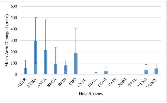
Before looking at the interactions between origin, phylogenetics, and plant traits, I looked at the effect of each of these individually. There is high variation in damage between individual species; however, the differences are not statistically significant (Fig. 1). However, the same is not true when looking at the grass tribes. When the individual species are grouped together into their appropriate tribes, there is a statistically significant difference (p<0.05) in damaged leaf area between the tribes (Fig. 2). Looking at the comparisons between the data sorted by
categories, origin and photosynthetic pathway, showed that there was no meaningful difference between the categories, as with the comparison between species (Fig. 3, Fig. 4). Figures 5 through 7 show scatter plots comparing the damage data to the numerical trait data,
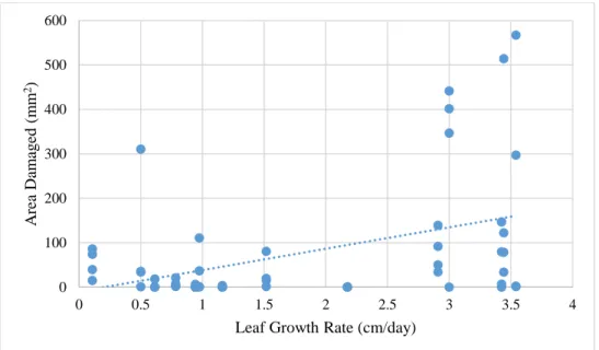
photosynthesis rate, LMA, and leaf growth rate. Of these three, only the relationship between leaf growth rate and damage was significant (r2=.1776, p<0.05). Generally, as leaf growth rate increased, the amount of damage on the leaves increased.
differences in susceptibility through multiple linear models, which are statistical tests that allow for the comparison of the effects of several independent variables on the dependent variable, or in this case, damage of plant leaves caused by fungi.Of the nine models, only the models for leaf growth rate by origin, and LMA, photosynthesis rate, and leaf growth rate by photosynthetic pathway (Figs. 13, 14, 15, and 16 respectively) were statistically significant (p<0.05), showing interactions between leaf growth rate and origin, (r2=0.2893), LMA and photosynthetic pathway (r2=0.1627), photosynthesis rate and photosynthetic pathway (r2=0.1924), and leaf growth rate
and photosynthetic pathway (r2=0.2936) in determining the amount of damage. However, due to the low number of samples available for C4 plants (only three of the species used were C4), the significance of the interactions and the models involving photosynthetic pathway may be exaggerated.
Also noteworthy is the model for LMA by continent of origin (Fig. 12). The model is not statistically significant, but it is marginal (r2=0.1537, p=0.06972), and the interaction term between LMA and origin is significant (p<0.05) which may potentially point to interaction between the two traits influencing damage. For plants from the Americas, damage decreases as LMA increases, while for plants from Europe and Asia, damage increases as LMA increases. Field Experiment
two variables was also statistically significant (p<0.05). The model follows the same pattern as it did for the detached leaf assay: For American plants, damage decreases as LMA increases, damage increases as LMA increases for Eurasian plants.
DISCUSSION
In agreement with the experiment conducted Gilbert and Webb (2007), relatedness between species can help predict how susceptible they are to disease, as can be seen from the damage comparison between tribes in the detached leaf assay. The results also agree with those found by and Kumar et al (2011) that single plant traits are generally unable to predict
susceptibility to disease, especially in the field. Integrating the results from these experiments in more complex models yields some interesting results.
there to be a negative correlation plants for American plants, and a positive correlation for European plants, because American plants have been able to adapt and develop resistance to local pathogens, which would make a higher LMA an asset, while for Eurasian plants which are more susceptible to local diseases, a higher LMA would be a burden.
While the most of the other models are statistically insignificant, it is interesting to note that most of the models follow the same trend as the LMA by origin models: comparing the regressions for same models between the two experiments shows that most of them share the same pattern. Where there is negative correlation in the detached leaf assay, there is negative correlation in the field experiment, and where there is positive correlation in the detached leaf assay, there is positive correlation in the field experiment. Due to the statistical insignificance of these models, it is uncertain whether these patterns are due to coincidence, but the possibility exists that patterns may be present and that they just require further research, which makes for several interesting projects that could be done in the future.
Another interesting questions that arises from these results. As mentioned before, the experiments were designed with the same ideas and principles in mind. However, the controlled petri dishes and the field are two very different environments. In the detached leaf assay, there was only one known generalist pathogen that infected the plants, while field is filled with a very wide variety of fungal diseases, many of which are highly specialized to specific grass species. This alone would lead one to expect the results between the lab and the field to be very different. If further experiments were to prove all of the similarities between the two statistically
APPENDIX
The table below (Table 1) shows a list of all abbreviations used in the figures and the full name of species that they represent.
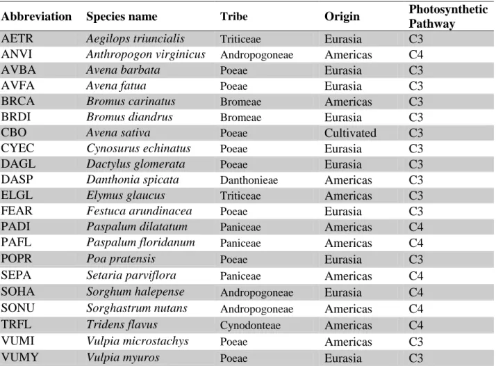
Table 1. Plant species abbreviations for species names used in figures below, along with basic relevant information to the experiments.
Abbreviation Species name Tribe Origin Photosynthetic
Pathway
AETR Aegilops triuncialis Triticeae Eurasia C3
ANVI Anthropogon virginicus Andropogoneae Americas C4
AVBA Avena barbata Poeae Eurasia C3
AVFA Avena fatua Poeae Eurasia C3
BRCA Bromus carinatus Bromeae Americas C3
BRDI Bromus diandrus Bromeae Eurasia C3
CBO Avena sativa Poeae Cultivated C3
CYEC Cynosurus echinatus Poeae Eurasia C3
DAGL Dactylus glomerata Poeae Eurasia C3
DASP Danthonia spicata Danthonieae Americas C3
ELGL Elymus glaucus Triticeae Americas C3
FEAR Festuca arundinacea Poeae Eurasia C3
PADI Paspalum dilatatum Paniceae Americas C4
PAFL Paspalum floridanum Paniceae Americas C4
POPR Poa pratensis Poeae Eurasia C3
SEPA Setaria parviflora Paniceae Americas C4
SOHA Sorghum halepense Andropogoneae Eurasia C4
SONU Sorghastrum nutans Andropogoneae Americas C4
TRFL Tridens flavus Cynodonteae Americas C4
VUMI Vulpia microstachys Poeae Americas C3
Detached Leaf Assay
Figure 1. Comparison of damage between species, with standard error bars. The differences in damage between the plant species are not statistically significant.
Figure 2. Comparison of damage between tribes, with standard error bars. The differences in damage between the plant species are statistically significant (p<0.05).
0 100 200 300 400 500 600
Me
an
A
rea
Dam
ag
ed
(
m
m
2)
Host Species
0 100 200 300 400 500 600
A
v
er
ag
e
A
rea
Dam
ag
ed
(
m
m
2)
Figure 3. Comparison of damage between plants of different origins, with standard error bars. The differences in damage between the plant species of different origins is not statistically significant.
Figure 4. Comparison of damage between species with different photosynthetic pathways, with standard error bars. The differences in damage between the photosynthetic pathways is not statistically significant.
0 50 100 150 200 250 300 350 400 450
Americas Eurasia Cultivated
A
v
er
ag
e
A
rea
Dam
ag
ed
(
m
m
2)
Origin
0 50 100 150 200 250 300
C3 C4
A
v
er
ag
e
A
rea
Dam
ag
ed
(
m
m
2)
Figure 5. Comparison between damage and photosynthesis rate, with linear regression. Photosynthesis rate does not significantly contribute to the variation in damage. The equation for linear regression for this model is y = -2.6976x + 95.477, with R² = 0.0004.
Figure 6.Comparison between damage and photosynthesis rate, with linear regression. LMA does not significantly contribute to the variation in damage. The equation for linear regression for this model is y = -31.157x + 152.61, with R² = 0.0095.
0 100 200 300 400 500 600
4 5 6 7 8 9 10
A
rea
Dam
ag
ed
(
m
m
2)
Photosynthesis Rate (PN)
0 100 200 300 400 500 600
1.5 2 2.5 3 3.5 4
A
rea
Dam
ag
ed
(
m
m
2)
Figure 7. Comparison between damage and leaf growth rate, with linear regression. Leaf growth rate significantly contributes to the variation in damage (p<0.05). The equation for linear regression for this model is y = 47.969x - 9.5014, with R² = 0.1776.
Detached Leaf Assay by Tribe
Figure 8. Comparison between damage and photosynthesis rate, separated by tribe, with linear regressions. The equation for the Triticeae linear regression for this model is y = 31.546x - 174.85, with R² = 0.2579. The equation for the Poeae linear regression for this model is y = -24.433x + 252.64, with R² = 0.0397. The equation for the Bromeae linear regression for this model is y = -55.003x + 418.35, with R² = 0.0079. Due to insufficient data points, no linear regressions were made for Andropogoneae, Paniceae and Cynodonteae.
0 100 200 300 400 500 600
0 0.5 1 1.5 2 2.5 3 3.5 4
A
rea
Dam
ag
ed
(
m
m
2)
Leaf Growth Rate (cm/day)
0 100 200 300 400 500 600
4 5 6 7 8 9 10
A
rea
Dam
ag
ed
(
m
m
2)
Photosynthesis Rate (PN)
Triticeae
Andropogoneae
Poeae
Bromeae
Paniceae
Cynodonteae
Linear (Triticeae)
Linear (Poeae)
Figure 9. Comparison between damage and LMA, separated by tribe, with linear regressions. The equation for the Triticeae linear regression for this model is y = -470.67x + 1283.1, with 0.2579. The equation for the Poeae linear regression for this model is y = 116.69x - 187.07, with R² = 0.0775. The equation for the Bromeae linear regression for this model is y = -96.537x + 307.96, with R² = 0.0079. Due to insufficient data points, no linear regressions were made for Andropogoneae, Paniceae and Cynodonteae.
Figure 10. Comparison between damage and leaf growth rate, separated by tribe, with linear regressions. The equation for the Triticeae linear regression for this model is y = 19.041x - 6.9255, with 0.2579. The equation for the Poeae linear regression for this model is y = 53.45x - 21.753, with R² = 0.2037. The equation for the Bromeae linear regression for this model is y = -6.8647x + 98.815, with R² = 0.0079. Due to insufficient data points, no linear regressions were made for Andropogoneae, Paniceae and Cynodonteae.
0 100 200 300 400 500 600
1 1.5 2 2.5 3 3.5 4
A rea Dam ag ed ( m m 2)
Leaf Mass per Area (g/m2)
Triticeae Andropogoneae Poeae Bromeae Paniceae Cynodonteae Linear (Triticeae) Linear (Poeae) Linear (Bromeae) 0 100 200 300 400 500 600
0 1 2 3 4
A rea Dam ag ed ( m m 2)
Leaf Growth Rate (cm/day)
Detached Leaf Assay by Origin
Figure 11. Comparison between damage and photosynthesis rate, separated by origin, with linear regressions. The equation for the Americas linear regression for this model is y = 50.114x - 272.97, with R² = 0.0836. The equation for the Eurasia linear regression for this model is y = -22.887x + 225.77, with R² = 0.0582. Due to insufficient data points, no linear regression was made for cultivated species.
Figure 12. Comparison between damage and leaf mass per area, separated by origin, with linear regressions. The equation for the Americas linear regression for this model is y = -161.52x + 501.85, with R² = 0.2873. The equation for the Eurasia linear regression for this model is y = 121.26x - 207.13, with R² = 0.0941. Due to insufficient data points, no linear regression was made for cultivated species. This model is marginally statistically significant (Multiple R² = 0.2873, p = 0.0697).
0 100 200 300 400 500 600
4 5 6 7 8 9 10
A
rea
Dam
ag
ed
(
m
m
2)
Photosynthesis Rate (PN)
Americas
Eurasia
Cultivated
Linear (Americas)
Linear (Eurasia)
0 100 200 300 400 500 600
1 1.5 2 2.5 3 3.5 4
A
rea
Dam
ag
ed
(
m
m
2)
Leaf Mass per Area (g/m2)
Americas
Eurasia
Cultivated
Linear (Americas)
Figure 13. Comparison between damage and leaf growth rate, separated by origin, with linear regressions. The equation for the Americas linear regression for this model is y = 108.63x - 53.301, with R² = 0.4423. The equation for the Eurasia linear regression for this model is y = 32.863x - 5.8817, with R² = 0.1149. Due to insufficient data points, no linear regression was made for cultivated species. This model is statistically significant (Multiple R2 =
0.2893, p = 0.001382).
Detached Leaf Assay by Photosynthetic Pathway
Figure 14. Comparison between damage and photosynthesis rate, separated by photosynthetic pathway, with linear regressions. The equation for the C3 linear regression for this model is y = -14.044x + 166.84, with R² = 0.0157. The equation for the C4 linear regression for this model is y = 492.03x - 3598.1, with R² = 0.5853. This model is
statistically significant (Multiple R2 = 0.1924, p = 0.01063).
0 100 200 300 400 500 600
0 1 2 3 4
A
rea
Dam
ag
ed
(
m
m
2)
Leaf Growth Rate (cm/day)
Americas
Eurasia
Cultivated
Linear (Americas)
Linear (Eurasia)
0 100 200 300 400 500 600
4 5 6 7 8 9 10
A
rea
Dam
ag
ed
(
m
m
2)
Photosynthesis Rate (PN)
C3
C4
Linear (C3)
Figure 15. Comparison between damage and LMA, separated by photosynthetic pathway, with linear regressions. The equation for the C3 linear regression for this model is y = 86.816x - 133.86, with R² = 0.0475. The equation for the C4 linear regression for this model y = -210.25x + 690.78, with R² = 0.4889. This model is statistically
significant (Multiple R2 = 0.1627, p = 0.02529).
Figure 16. Comparison between damage and leaf growth rate, separated by photosynthetic pathway, with linear regressions. The equation for the C3 linear regression for this model is 33.821x + 7.2679, with R² = 0.1136. The equation for the C4 linear regression for this model y = 132.43x - 109.61, with R² = 0.6189. This mode is statistically significant (Multiple R2 = 0.2936, p = 0.0003936).
0 100 200 300 400 500 600
1 1.5 2 2.5 3 3.5 4
A
rea
Dam
ag
ed
(
m
m
2)
Leaf Mass per Area (g/m2)
C3
C4
Linear (C3)
Linear (C4)
0 100 200 300 400 500 600
0 1 2 3 4
A
rea
Dam
ag
ed
(
m
m
2)
Leaf Growth Rate (cm/day)
C3
C4
Linear (C3)
Field Experiment
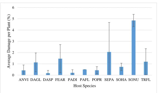
Figure 17. Comparison of damage between species, with standard error bars. The differences in damage between the plant species are not statistically significant.
Figure 18. Comparison of damage between tribes, with standard error bars. The differences in damage between the plant tribes are not statistically significant.
0 1 2 3 4 5 6
ANVI DAGL DASP FEAR PADI PAFL POPR SEPA SOHA SONU TRFL
A
v
er
ag
e
Dam
ag
e
p
er
P
lan
t (
%)
Host Species
0 0.5 1 1.5 2 2.5 3 3.5 4
A
v
er
ag
e
Dam
ag
e
p
er
P
lan
t (
%)
Figure 19. Comparison of damage between plants of different origin, with standard error bars. The differences in damage between the plant origins are not statistically significant.
Figure 20. Comparison of damage between plants with different photosynthetic pathways, with standard error bars. The differences in damage between the plant photosynthetic pathways are not statistically significant.
0 0.5 1 1.5 2 2.5 3 3.5
Americas Eurasia
A
v
er
ag
e
Dam
ag
e
p
er
P
lan
t (
%)
Origin
0 0.5 1 1.5 2 2.5 3 3.5
C3 C4
A
v
er
ag
e
Dam
ag
e
p
er
P
lan
t (
%)
Figure 21. Comparison between damage and photosynthesis rate, with linear regression. Photosynthesis rate does not significantly contribute to the variation in damage. The equation for linear regression for this model is y = -0.0005x + 1.0787, with R² = 2E-06.
Figure 22. Comparison between damage and leaf growth rate, with linear regression. Leaf growth rate does not significantly contribute to the variation in damage. The equation for linear regression for this model is y = 0.036x + 1.0292, with R² = 0.0008.
0 1 2 3 4 5 6
0.000 2.000 4.000 6.000 8.000 10.000 12.000 14.000 16.000 18.000
A
v
er
ag
e
Dam
ag
e
p
er
P
lan
t (
%)
Photosynthesis Rate (PN)
0 1 2 3 4 5 6
0.000 1.000 2.000 3.000 4.000 5.000
A
v
er
ag
e
Dam
ag
e
p
er
P
lan
t (
%)
Figure 23. Comparison between damage and LMA, with linear regression. LMA does not significantly contribute to the variation in damage. The equation for linear regression for this model is y = 23.878x + 1.0051, with R² = 0.0003.
Field Experiment by Tribe
Figure 24. Comparison between damage and photosynthesis rate, separated by tribe, with linear regressions. The equation for the Andropogoneae linear regression for this model is y = 0.0914x + 0.8821, with R² = 0.0469. The equation for the Poeae linear regression for this model is y = -0.0941x + 1.6919, with R² = 0.1008. The equation for the Danthonieae linear regression for this model is y = -0.0076x + 0.2315, with R² = 0.0196. The equation for the Paniceae linear regression for this model is y = -0.5948x + 4.5161, with R² = 0.4359. The equation for the Cynodoneae linear regression for this model is y = 0.2161x - 0.416, with R² = 0.8971.
0 1 2 3 4 5 6
1.0E-03 1.5E-03 2.0E-03 2.5E-03 3.0E-03 3.5E-03 4.0E-03 4.5E-03 5.0E-03 5.5E-03
A v er ag e Dam ag e p er P lan t ( %)
Leaf Mass per Area (g/cm2)
0 1 2 3 4 5 6
0.000 5.000 10.000 15.000 20.000
Me an Dam ag e p er P lan t ( %)
Photosynthesis Rate (PN)
Figure 25. Comparison between damage and LMA, separated by tribe, with linear regressions. The equation for the Andropogoneae linear regression for this model is y = 70.203x + 1.2949, with R² = 0.0017. The equation for the Poeae linear regression for this model is y = 602.14x - 0.4256, with R² = 0.3958. The equation for the Danthonieae linear regression for this model is y = -425.16x + 1.8587, with R² = 0.2995. The equation for the Paniceae linear regression for this model is y = -1363.5x + 4.7544, with R² = 0.3584. The equation for the Cynodoneae linear regression for this model is y = -1385.6x + 5.0873, with R² = 0.8118.
Figure 26. Comparison between damage and leaf growth rate, separated by tribe, with linear regressions. The equation for the Andropogoneae linear regression for this model is y = -0.3596x + 2.0607, with R² = 0.0379. The equation for the Poeae linear regression for this model is y = -0.0197x + 1.1851, with R² = 0.0006. The equation for the Danthonieae linear regression for this model is y = 0.1652x + 0.0251, with R² = 0.4516. The equation for the Paniceae linear regression for this model is y = 0.5151x + 0.2843, with R² = 0.1054. The equation for the Cynodoneae linear regression for this model is y = -1.6515x + 3.1086, with R² = 0.7358.
0 1 2 3 4 5 6
1.0E-03 2.0E-03 3.0E-03 4.0E-03 5.0E-03 6.0E-03
Me an Dam ag e p er P lan t ( %)
Leaf Mass per Area (g/cm2)
Andropogoneae Poeae Danthonieae Paniceae Cynodonteae Linear (Andropogoneae) Linear (Poeae) Linear (Danthonieae) Linear (Paniceae) Linear (Cynodonteae) 0 1 2 3 4 5 6
0.000 1.000 2.000 3.000 4.000 5.000
Me an Dam ag e p er P lan t ( %)
Leaf Growth Rate (cm/day)
Field Experiment by Origin
Figure 27. Comparison between damage and photosynthesis rate, separated by origin, with linear regressions. The equation for the Americas linear regression for this model is y = 0.0756x + 0.5647, with R² = 0.0219. The equation for the Eurasia linear regression for this model is y = -0.0589x + 1.4419, with R² = 0.0662.
Figure 28. Comparison between damage and LMA, separated by origin, with linear regressions. The equation for the Americas linear regression for this model is y = -859.41x + 3.939, with R² = 0.1428. The equation for the Eurasia linear regression for this model is y = 569.72x - 0.3058, with R² = 0.3999. This model statistically significant (Multiple R² = 0.2128, p = 0.01381).
0 1 2 3 4 5 6
0.000 5.000 10.000 15.000 20.000
Me
an
Dam
ag
e
p
er
P
lan
t (
%)
Photosynthesis Rate (PN)
Americas
Eurasia
Linear (Americas)
Linear (Eurasia)
0 1 2 3 4 5 6
1.0E-03 2.0E-03 3.0E-03 4.0E-03 5.0E-03 6.0E-03
Me
an
Dam
ag
e
p
er
P
lan
t (
%)
Leaf Mass per Area (g/cm2)
Americas
Eurasia
Linear (Americas)
Field Experiment by Photosynthetic Pathway
Figure 30. Comparison between damage and photosynthesis rate, separated by photosynthetic pathway, with linear regressions. The equation for the C3 linear regression for this model is y = -0.0909x + 1.499, with R² = 0.1128. The equation for the C4 linear regression for this model is y = 0.0738x + 0.6908, with R² = 0.0268.
0 1 2 3 4 5 6
0.000 1.000 2.000 3.000 4.000 5.000
Me
an
Dam
ag
e
p
er
P
lan
t (
%)
Leaf Growth (cm/day)
Americas
Eurasia
Linear (Americas)
Linear (Eurasia)
0 1 2 3 4 5 6
0.000 5.000 10.000 15.000 20.000
Me
an
Dam
ag
e
p
er
P
lan
t (
%)
Photosynthesis Rate (PN)
C3
C4
Linear (C3)
Linear (C4)
Figure 31. Comparison between damage and LMA, separated by photosynthetic pathway, with linear regressions. The equation for the C3 linear regression for this model is y = 260.99x + 0.1816, with R² = 0.083. The equation for the C4 linear regression for this model is y = -295.73x + 2.0621, with R² = 0.0255.
Figure 32. Comparison between damage and leaf growth rate, separated by photosynthetic pathway, with linear regressions. The equation for the C3 linear regression for this model is y = 0.0597x + 0.8661, with R² = 0.0052. The equation for the C4 linear regression for this model is y = 0.0077x + 1.1778, with RR² = 2E-05.
0 1 2 3 4 5 6
1.0E-03 2.0E-03 3.0E-03 4.0E-03 5.0E-03 6.0E-03
Me
an
Dam
ag
e
p
er
P
lan
t (
%)
Leaf Mass per Area (g/cm2)
C3
C4
Linear (C3)
Linear (C4)
0 1 2 3 4 5 6
0.000 1.000 2.000 3.000 4.000 5.000
Me
an
Dam
ag
e
p
er
P
lan
t (
%)
Leaf Growth Rate (cm/day)
C3
C4
Linear (C3)
ACKNOWLEDGEMENTS
REFERENCES
Cuomo, C., et al. (2007). “The Fusarium graminearum Genome Reveals a Link Between Localized Polymorphism and Pathogen Specialization”. Science 317 (5843), 1400-1402. Davidson, A. M., Jennions, M., & Nicotra, A. B. (2011). “Do invasivespecies show higher
phenotypic plasticity than native species and, if so, is it adaptive? A meta-analysis”. Ecology Letters 14, 419-431.
Davis, M.A., Grime, J.P., Thompson, K. (2000). "Fluctuating resources in plant communities: A general theory of invasibility". Journal of Ecology 88 (3), 528–534.
Gilbert, G., Webb, C. (2007). “Phylogenetic signal in plant pathogen–host range”. PNAS 104
(12), 4979–4983.
Kolar, C.S., Lodge, D.M. (2001). "Progress in invasion biology: predicting invaders". Trends in Ecology & Evolution 16 (4), 199–204.
Kumar, K., Xi, K., Turkington, T. K., Tekauz, A., Helm, J. H., Tewari, J. P. (2011). “Evaluation of a detached leaf assay to measure Fusarium head blight resistance components in barley”. Canadian Journal of Plant Pathology 33 (3), 364-374.
Montserrat, V., Maron, John L., & Marco, Laia. (2005). “Evidence for the Enemy Release Hypothesis in Hypericum perforatum”. Oecologia 142 (3), 474-479.