i
The Student Loan Debt Market:
The role of federal student loan allocation on undergraduate student default
rates
Erin Alyse Rowe
An honors thesis submitted to the faculty of the Kenan-Flagler Business School at the University of North Carolina at Chapel Hill
Chapel Hill 2014
ii ABSTRACT
Erin A. Rowe
The role of federal student loan allocation on undergraduate student repayment struggles (Under direction of Professor Bin Hu)
This study examines the effectiveness of federal student loan allocation and its role in student loan default rates. The loan allocation method is represented by program loan limits imposed by Congress. In addition to program loan limits, the study considers other educational and economic institutional drivers that education research has been linked to student loan default rates. The relationship between loan limits, other variables, and default rates is tested through a
iii TABLE OF CONTENTS
ABSTRACT ... II
LIST OF FIGURES ... VI
CHAPTER ONE: INTRODUCTION ... 1
FEDERAL STUDENT AID COMPONENTS AND ALLOCATION PROCESS ... 4
Definitions under Student Assistance ... 5
Evaluation of Student Aid Types ... 10
Student Loan Process ... 10
Evaluation of Student Loan Process ... 13
THE NATURE OF STUDY ... 14
CHAPTER TWO: LITERATURE REVIEW ... 15
RELEVANCE OF STUDENT LOAN PROGRAM MAXIMUMS ... 15
HISTORY OF FEDERAL STUDENT LOAN PROGRAM MAXIMUMS ... 17
CONTROVERSY OF PROGRAM LOAN LIMITS ... 20
Benefits of Loan Limits ... 20
Disadvantages of Loan Limits ... 21
Loan Limit Literature Implications... 23
IMPACT OF STUDENT LOAN DEFAULT... 23
POTENTIAL CAUSES OF DEFAULT RATES ... 27
Individual Characteristics ... 27
Cost of Attendance ... 28
Number of Loan Recipients ... 29
Number of Grant Recipients ... 30
iv
Significance of Default Literature ... 31
CHAPTER THREE: METHODOLOGY ... 32
DATA SELECTION APPROACH ... 32
RESEARCH DESIGN AND DATA COLLECTION ... 33
DATA MEASUREMENT PROCESS:MULTIPLE REGRESSION ANALYSIS ... 34
RATIONALE FOR SELECTED VARIABLES ... 35
Two-Year Cohort Default Rates ... 35
Student Loan Limits ... 36
Other Educational Drivers ... 37
Economic Drivers ... 38
LIMITATIONS ... 40
CHAPTER FOUR: RESULTS ... 41
CHAPTER FIVE: ITERPRETATIONS OF RESULTS ... 51
QUESTION 1:TO WHAT EXTENT DOES FEDERAL LOAN ALLOCATION IMPACT STUDENT DEFAULT RATES? .. 51
QUESTION 2:IS LOAN ALLOCATION OR ANY OTHER INSTITUTIONAL FACTOR SIGNIFICANT CONTRIBUTORS TO STUDENT LOAN DEFAULT? ... 52
OTHER NOTABLE FINDINGS ... 53
CHAPTER SIX: DISCUSSION OF POLICY IMPLICATIONS ... 54
PRESIDENT OBAMA’S STUDENT LOAN REVISIONS ... 55
Paying for Performance ... 55
Promote Innovation and Competition ... 56
EVALUATION OF PRESIDENT OBAMA’S INDICATIVES ... 57
INCOME SHARE AGREEMENTS ... 58
EVALUATION OF INCOME SHARE AGREEMENTS ... 59
v
EVALUATION OF INCOME CONTINGENT LOANS ... 61
RESOLUTION OF ALTERNATIVES ... 62
CHAPTER SEVEN: CONCLUSION ... 63
PERSONAL REFLECTION ... 64
APPENDIX A: REGRESSION TABLES ... I
EXHIBITA1:PUBLIC SCHOOL MODEL DATA ... II EXHIBITA2:PUBLIC SCHOOL CORRELATION MATRICES ... III EXHIBITA3:PUBLIC SCHOOL REGRESSION RESULTS ... IV EXHIBITA4:PRIVATE SCHOOL MODEL DATA ... V EXHIBITA5:PRIVATE CORRELATION MATRICES ... VI EXHIBITA6:PRIVATE REGRESSION ANALYSIS ... VII
vi LIST OF FIGURES
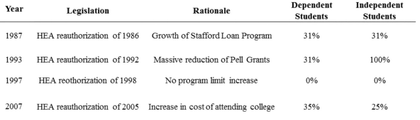
FIGURE 1PERCENT INCREASES OF PROGRAM MAXIMUM BY DEPENDENCY TYPE FROM HEA
REAUTHORIZATIONS... 18
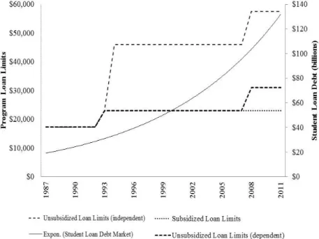
FIGURE 2THE RELATIONSHIP BETWEEN PROGRAM LIMITS AND STUDENT LOAN DEBT LEVEL ... 19
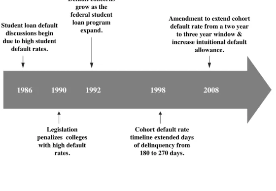
FIGURE 3THE PROGRESSION ON DEFAULT RATE POLICY ... 25
FIGURE 4TWO-YR.COHORT DEFAULT RATE AND AMOUNT ... 27
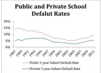
FIGURE 5PUBLIC AND PRIVATE SCHOOL DEFAULT RATES ... 36
FIGURE 6PUBLIC AND PRIVATE SCHOOL LOAN RECIPIENTS ... 38
FIGURE 7PUBLIC AND PRIVATE SCHOOL STATE AND GRANT AID RECIPIENTS ... 38
FIGURE 8FORRATIO FROM 1987-2011 ... 39
i
“When I entered college I was sold a lot of stories about how it was ok to take out loans every year because I would get a job that would pay them off. The only problem was that I was attending a private school that cost over $40,000 per year. I met my husband there and after we finished our undergraduate work, we went on to master's degree hoping to see the economy turn around. The only problem is that the economy has not turned around the way we need it to and we have built a combined total student debt of over $330,000 including interest. I am currently working out of field as a teacher making $30,000 a year and my husband is working part time. In a few months debt collectors will start calling for over $3,000 a month in student loan payments. The only problem is we only make $2800 a month after taxes and our other living expenses total approximately $2,200 a month. This means that we will be unable to pay over $2,400 a month in student debt. We don't own anything they can take from us so they will go after our cosigners. We can't find anyone who can help us. We have talked to debt consolidation agencies and no one can or will help us. We are drowning all because someone sold us up the river with a story about how great student loans were and how getting a college education would put us ahead of others. Where is this magical educational advantage that everyone likes to talk about because my husband has an MBA and is working as a security guard. We need help. How are ever supposed to make a life for ourselves? How are we ever supposed to own a home or have children when we make a tenth of what we owe in debt? We do take some responsibility for the situation we are in, but at the same time, what were our counselors and lenders thinking when they told a couple of 18 year old college freshman that it was ok to borrow $300,000? How can we possibly get out of
this?”
-- Christen Kauffman, Teacher from Florida
Christen Kauffman’s story represents one of427 first-hand accounts of student loan borrowers’ repayment struggles. She posted on The Project on StudentDebt’s web
forum1 to join the voices of other borrowers frustrated with their student loan debt load. Her story echoes the central theme of all other borrowers’ stories—inadequate level of
income to cover her student loan debt (“Voices”, 2014).
Christen, like other borrowers, blame many players for student loan debt. Players include Congress, the executive branch, colleges, and financial institutions. Congress sets
statutory standards on student aid eligibility standards, types, and amount through legislation, while the President establishes higher education initiatives and goals.
Meanwhile, the postsecondary institutions determine individual amounts of aid provided
2 to students that they received from the Education Department (ED) or a financial
institution (Taggart, 2010;; “Student Loans,” 2014). Because each of these three groups affects federal student loans, student loan borrowers also seek all players’ perspectives on higher education financing. The relationship between players is frustrating if borrowers’
investment in higher education backfires.
Higher education has become an “economic imperative” (Obama, 2011, para. 40)
for success in the U.S. President Obama has recognized the importance of higher education; and therefore, established higher education as a national priority (Obama, 2011). Alongside the President, studies from the ED, Sallie Mae, and the Institute for
College and Success, promote the necessity of higher education as well, linking higher education with higher future earnings (Baum, S., Ma, J., & Payea, K., 2013). As policy
makers and advocates share their perspectives on higher education with potential college students, more and more students buy into the justification to pursue postsecondary education. In Sallie Mae’s National Study, it affirms that over 70% of students attend
college because it is required for a desired occupation or necessary to earn a higher salary (How America Pays for College 2012, 2012).
While many preach the wonders of education, they fail to address how students and families can pay for the expensive investment. Student loans have become the most popular way for students to pay for a college education (How America Pays for College
2012, 2012; Baum, S., & Payea, K., 2013). However, the popularity is accompanied by a
$1 trillion student loan debt market (Chopra, 2012). Popular press, like Forbes or CFPB2
3
blogs, has labeled the increase in student loan borrowers with scary words like “bubble”
(Donlan, 2014, para.19) or “too big to fail” (Chopra, 2012, para. 2).
Dolan (2014), a writer for Forbes, applied the economic bubble analogy—the overinvestment in an asset that results in a devaluation of the asset—to the student loan
debt market. Dolan determines that as college tuition rises, the rate of return on a college degree decreases; discrediting the soundness of student loan industry because more
students default. Students who do not find employment needed to repay student loans are compared to debtors under sub-prime mortgages whose homes are worth less than what is owed to the bank. The difference between student loans and sub-prime mortgages is that
students can never get away from their bad debt.
Additionally, as students borrowed $117 billion in federal student loans in 2011,
Chopra, a blogger from the CFPB, deems it possibly “too big to fail” (Chopra, 2012, para. 2). The theory references financial institutions that are so large and interconnected that their failure would be detrimental to the entire economy. Thus, the government
should bail them out if the institutions were to collapse. Analogously, the student loan debt slows down borrowers’ ability to start a business, buy a home, or otherwise reinvest
in the economy. If the student debt market is too big to be self-sustainable, a bailout would manifest itself in debt forgiveness programs at the expense of tax payers.
The bubble and “too big to fail” postulates warn how detrimental student loans
can be on society. Because of the importance of higher education, the size of the student loan debt market, and the recent increase in student loan default, I first consider the
4
Federal Student Aid Components and Allocation Process
The Higher Education Act of 1965 (HEA’65) began federal student aid. Under the
HEA ’65 and future reauthorizations, Congress and ED defined student aid types and the
student loan process. This section first outlines the changes in the HEA and then
discusses the benefits and drawbacks of different federal aid types and the loan allocation process.
The History of Higher Education Student Assistance
The Higher Education Act of 1965 (HEA ’65) continued a pre-existing link
between policy and higher education financing. Public policy and higher education financing first became intertwined when President Lincoln signed the Morrill Act3 into
law in 1862 (Loss, 2012). Since establishing the Morrill Act, the government’s
involvement in higher education funding continued to increase through legislation like the GI Bill4 in 1944 and the National Defense Education Act of 19585 (Hannah, 1996).
Then, HEA ’65 “brought together a variety of [these] existing student aid programs
designed to meet earlier national education needs” (Hannah, 1996, p. 503).
Key amendments structured present higher education policy. Between 1965 and 1992, multiple amendments were made to HEA ’65 which included the introduction of
Sallie Mae and Pell grants. Throughout the next 30 years, amendments fluctuated
between tightening and loosening borrowing regulations, such as income caps, interest
3Morrill Act: Signed into law by President Lincoln, the Morrill Act of 1862 provided each state 30,000 acres of public land to encourage the establishment of higher education institutions to school people in agriculture, home economics, mechanical arts, and other professions.
4GI Bill: Signed into law by President Roosevelt, the Servicemen’s readjustment Act of 1944 (known as the GI Bill of Rights) gave veterans financial support to attend higher education institutions.
5 rates, and loan discernment (Hannah, 1996). In 1992, Congress reauthorized HEA which
Susan Hannah suggests shifted Title IV’s purpose from providing need-based educational financing assistance to broadening the student loan consumer base (Hannah, 1996). From 1992 to 2008, the number of Pell grant recipients remained small, denying the neediest
group of potential college students a federal financial cushion. On the other hand, student loan legislation allocated more money to a wider range of potential college students. In
2008, President Obama and Congress increased the number of grant recipients and attempted to include more financially needy students in the HEOA to refocus the purpose of financial aid (“Student Loans,” 2014).
While HEA ’65 includes six sections or “Titles,” this thesis focuses on the
amendments to “Title IV, Student Assistance,” from its inception to date. Title IV
outlined federal grants and scholarship opportunities, federally subsidized Stafford Loans, and work-study programs (Higher Education Act of 1965 [HEA ’65]). The following section details each type of financial aid.
Definitions under Student Assistance
Students pursuing postsecondary education can attain many types of financial assistance in the form of a gift, loan, or work-study. Federal and state governments as well as private institutions provide student assistance. Typically, federal loans have fixed
interest rates while private loans have variable interest rates (The Student Guide, 2010). Below are the most relevant types of student assistance along with benefits and
6
Federal Pell Grant (Pell grant): A Pell grant does not have to be repaid and is awarded to undergraduate students who demonstrate financial need, which is usually determined by the student’s family income. While Pell grants are ideal
for financially needy students, from a government perspective, it is the riskiest aid type because of the initial upfront cost with no explicit monetary payback. Hence, the federal government is investing in a student whose future impact on
the economy is unknown (Barrow, L., Brock, T., & Rouse, E. 2013).
Work-study Program (work-study): Work-study programs allow a student to
earn money to pay for his/her education. The government considers the student’s
financial need in awarding students participation in work-study programs by
providing funds to institutions to subsidize student wages. Work-study
encourages students to earn money for provided services. Although the federal
government incurs an upfront cost, student employees are contributing to the economy (Barrow, L., Brock, T., & Rouse, E. 2013). Work-study accounts for less than 1% of federal aid, a historically standard amount, meaning it impacts a
small percentage of aid recipients (Baum, S., & Payea, K., 2013).
Federal Perkins Loans (Perkins loans): A Perkins loan is lent by individual colleges to undergraduate or graduate students. Federal Perkins Loans are the optimal loan. The federal government provides colleges with limited funds to
provide a few of the neediest students subsidized loans at a lower interest rate. The loan also has an abbreviated repayment plan compared to other federal student loans and offers better cancellation previsions6. Since the government
7 makes less money on the loan, its benefits are not spread among much of the
borrower population, consistently accounting for less than 4% of borrower student aid (“Student Loans,” 2014;; Baum, S., & Payea, K., 2011).
William D. Ford Direct Stafford Loans (Direct Loans or Stafford loans): Direct
loans are lent directly from the ED to the student, rather than from a financial instruction originating the loan. The Direct Loan can be either subsidized or
unsubsidized. For a subsidized loan, the ED pays interest on the loan until the
student graduates from college provided the student demonstrates financial need.
For an unsubsidized loan, the student pays the accrued interest on the loan once he/she has graduated from college, and the student does not need to demonstrate financial need. Colleges determine the amount of aid an individual receives.
Direct Loans simplify the loan allocation process by making the postsecondary institution a one-stop-shop where the student receives loans and asks questions.
However, the student is unable to shop the loan offer because the loan is only provided by the ED (“Student Loan Basics,” 2014).
Direct PLUS Loans (PLUS Loans): PLUS Loans are unsubsidized direct loans
provided from the ED to graduate/professional students and parents of dependent
undergraduate students. While the ED does not require financial need, the borrower must display a good credit history. PLUS loans are beneficial because they allow parents to invest in their child’s future as well. Since PLUS loans
cannot be transferred to the student, it protects student borrowers from having larger debt loads due to their parents’ decision, although many students are held
8 It is also easier for the federal government to vet parent borrowers because they
have an existing credit history to be evaluated. A drawback to the additional borrowing option is that parents also may not realize Stafford loans have a lower interest rate, 3.86% versus 6.14%. Also, there are alternative methods for a parent
to borrow for their child that is tax deductible, such as home equity loans (“Student Loans,” 2014).
Direct Consolidation Loans (Consolidation Loans): Consolidation Loans allow
students to combine multiple federal student loans into one loan. However, PLUS
loans cannot be transferred to the student. Loan consolidation simplifies the loan process which helps financial management skills and provides students an opportunity to pay a lower interest rate on their loans. However, if borrowers are
not savvy in financial literacy, they may consolidate when it is not beneficial. For example, if the borrower has several loans with a varying range of interest rates,
it would be advantageous to accelerate the payment of the high interest loan rather than consolidate and pay more in the end (“Student Loans,” 2014).
Private Loans: Private Loans are issued from non-government institutions.
Private loans are unsubsidized and usually require the student to have a good line
of credit. Private loans cannot be consolidated with federal loans. Private loans give students an alternative method to finance higher education when federal student loans are not sufficient. On the other hand, private loans have higher
interest rates, less oversight, and less transparent payback plan. Also the student has to work with banks or other lending institutions rather than their college
9
Federal Family Education Loan Program (FFEL Loans): FFEL Loans
encompass Stafford Loans, PLUS Loans, and Consolidated Loans from private lenders rather than government institutions. FFELP Loans enlist multiple parties.
Similar to direct loans, the school determines financial eligibility. Then there is a lender, guarantor, servicer, collection agencies, and a secondary market. The lender is a private institution, like Sallie Mae. The guarantor, a non-profit
organization, works with the ED, lenders, services and schools to ensure students repay their loans. The servicer collects the loan payments and assists and answers
questions concerning students’ loans. The collection agency specializes in
delinquent/defaulted loans and is hired by lenders to recover loans. Lastly, the secondary market buys loans from lenders to provide capital for lenders to
originate the loans. The benefit to FFEL Loans is the power of choice. The frustration many students felt was the confusion in navigating multiple parties
(“Student Loan Basics,” 2014). FFEL Loans have not been offered since 2010 (“Student Loans,” 2014).
Each federal aid type could be advantageous for a certain borrower or parent. The key to maximizing the federal aid a student receives is his/her ability to navigate the choices. Overall, students receive Stafford loans when they apply for federal financial aid—
10 Evaluation of Student Aid Types
After considering the loan options, there are two problems with the current student loan structure. First, there are too many types of student aid (Dynarski & Scott-Clayton, 2013). Currently, the ED allows students to borrow from a variety of debt
instruments. Choice is preferred in a transparent market where the consumer fully understands his/her options. For student financial aid, each instrument has numerous
intricacies which the ED unfairly expects high school graduates to understand. I applaud the ED, along with President Obama and higher education advocacy groups who are working to provide clarity in the market through better financial aid counseling.
However, maintaining a laundry list of financial aid types is still worrisome. Second, the federal financial aid that is the best value for a student is misaligned with the aid that is
the best value for the lender, either the ED or private institutions. Namely, work-study and Perkins Loan programs account for 5% of all financial aid but provide students with the highest return on educational investment. However, other student loan types have
higher interest rates, costing students much more. Economically, in order for the ED to sustain a federal aid program, they have to charge students more; socially, the federal
government should also work to benefit borrowers.
Student Loan Process
A borrower, student or parent, must follow certain steps to obtain student
assistance, federal or private. To obtain federal assistance, the borrower outlines the cost
11 domestic loan, and thus the process parallels other loan processes (The Student Guide,
2010). Then after the borrower graduates, he/she follows a repayment plan.
To apply for federal student assistance, a student completes a series of steps. First, a student must submit a Free Application for Federal Student Aid (FAFSA) for the
government to determine the financial neediness of the student. FAFSA determines eligibility for grants, work-study, state aid, and loan type. After submitting the FAFSA,
the ED sends the student a Student Aid Report (SAR) with a summary of the FAFSA and Expected Family Contribution (EFC), which determines the eligibility for different student assistance programs. The SAR is sent to the postsecondary institutions that the
student has indicated on the FAFSA. The postsecondary institution determines eligibility and the amount based on a student’s financial need, the difference between EFC and
COA (The Student Guide, 2010). Next, a student receives an award letter outlining the student’s financial aid package which explains payment schedules and expense
breakdowns. Once accepting the loan, the student commits to the payment schedule and
the loan provider commits to the allotted amount7. Lastly, the student receives the money in two disbursements (“Smart about College”, 2011).
To qualify for any federal student aid, students have to meet specific basic requirements. Basic eligibility requirements to receive federal financial aid are:
Demonstration of financial need;
Proof of U.S. citizenship or non-citizenship eligibility;
A valid Social Security number;
Registration with the Selective Service (males only);
12 Showing of enrollment or acceptance for enrollment by an eligible degree
program;
Part-time enrollment to receive Direct Loans;
Maintenance of satisfactory academic progress;
A promise to spend aid for only educational purposes; and
Demonstration of a high school diploma or General Educational Development (GED) certificate (Smart about college, 2011).
These basic requirements have changed only slightly since 1965, except for the FAFSA report, which the government added through HEA ’92. Once the government decides that
the student meets the criteria, the government assesses financial need to determine federal
student aid allocation (The Student Guide, 2010).
After graduation, a borrower chooses one of the four types of repayment plans:
(1) standard repayment; (2) extended repayment; (3) graduated repayment; and (4) a percentage of income repayment. Also, a borrower is entitled to change repayment plans during the repayment period. A borrower under the standard repayment plan pays a fixed
monthly amount of the loan for up to 10 years. The extended monthly repayment plan copies the standard repayment plan except it allows borrowers 12 to 30 years to reduce
the size of repayment but increases the lifetime total amount paid. The graduated repayment plan begins with smaller monthly payments and increases every two years lasting 12 to 30 years.
Lastly, there are three plans that consider a borrower’s income. The income-contingent repayment plan pays a percentage of the borrower’s income and monthly
13 This is similar to the Income Sensitive Repayment plan offered to FFELP borrowers.
Income-Based Repayment caps monthly payments at a lower percentage of discretionary income instead of gross income (“Student loans”, 2014).
Evaluation of Student Loan Process
While the standardized student loan process connects a number of students with
financial aid, it is overly complex and inefficient. First, the FAFSA is a daunting
application which rivals a 1040 tax form in length. It takes approximately three hours to complete and is usually filled out incorrectly by students not familiar with the financial
aid process. The document should be streamlined to incorporate only unavailable information about a potential borrower (Dynarski and Scott-Clayton, 2013). The
FAFSA’s intimidation causes many students to miss aid opportunities. In 2007, 2.3
million students were not considered for Pell grant aid because they did not complete the FAFSA (Abernathy et al. (2013).
Second, the financial equation colleges use to determine aid eligibility and amount ineffectively evaluates students. While Direct PLUS borrowers have sufficient
credit history to be screened, the ED has less specific information for student borrowers (Abernathy et al., 2013). Dynarski and Scott-Clayton (2013) argue that the ED lacks structure in ranking student eligibility, resulting in the student aid agency incorrectly
identifying the types of aid, gifts, unsubsidized loans, subsidized loans, or a combination of any they award students. The equation also does not measure individual
14
The Nature of Study
The purpose of this thesis is to evaluate the effectiveness of the federal Stafford student loan allocation for undergraduate students. The role of Stafford loans is
interesting since they are taken on by the majority of loan recipients. As Dynarski and
Scott-Clayton (2013) highlight the inefficiency of the student loan process and borrowers, like Christen Kauffman relays distress in repaying her student loan amount, the study
tests whether the two are linked. Loan allocation is measured by means of federal loan limits, the maximum amount a student is about to borrow, and a student default rate reflect student’s problems repaying loans.
Since the ED locks individual student borrower information for privacy reasons, I use public aggregated data to determine if loan allocation or any other institutional
factors impact student loan default. From the study, I attempt answer two questions: 1. To what extent does student loan allocation impact student default rates? 2. Is loan allocation or any other institutional factor significant contributors
to student loan default?
If loan allocation or any other institutional factor is the driving factor of student loan
default, then ED can depress default through restructuring institutional characteristics, like the amount or types of aid offered. However, if institutional factors do not
significantly drive student loan default, the ED should create an alternate method of
screening potential borrowers based on their individual characteristics.
My study uses empirical analysis to determine the impact of federal loan limits
15 and other potential institutional factors. Through the literature review, I build the
foundation for my study by analyzing existing research and evaluating controversial findings. Next, I outline the methodology of my study to explain the process for selecting and measuring the data used in the empirical study. Then, I report the results of my
analysis and determine statistically significant and other relevant relationships. From my findings, I answer my two questions. Lastly, I describe three popular higher education
financing alternatives and conclude how loan allocation can be reformed.
CHAPTER TWO: LITERATURE REVIEW
This section discusses the literature surrounding student loan allocation, student
loan default rates, and other higher educational institutional factors. To begin, I describe the relevance of student loan program maximums in loan allocation. Second, I provide a condensed history of federal student loan program maximums and discuss the
controversy around them. Next, I describe the impact of student loan default. Lastly, I describe other potential institutional drivers of student loan default.
Relevance of Student Loan Program Maximums
Under the HEA ’65, Congress established program loan limits to regulate federal
loan allocation. The loan limits established the maximum amount colleges could provide to aid-eligible students. The loan limits are tailored to several characteristics, including
the type of student loan, the nature of the loan (i.e., whether it is subsidized or
16
(HEA ’65;; “Student loans,” 2014)8. Congress created annual and aggregate loan limits
(program maximums), which are defined below:
Annual loan limit: The annual loan limit specifies the maximum loan amount a
student can borrow depending on year or credit status when attending a higher education institution. The annual loan limit changes as a student transition from freshman to senior year.
Aggregate loan limit (program maximum): The program maximum is the largest
loan amount a student can borrow throughout his/her undergraduate career (“Student loans,” 2014).
Also, students can borrow up to the program maximum but may be constrained by
individual borrowing maximums set by postsecondary institutions according to student financial need and budget. Hence, the individual maximum ranges from zero to the
program maximum (Wei & Skomsvold, 2011). This thesis analysis uses program loan limits for two reasons: (1) they encapsulate all underlying annual loan limit changes and (2) program loan limits are positively correlated with individual limits (Historical Loan
Limits, 2014).
Program maximums show the changes in annual loan limits since Congress
increases the limits proportionally. Hence, program loan limits represent increases in the underlying years as well. When borrowers begin repayment, they pay interest on the total amount they borrowed, not on their different annual loans individually.
More importantly, program limits are positively correlated with individual limits. NCES reports published in 1995 and 2013, 65% of public and private postsecondary
institutions ranked increasing program limits as a reason to increase individual maximum
17 allocation when considering student financial need (Lewis & Westat, 1995; Snyder &
Dillow, 2013). Additionally, in Borrowing at the Maximum (2011), Christina Chang Wei and Paul Skomsvold note trends in student borrowing at the loan limits in 2011. Wei and Skomsvold highlighted the trend of student borrowing in relation to loan limits from the
1980s to 2008. The authors found that between 40-50% of borrowers have taken out the program’s maximum amount. Also, many reports, such as those authored by the
American Institutes for Research, use program maximums as the proxy of loan limit effects and amounts students borrow.
As the majority of students borrow at or near loan limits, program maximums
allow Congress and the executive branch to manage the expansion and consolidation of the student loan debt market. Thus, program loan limit legislation not only considers
student need but also depends on political initiatives.
History of Federal Student Loan Program Maximums
Congressional legislative action resulted in incremental increases to program and annual loan limits presented in Figure 1. Congress enacted the first loan limit increase
within the 1986 HEA reauthorization process. Under President Regan, 1986 legislation established a need test to determine student eligibility which limited borrowing to the minimum amount students needed. However, the legislation increased program loan
limits by 38% in order to ensure future loan program growth for both subsidized and unsubsidized loans limits. Regan began the transition from grant to loan based aid. By the
18 college, forcing students to become more reliant on federal loans. With a desire to cut
federal spending, policy makers—including President George H. W. Bush—abandoned initiatives to focus federal aid on Pell grants which shifted primary federal aid
beneficiaries from the lower-income students to middle- and upper-income students by
raising loan limits an additional 31% for dependent students and 100% for independent students (Cervantes et al., 2005). The official move from a grant to a loan centric
financial aid policy resulted in exponential growth in the number of students borrowing loans and the amount students were allowed to borrow (Hannah, 1996). During the HEA Reauthorization of 1998, President Clinton exhibited fiscal discipline by not raising
federal loan limits but did raise the Pell maximum (Cervantes et al., 2005). Then, in 2007, President Obama declared the purpose of federal aid was to help all students achieve
higher education. In turn, he drastically raised student loan limits—by 35% and 25% for dependent and independent students, respectively—and raised the Pell grant to
compensate for the cost of attending higher education (Scott, 2011).
Note: Adapted from“Student Loans,” (2014). FinAid. Retrieved from http://www.finaid.org/loans/
19 While Congress and the executive branch strived to increase financing for
students’ higher education in a cost-effective manner, the reauthorizations that grew program maximums propelled student loan debt levels. As shown in Figure 2, student loan debt levels are strongly correlated with program loan limits implying that students
take advantage of program limit increases. Policy makers should be conscious of this association to ensure debt levels do not escalate to dramatic levels.
Source: “Student Loans,” (2014). FinAid. Retrieved from http://www.finaid.org/loans/
20
Controversy of Program Loan Limits
Although three out of four reauthorizations increased student loan limits, there have been numerous debates surrounding the effectiveness of the legislation. Generally, Republican administrations try to direct federal aid away from costly grant aid to revenue
generating student loan programs. Democratic admirations have attempted to expand aid to include more lower-income students either through Pell grants or federal student loans.
In the following paragraphs, I describe both advantages and drawbacks of loan limits as outlined by key influencers—policy makers, politicalorganizations, and academia.
Benefits of Loan Limits
Policy makers, much like Congress; certain political organizations, like the New America Foundation (NAF); and academia applaud the role of loan limits. The
Government Accountability Office (GAO), Congress’ auditing arm, endorses student
loan limits as a uniform method to regulate student borrowing. The GAO cites increased enrollment and borrowing numbers for full-time college programs to praise Congress for
successfully accomplishing two initiatives through student loan limits increases: (1) minimizing excessive student loan debt per borrower and (2) enabling students to finance their education through increased access to capital (Scott, 2011).
Political organizations, such as the New America Foundation9 (NAF), also voice supporting viewpoints on loan limits. The non-partisan organization explains that loan
limits control student borrowing and inhibit students from overborrowing. However, NAF concedes that loan limits are not the only avenue for the federal government or
21 colleges to monitor students’ accumulation of student loans. With limits, NAF proclaims
that colleges need to do a better job providing a multi-year price schedule, transparent financial need, and cost-of-attendance calculation to their students.
In the Journal of Economic Perspective, Avery and Turner (2012) claim that
capital availability, especially through student loans, is imperative to encourage students to invest in higher education. In addition, the authors encourage loan limit increases
because of the increased cost of attending higher education. Many other researchers substantiate Avery and Turner’s claim by pointing to the positive correlation between the
increase in access to capital—through loan limit upticks—and the increase in student
enrollment (Akyol & Athreya, 2005; Garriga & Keightley, 2007).
Disadvantages of Loan Limits
While some policy makers, political organizations, and some academics champion loan limits, others claim loan limits are an ineffective tool in managing the
amount students borrow. To start, President Obama has taken an active role in higher education and how students pay for it. The President has recently denounced the
successfulness of the current loan-allocation process. While President Obama views student loans as an avenue to increase college enrollment numbers, he highlights how current program limits do not match the quality of the postsecondary institution. Hence,
he states that student borrowing is reinforcing the bloated debt total and high student loan default rates. Thus, while the legislative and executive arms of government are aligned in
22 Within academia, opponents of loan limits disfavor randomly crafted loan limits
and unproductive individual student loan allocation. In research under the Federal Reserve Bank of St. Louis, Garriga and Keighley (2007) support the idea of capped borrowing but argue that loan limits come up short because they are arbitrarily created
and not indexed according to the cost of attendance increases or changes in inflation. Through their study of education policy, Garriga and Keighley assert that students are not
receiving the amount of aid they actually need. They further assert that loan limit increases should better track financial-need changes of students.
Additionally, some in academia worry that loan limits unsuccessfully tailor
individual loan amounts to students. In the Economics of Education Review, Hansen and Rhodes (1988) voice concern over the government haphazardly allocating extra capital
without understanding undergraduate borrowers. Through a study of borrowers with varying amounts of debt after the HEA reauthorization of 1986, Hansen and Rhodes determined that loan limit increases could amplify the amount borrowed by risk-prone
undergraduates who are uncertain of future earnings. Because student loans are uncollateralized, their research revealed the challenges faced by lenders, such as the
federal government and commercial banks, in appropriately vetting borrowers to determine risk appetite and reliability to pay back the loan (Hansen & Rhodes, 1988, Garriga & Keightley, 2007). Although Avery and Turner (2012) acknowledge loan limits
23 Loan Limit Literature Implications
Since 1992, loan limit legislation has wrestled with promoting college enrollment and mitigating excess borrowing. At inception, the HEA ‘65 established federal student loans to help low-income students to pay for college and created program loan limits to
keep that fraction of students from overborrowing. As the1992 reauthorization expanded program limits and borrower eligibility requirements, it became harder for Congress, the
ED, and colleges to predict perfect individual borrowing amounts because the student loan market and college landscape changed. In the student loan market, a greater number of diverse students are involved in the process, and cost of attending college surpassed
predictions. Hence, as shown by Hanson and Rhodes (1988); Garriga and Keightley (2007); Avery and Turner (2012), it is difficult to subjectively classify current loan
allocation method as good—because it is statistically shown to increase college
enrollment—or bad—because it allows Congress to arbitrarily distribute debt to students.
Impact of Student Loan Default
A student enters default if he/she fails to repay a federal student loan according to
the terms agreed to in the promissory note. As a general rule, a student has defaulted on student loan after 270 days of a missed payment10. If a borrower defaults on a student loan that is owned by ED, the borrower faces the following consequences: loan balance
due in full; loan collection fees; 15% deduction out of his/her paycheck; Social Security, disability income, and state and federal tax refunds taken; ineligibility for federal aid; and
ruined credit score. The borrower recovers from default by repaying the loan in full,
24
entering a loan rehabilitation program, or consolidating out of default (“Managing
Default,” 2014).
Annual default rates are measured by the official two-year cohort default rate (cohort default rate). The cohort default rate is the aggregated number of borrowers in
default who entered repayment on a certain Direct Loan or FFEL Loan two years prior. For example, the fiscal year (FY) 2011 cohort rates were released in 2013. To expand
payback period window, the HEOA of 2007 requires the ED to also calculate and report three-year cohort default rates beginning in 2009 (“Two-year Official Cohort Default Rates for School," 2013). By accounting for an additional payback year, the policy
change better reflects the reality of student prepayment problems.
Congress crafts student loan default policy by making incremental changes to the
HEA.Figure 3 presents the historic events that impacted default loan policy. First, during the 1986 reauthorization of HEA, student loan default rates became a recurring topic. Because student loan default rates were obscenely high, over 20%, Congress planned to
enact federal legislation that penalized colleges with high default rates (Gross et al., 2009). Then, beginning in 1990, the government declared colleges with student default
rates greater than 25% over three years or over 40% in one year ineligible to participate in federal student loan programs. The legislation ensured college accountability for student default behavior (Volkwein & Szelest, 1995). However, Congress’ concerns grew
after the expansion of student loans in the 1992 reauthorization. In 1998, Congress extended the amount of days a student could miss a payment from 180 days to 270 days.
(D-25 NY) and Raul Grijalya (D-AZ) expressed skepticism about default calculation11. In
response, Congress’ 2008 reauthorization act further extended the default calculation window to three years.
While changes in the HEA continue to increase college’s accountability for
default rates, Congress’ default rate caps place little pressure on most colleges. For example, less than 2% of colleges surpassed the student loan threshold while 10% of
student borrowers went into default (“Default Management,” 2013). Hence, the majority of colleges are unaffected by Congressional sanctions but are more likely to help students overborrow.
The Progression on Default Rate Policy
11Timothy Bishop (D-NY) and Raul Grijalya (D-AZ) introduced the amendment encompassed in the HEOA that extends the default window calculation to three years.
1986 1990 1992 1998 2008 Student loan default
discussions begin due to high student
default rates.
Legislation penalizes colleges
with high default rates.
Default concerns grow as the federal student
loan program expand.
Cohort default rate timeline extended days
of delinquency from 180 to 270 days.
Amendment to extend cohort default rate from a two year
to three year window & increase intuitional default
26 Student loan default has a high social cost to policymakers and students. On the
students’ side, student loan default can trap students because they cannot declare bankruptcy and abandon their debt. Hira et al. (2000) found that once students incur student loans, they are reluctant to invest in the economy through homes, cars, or credit
cards purchases because they fear entering default. Forbes writer Halah Touryalai affirms her own belief that student loan debt inhibits economic growth. Touryalai relays quote
from CFPB Director Richard Cordray discussing the inability for borrowers to take on other loans because of student loan debt and lack of credit (2014).
On the policy makers’ side, student loan default affirms misallocation of federal
loans. Policy makers and academia largely measure productivity of federal student loan programs by default rates of student loans (Gross et al., 2009). Over time, two-year
cohort default rates and default amounts are lower than they were during the late 1980s, but have recently increased since the Great Recession, as seen in Figure 4. Both policy makers and academia have voiced concern over the sharp increase in student loan default
amounts that is up 111% since 2007 (Two-Year Official Cohort Default Rate, 2013). Throughout the last five years, policy influencers have attempted to better understand
27
Figure 4 Two-yr. Cohort Default Rate and Amount
Note: Adapted from “Baum, S., & Payea, K. (2013). Trends in student aid: 2013.”
Potential Causes of Default Rates
In addition to loan limits, education research has isolated potential drivers that
impact student loan default. One driver is the individual borrower characteristics. The other five drivers are related to institutional factors: (1) higher education cost of
attendance; (2) number of loan recipients; (3) number of Pell Grant aid recipients; (4) the
economy’s view of debt;; and (5) the state of the economy (Goss et al., 2009;; Dynarski &
Scott-Clayton, 2013).
Individual Characteristics
Academia has released extensive research on the role of student borrower
characteristics and background. The characteristics include: age, race, gender, and family socioeconomic standing. Research findings are closely aligned regarding the impact of
$0 $100,000 $200,000 $300,000 $400,000 $500,000 $600,000 0% 5% 10% 15% 20% 25% 19 87 19 89 19 91 19 93 19 95 19 97 19 99 20 01 20 03 20 05 20 07 20 09 20 11 2 -y ea r Co ho rt Def a ult T o ta l 2 -y ea r Co ho rt Def a ult Ra te Cohort Year
28 each characteristic on the chance of default. Almost all research positively correlates a
student’s age with chance of default, often citing causes such as greater financial
obligations and less external monetary support (Gross et al., 2009; Choy & Li, 2006). Research on the borrower’s race concludes that borrower’s ethnicity is the greatest
predictor of default. Students of color, especially African Americans, have a greater probability of default than their Caucasian peers. Contrastingly, gender appears to have
little correlation with probability of default. Lastly, studies on the borrower’s family’s
socioeconomic standing suggest that students of higher income families are less likely to default because of a familial financial safety net. Thus, empirical research largely agrees
on how changes in borrower characteristics affect borrowers’ likeliness of default.
Financial planning can also play a role in the borrower’s likeliness of default
(Gross et al., 2009). Gross et al. (2009) cited Dynarski’s (1994) previous studies to validate the role of money management in the probability of student loan default. Sallie Mae (2012), Volkwin and Szelst (1995), and other studies agree with Dynarski’s (1994)
perspective on the importance of money management skills, especially as student
borrower debt expands into other consumer debt types (e.g. credit cards, auto loans, etc.).
Other types of consumer loan debt, particularly credit card debt, gain popularity as students attend college, indicated by the 60% of college seniors who owned a credit card in 2012, up 4% since 2011 (Sallie Mae, 2012).
Cost of Attendance
The cost of attending college has increased overtime, forcing students to invest
29 to help students surmount the cost threshold. Congress has increased loan limits in order
to match college cost increases. The ED works to educate students on loan opportunities and helps them complete their FAFSA applications (“Student Loans,” 2014).
Additionally, students have responded to upswings in college cost of attendance by
taking on more debt. Gross, Cekic, Hossler, and Hillman (2009) as well as Avery and Turner (2012) agree students’ responses to increased tuition fees have propelled them
into default.
Number of Loan Recipients
Researchers argue that the number of student aid recipients either increase or decrease default rates. In the Review of Higher Education, Hillman (2014) reports
increased popularity of higher education, coupled with federal and state efforts to increase college completion programs, expands the number of aid-reliant students. Hillman notes that the growth in the borrower population results in more students unable
to repay greater loan amounts. Hannah (1996) supported this notion years earlier when evaluating the inclusion of merit-based scholarships after the HEA Reauthorization Act
in 1992. Hannah found dangers in expanding the number of loan recipients because more students unaware of their future earnings were included in the loan pool which increased default rates. Dynarski and Scott-Clayton (2013) add that increasing the volume of
students unnecessarily receiving aid has caused the student loan debt total to bloat to unreasonably large levels.
30 who are not in the lower class and qualify for aid are more likely to repay their debt.
Thus, more borrowers lessen the riskiness of the pool of potential defaulters.
Number of Grant Recipients
Since 1965, policy makers and academia have conducted substantial research around federal grant aid. Keane summarizes the findings that suggest low income
students need grant support to get over the college cost threshold, and the decrease of grant aid recipients increase these students’ chances of default (2002). Hillman (2014) argues that the decrease in grant funding has increased student reliability regarding
student loans, thereby increasing the pool of potential defaulters. Interestingly, Hillman reports that students with higher amounts of grant aid have a greater chance of defaulting
because the neediest have the least amount of external support—family, friends, or otherwise— to finance student loans.
The Economy
The state of the economy also plays an influential role in determining a student’s
likelihood of default. During a recession, for example, the amount of money students have to repay loans are greatly constricted. The Economic Policy Institute reports that students who graduated during the Great Recession struggled more with repaying their
student loans (Shierholz, H. Wething, H. & Sabadish, N., 2012). They argue that not only are students’ financial resources constrained, but their possible support systems –family
31
unemployment increases a student’s odds of defaulting since job loss negatively impacts
financial resources used to pay student loan debt.
Additionally, student loan debt is only one type of household debt. Other
household debt includes car loans, credit card debt, and mortgages. As the economy goes
through peaks and troughs, household comfort for managing debt varies. During recessions, at times, households choose to pay off some debt over others. For example,
during the economic downturns, some people choose to pay off their car loans rather than their mortgage payment (Flint, 1997). Hence, the level of comfort the economy has with managing debt can indirectly impact student loan default rates.
Significance of Default Literature
Research has placed varying weights on the six variables to suggest which are more important in predicting student loan default. While much research sites the individual’s characteristics as the most relevant driver of student default (Gross et. al,
2009; Flint, 1997), the other institutional drivers play a role in students’ ability to pay back loans. Similarly to loan limits, it is difficult for Congress, the President, or academia
32
CHAPTER THREE: METHODOLOGY
In this section, I explain the steps in my data collection and analysis that lead to
my final results, the isolated impact of student loan borrowing limits on two-year cohort default rate. First, I describe my data selection approach. Second, I summarize my
research design and data collection. Next, I explain my data measurement process, multi-variable regression analysis. Then, I provide rationale for the multi-variables I use to determine the relationship between student loan limits and student default rates. Lastly, I reference
potential limitations of my research design.
Data Selection Approach
In my data selection approach, I delineate terminology, specify my study’s
timeframe, and distinguish participants’ profiles. To start, I narrow the focus of higher
education institutions as an establishment that offers post-secondary education to undergraduate or graduate student. Within higher education institutions, I only
concentrate on public and private schools. My definition of a public school is a state funded higher education institution built on a four-year program. Similarly, my definition
of a private school is a not-for-profit higher education institution built on a four-year program. Because of incomplete for-profit, higher education institutions data, I only focus on not-for-profit higher education institutions that educate 88% of post-secondary
students (NCES, 2012).
My data has a timeframe constraint to accommodate the student loan default rate
33
1987 cohort (“Student loans,” 2014). Thus, the study’s timeline begins in 1987 when
Congress encouraged institutions to refocus on providing affordable education to students. The study ends in 2011, the most recent cohort default rate released. The data collection timeline was not constrained by loan limits because the ED oversaw allocated
Stafford loans since inception (“Student loans,” 2014). Lastly, for the purpose of this
study, I tailor my analysis to the aid-eligible undergraduate population attending either
public or private schools.
Research Design and Data Collection
My research design aims to correlate loan limits and other variables to default rates. To begin my study, I collect data samples which academics postulate impact the
likelihood of students defaulting on their loans. Because I am studying and comparing the isolated impact of loan limits on public and private schools separately, I created a public school regression model and private school regression model. The two models allow me
to separate and compare the characteristics of students who attend either institution. The models measure identical variables with numbers stemming from public or private
instructions. I, then, compare the strength of the association between the dependent variable, cohort default rates, and the range of independent variables, namely student loan limits, to determine impactful drivers (Kleinbaum, Kupper, & Muller, 1988).
After considering the major drivers of student loan default rates, I compiled data through a range of public government sources. Any data related to higher education
34 Innovation as well as FinAid. The studies include reports from NCES and the
Information for Financial Aid Professionals (IFAP). The offices and studies have surveyed, aggregated, and updated facts/statistics about higher education since HEA indoctrination. Hence, they are the primary sources of other educational studies, such as
the Project on Student Debt, validating data accuracy. Moreover, for economic data I utilize reports from the Bureau of Economic Analysis, the Bureau of Labor Statistics, and
the Federal Reserve Board. Lastly, I note correlations between historical cohort default rates and other variables from the highlighted data the model to empirically report the role of loan limits on default rates.
Data Measurement Process: Multiple Regression Analysis
I use multi-variable regression analysis because it is the optimal analysis tool to evaluate the relationships between variables both quantitatively and qualitatively. After selecting and classifying my independent and dependent variables, I run multiple
regressions and analyze the significance of coefficients. I run correlation tables to ensure no independent variable measurements overlap and skew results (Kleinbaum, Kupper, &
Muller, 1988).
To analyze the data, I apply industry standards to determine the significance of a regression statistic. I use a .05 level of significance. Correlations between variables
should be less than .7, shown in Appendix A (Kleinbaum, Kupper, & Muller, 1988). For the public school and private school regressions, I evaluate the models’ based
35
Rationale for Selected Variables
The public and private school models consider identical dependent and independent variables. The two-year cohort default rate is the dependent variable,
meaning its outcome is measured against other drivers. The independent variables include
loan limits and four other drivers of default rates highlighted by academia. The
independent variables are grouped into either educational drivers or economic drivers.
The educational drivers include amount of public/private loan recipients and amount of private/public Pell Grant aid recipients. The economic drivers include the Financial Obligations Ratio and unemployment rates. These specific drivers are chosen by
considering two integral concepts: (1) variable representation within another variable and (2) level of variable significance. In this section, I describe the rational and computation
of the dependent variable, two-year cohort default rates as well as the independent variables, loan limits, other educational drivers, and economic drivers.
Two-Year Cohort Default Rates
ED’s archived default rate data sheets provided individual default rates for all
U.S. higher education institutions. I compile the two-year cohort rates by separately averaging all U.S. public and private school two-year cohort default rates. While three-year cohort default rates better encapsulate borrowers’ likelihood of default, I use two
-year default rates over the three--year due to lack of historical three--year default rate data (“Default Management,” 2013). Thus, two-year cohort default rates are the most
36
(“Student Loan Basics,” 2014). Figure 5 shows the changes in public and private school
default rates.
Figure 5 Public and Private School Default Rates
Note: Adapted from “Archive Two-Year Default Rates. Department of Education.”
Student Loan Limits
FinAid provides annual and aggregate student loan limits by type (subsidized or unsubsidized) and student dependency status. Since independent and dependent students qualify for different loan amounts, I standardize loan limits by applying weights based on
yearly dependency proportion breakdowns to the aggregate loan limit amounts. Additionally, Congress establishes loan limits separately from higher education
institution type, meaning loan limits are the same for the public school and private school model.
Variations in program loan limits also explain variation in individual loan limits
and college cost of attendance. Hence, individual loan limit amounts are not included in the model because individual amount variation is encapsulated in loan limit changes. The
37 (2) colleges use program limits increases to construct individual loan limits. Thus, the
program loan limit driver is more relevant to the study. Cost of attendance is not included in the model because Congress aims to construct program loan limits alongside increases in cost of attendance which causes the variables to have high collinearity which
negatively impacts the model. Changes in loan limit are shown in Figure 1.
Other Educational Drivers
Academia highlights other trends in higher education that could affect a student’s
chance of repayment: the growth of student loan recipients and the decrease of grant aid
(Gross et. al, 2009; Hillman, 2014). To test other educational trends, I collected the historical data from the NCES for amount of loan recipients as well as amount of Pell
grant and state grant recipients (Snyder, Dillow, & Hoffman, 2009). I normalize both variables by using the ratio of number of public/private recipients to number
public/private enrollment numbers each year. Furthermore, I solely use the number of
Pell and state grant recipients because the amount per recipient remains constant year over year. Figure 6 and 7 shows the changes in public and private school loan and grant
38
Figure 6 Public and Private School Loan Recipients
Note: Adapted from “Baum, S., & Payea, K. (2013). Trends in student aid: 2013.”
Figure 7 Public and Private School State and Grant Aid Recipients
Note: Adapted from “Baum, S., & Payea, K. (2013). Trends in student aid: 2013.”
Economic Drivers
The state of the employment economy impacts any debt borrower’s ability to
repay loans. I account for changes in the economy through multiple drivers. First, I 0%
20% 40% 60% 80% 100%
Public and Private School State
and Grant Aid Recipients
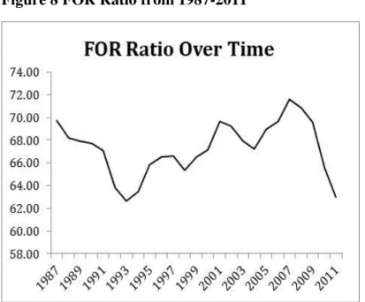
39 consider the financial obligations ratio (FOR) to account for consumers’ comfort with
debt. FOR estimates the ratio of household debt payment to disposable income and other financial obligations, such as automobile lease payments (Household Debt Service and Financial Obligations Ratios,” 2013). Second, I used unemployment reported by the
Census Bureau because academia has largely associated unemployment rates with likelihood of default because students have capital constraints (Woo, 2002). FOR Ratio
and unemployment rates over time is shown in Figure 8 and Figure 9.
Figure 8 FOR Ratio from 1987-2011
40
Figure 9 Unemployment Rate from 1987-2011
Note: Adapted from “US Census Bureau Data, 2010.”
Limitations
There are three possible limitations to my study that could influence the results. The first limitation is that I narrowed the definition of a higher education institution to
only not-for profit institutions. Knowing this, I will be aware of participant biases because of potential differing behaviors between students who attend for-profit higher
education institutions and students who attend not-for-profit institutions. However, because it is a small portion of the post-secondary student population, I believe the
randomization of NCES’s study will still yield a normally distributed data sample. The second limitation is the focus on default rates rather than delinquency rates. The ASA asserts that two-year cohort default rates tell an incomplete story of student
repayment struggles. Instead, the ASA recommends monitoring delinquency rates. While delinquency rates showcases intermediate problems students have with debt burdens,
41 using delinquency rates. However, only a fraction of students who become delinquent on
their loan enter default, which has greater implications on the student and society (“Student Loan Guide,” 2014).
The third, and most important, limitation is the aggregate problem which stems
from the nature of the study. Because ED prohibits access to individual data, I use aggregate data that assumes individuals within the aggregated population assume similar
behaviors. While the study divides the student aid population into aid and grant recipients as well as by institution type, individual recipient characteristics still persist. However, the study can fulfill its purpose and claim market trends by using aggregated information.
CHAPTER FOUR: RESULTS
There are multiple steps in determining the relationship between cohort default
rates, program loan limits, and other independent variables for public and private schools. First, to evaluate significance of the regression models, I consider the
Significance F-statistic which codifies the significance level of the model. The
Significance F-statistic measures whether variation in one of the independent variables can explain the variation in cohort default rates. In other words, the statistic tests the
prediction of whether all of the slope coefficients are zero, called the null hypothesis, H0. While testing the null hypothesis, I also test the alternative hypothesis, H1, the prediction
42 Then, I analyze the significance of each regression coefficient to determine if the
predictor variable coefficient has a significant impact on cohort default rates. The regression coefficient describes the direction that the independent variable drives the dependent variable. For the coefficient to be statistically significant, I compare the
coefficient’s probability of not occurring to a significance level of 5%. This means that
the coefficient is significant if the p-value is less than 5%. Hence, the p-value tests the
prediction of whether the coefficient is unlikely related to the dependent variable, called the null hypothesis, H0, or whether the coefficient is likely to impact the dependent variable, the alternative hypothesis, H1.
This section reports results from the public and private regression models. In both the public and private school models, I assessed model significance, predictor variable
coefficient significance, and scale of significant coefficients to answer the key questions.
Public School Model
Significance of Model
The public school regression model considers the following null and alternative hypothesis:
𝐻 = 𝑎𝑙𝑙 𝑝𝑢𝑏𝑙𝑖𝑐 𝑠𝑐ℎ𝑜𝑜𝑙 𝑣𝑎𝑟𝑖𝑎𝑏𝑙𝑒𝑠 𝑠𝑙𝑜𝑝𝑒𝑠 𝑎𝑟𝑒 𝑒𝑞𝑢𝑎𝑙 𝑡𝑜 0
𝐻 = 𝑎𝑡 𝑙𝑒𝑎𝑠𝑡 𝑜𝑛𝑒 𝑝𝑢𝑏𝑙𝑖𝑐 𝑠𝑐ℎ𝑜𝑜𝑙 𝑣𝑎𝑟𝑖𝑎𝑏𝑙𝑒′𝑠 𝑠𝑙𝑜𝑝𝑒 𝑖𝑠 𝑛𝑜𝑡 𝑒𝑞𝑢𝑎𝑙 𝑡𝑜 0
The F-statistic of the public regression model is 1.921 E-11 which is less than the significance level of 5%. I can reject the null hypothesis that all public school variables in