ORIGINAL ARTICLE
Two Decision Makers’ Single Decision over a Back Order EOQ Model
with Dense Fuzzy Demand Rate
SumanMaity1, Sujit Kumar De2, Madhumangal Pal1
1 Department of Applied Mathematics with Oceanology and computer programming, Vidyasagar University, Paschim Medinipur-721102, W.B. India, [email protected]
2 Department of Mathematics, Midnapore College(Autonomous), Paschim Medinipur-721101, W.B. India, [email protected]
Abstract: In this article we develop an economic order quantity (EOQ) model with backlogging where the decision is made jointly from two decision maker supposed to view one of them as the industrialist (developer) and the other one as the responsible manager. The problem is handled under dense fuzzy environment. In fuzzy set theory the concept of dense fuzzy set is quite new which is depending upon the number of negotiations/ turnover made by industrial developers with the supplier of raw materials and/or the customers. Moreover, we have discussed the preliminary concept on dense fuzzy sets with their corresponding membership functions and appropriate defuzzification method. The numerical study explores that the solution under joint decision maker giving the finer optimum of the objective function. A sensitive analysis, graphical illustration and conclusion are made for justification the new approach.
Keywords: Backorder inventory, dense fuzzy set, dense fuzzy lock set, defuzzification, optimization
1. Introduction
The traditional backorder EOQ model has been enriched with the help of modern researchers under different approximations and methodologies of uncertain world. In deterministic world it is quite ancient but in fuzzy environment the problem keeps some new route for final decision making. Zadeh[34]first develop the concept of fuzzy
set. Then it has been applied by Bellman and Zadeh[4] in decision making problems. After that, many researchers
were being engaged to characterized the actual nature of the fuzzy set Dubois and Prade[23], Kaufmann and Gupta[26],
Baez-Sanchezaet al.[1], Beg and Ashraf[3], Ban and Coroianu[2], Deli and Broumi[7]. The concept of eigen fuzzy number
sets was developed nicely by Goetschel and Voxman[24]. Piegat[32]gave a new definition of fuzzy set. Star type fuzzy
number was developed by Diamond[20][21]. Compact fuzzy sets were characterized by Diamond and Kloeden[19][22] in
which its parameterization into single valued mappings is possible. Heilpern[25]discussed on fuzzy mappings and fixed
point theorem. Chutia et al.[5] developed an alternative method of finding the membership of a fuzzy number, by the
same time Mahanta et al.[31]were able to construct the structure of fuzzy arithmetic without the help of α – cuts also.
The concept of fuzzy complement functional studied by Roychoudhury and Pedrycz[33]. De and Sana[14][15] have
developed a backlogging EOQ model under intuitionistic fuzzy set (IFS) using the score function of the objective function. De et al.[11]have applied the IFS technique via interpolating by pass to develop a backorder EOQ model.
Copyright © 2018 SumanMaityet al.
doi: 10.18686/fm.v3i1.1061
This is an open-access article distributed under the terms of the Creative Commons Attribution Unported License
(http://creativecommons.org/licenses/by-nc/4.0/), which permits unrestricted use, distribution, and reproduction in any medium, provided the original work is properly cited.
However, in IFS environment De[10]investigated a special type of EOQ model where the natural idle time (general
closing time duration per day) has been considered. Das et al.[6] considered a step order fuzzy model for time
dependent backlogging over idle time. Also, at the same time De and Sana[13][16]developed a backlogging EOQ model
considering pentagonal fuzzy number and for selling price and promotional effort sensitive demand respectively. Recently, De and Sana[17]developed a hill type (p, q, r, l) inventory model for stochastic demand under intuitionistic
fuzzy aggregation with Bonferroni mean. Using the learning effect on fuzzy parameters Kazemi et al.[27][28][29][30]
developed an EOQ model for imperfect quality items and they incorporated the human forgetting also.
Moreover, as per our concern, in the literature the use of dense fuzzy set in IFS has not yet been done. Though, the concept has already been developed by the researcher De and Beg[8][9]. They developed the triangular dense fuzzy set
(TDFS) along with the new defuzzification methods first then applied it in a triangular dense fuzzy neutrosophic set (TDFNS) explicitly. Subsequently, De and Mahata[12] applied this concept with new addition in the name of cloudy
fuzzy sets to discuss a backorder EOQ model. In their study they choose a Cauchy sequence which might converges to zero. Using this property they develop the triangular dense fuzzy set where the fuzziness is decreasing with time or gaining learning experiences.
In our present study, we have developed a back order EOQ model under dense fuzzy lock set. Basically, the existing literature over classical EOQ model orients with the single decision maker only. But as the recent business scenario deals with multiple decision maker so we have studied the model with at least two decision makers for making the single decision. First of all we consider the triangular dense fuzzy lock membership functions of the proposed demand rate and we utilize the solution procedure developed by De[18]. Finally, graphical illustration and sensitivity
analysis are made followed by a conclusion.
2. Preliminaries[ De and Beg
[8]]
2.1 Definition
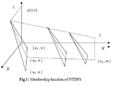
Let à be the fuzzy number whose components are the elements ofR × N, Rbeing the set of real numbers and N being the set of natural numbers with the membership grade satisfying the functional relationμ:R × N → 0,1 .Now asn → ∞ifμ(x,n) → 1for somex ∈ R and n ∈ N then we call the set à as dense fuzzy set. If à is triangular then it is called TDFS. Now, if for someninN,μ(x,n)attains the highest membership degree 1 then the set itself is called “Normalized Triangular Dense Fuzzy Set” or NTDFS.
Example 1 As per definitions (1) let us assume the NTDFS as follows
1 t1th , , 1 t1th , for 0 , 1, h 0 and the membership function along with graphical illustration ( Fig.-1) is given by
,h
0 t 1 t1th h‹ 㐱 (1 t1th)
t 1t1th
1th t (1 t1th) 1t1tht
1th t (1 t1th)
Definition 2: [ De[18]] Let the TDFSA a 1 t ρf
n ,a,a 1 t σgn for0 ρ, σ ∈ Rand
fn,gnare two Cauchysequences of functions having converging points respk11 and k1, 0 ≠ k1, k ∈ Rectively, then the
fuzzy set Ais called triangular dense fuzzy lock set with double keys k1and k , and they depend upon ρ and σ,
respectively. The corresponding membership function of Ais stated in (2), and its graphical representation is given by Fig. 2.
,h
0
t
1 t t
hh‹ 㐱 1 t
ht 1t th
th
t 1 t t
h1t h t
h
t
1 t
h(2)
( ,h)
Fuzzy Lock
1 N
1,h ,h ,h
,h
X 1
Fig 2: Membership function of TDFLS
We assume, fn k11tnt11 and gn k1 tnt11 in the above fuzzy set ( 2) and we have the left and the right
α-cuts of a triangular dense fuzzy number A μ(x,n) as follows:
μLd, μ R
d a t aρ α t 1 1 k1t
1
nt1 , a t aσ 1 t α 1 k t
1 nt1
The corresponding index value is given by
I x 1N n 1N 01 μLdt μ R
d dα a ta 4
σ k t
ρ k1 t
a ρtσ 4N
1t1t … t 1
Nt1 (3)
[ for details see (16)]
3. Assumptions and Notations
Notations
C1:Holding cost per quantity per unit time($) C :Shortage cost per unit quantity per unit time($)
C :Set up cost per unit time period per cycle ($)
D :Demand in shortage period D D1ett Q1:Inventory level within timet1(days) Q :Shortage quantity during the time t (days) t1:Inventory run time (days)
t :Shortage time(days) T: Cycle time ( t1 t t )(days)
TAC: Total average cost ($)
Assumptions
We have the following assumptions 1. Demand rate is uniform and known 2. Rate of replenishment is finite 3. Lead time is zero/negligible
4. Shortage are allowed and fully backlogged
4. Formulation of Crisp Mathematical Model
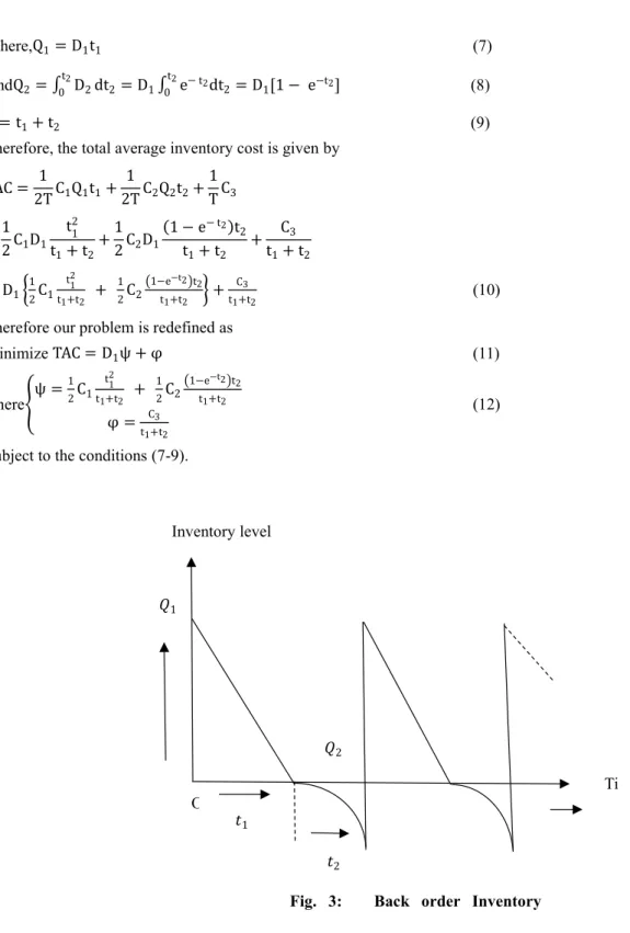
Let the inventory starts at time t = 0 with order quantity Q1 and demand rateD. After time t t1 the inventory reaches
zero level and the shortage starts and it continues up to timeT t1 t t ). Let Q be the shortage quantity during that
time periodt . Also, we assume that the shortage time demand rate is depending on the duration of shortage time
t .Therefore, the mathematical problem associated to the proposed model is shown in Fig.-4 and the necessary calculations are given below.
Inventory holding cost 1C1Q1t1 (4)
Shortage cost 1C Q t 1C D1 1 t et t t (5)
Where,Q1 D1t1 (7)
AndQ 0t D dt D1 0t et tdt D
1[1 t ett ] (8)
T t1t t (9)
Therefore, the total average inventory cost is given by
TAC 1TC1Q1t1t 1TC Q t t1TC 1
C1D1t t1 1t t t
1
C D1 1 t e t t t t1t t t
C t1t t
= D1 1C1t1ttt1 t 1C 1te tt t t1tt t
C
t1tt (10)
Therefore our problem is redefined as
MinimizeTAC D1ψ t φ (11)
where ψ
1C
1t1ttt1 t 1C 1te tt t t1tt φ tC
1tt
(12) Subject to the conditions (7-9).
Inventory level
1
O
1
T meTi
Fig. 3: Back order Inventory model
5. Fuzzy Mathematical Model
Since demand rate follows an important role in defining the objective function in an inventory process, so we consider the demand rate assumes flexible values in the propose model and it can be reduce by means of dense fuzzy set. So the objective function( TAC Z)of the crisp model (11) can be written as
Whereψandφare given by (12). Now, (11) can also be written as
D1 (Ztφ)ψ and its fuzzy equivalent is given by D1 (Z tφ)ψ (14)
Now, if we think of the demand rate assumes triangular dense fuzzy lock set then as per De[18]the membership function
of the demand rate is given by
μ D1
dtd0 1tρ k11tnt11
d0ρ k11tnt11 , if d0 1 t ρ 1 k1t
1
nt1 d d0 d0 1tσ k1tnt11 td
d0σ k1tnt11 , if d0 d d0 1 t σ 1 k t
1 nt1 0, if d d0 1 t ρ k11tnt11 and d d0 1 t σ k1 tnt11
(15)
The left and right α tcuts of the μ D1 are μLd, μRd d0t d0ρ α t 1 k11tnt11 , d0t d0σ 1 t α k1 tnt11
The corresponding index value is given by
I D1 1N n 1N 0 1
μLdt μ R d dα 1
N n 1 N
0 1
d0t d0ρ α t 1 k11tnt11 t d0σ 1 t α k1 tnt11 dα 1
N n 1
N d
0td0ρ 1k1tnt11 td0σ 1k tnt11 1
N n 1N d0t d0 σ
k t ρ k1 t
d0
nt1 ρ t σ
d0td40 kσ tkρ1 td04Nρtσ 1t1t … tNt11 (16)
Now we obtain the membership function of the fuzzy objective by using (14) in (15)
μ Z
Ztφ
ψ td0 1tρ k11tnt11
d0ρ k11tnt11 , if d0ψ 1 t ρ 1 k1t
1
nt1 t φ Z d0ψ t φ d0 1tσ k1tnt11 tZtφψ
d0σ k1tnt11 , if d0ψ t φ Z d0ψ 1 t σ 1 k t
1 nt1 t φ
0 , elsewhere
(17)
Now the left and rightα tcuts ofμ Z are given by
μLZ, μ R
Z φ t d
0ψ t d0ψρ k11tnt11 α t 1 ,φ t d0ψ t d0ψσ k1tnt11 1 t α
The corresponding index value is
I Z 1N n 1N 0
1 μLZt μ
R
Z dα 1
N n 1N 0 1
φ t d0ψ t d0ψρ k11tnt11 α t 1 t d0ψσ k1 tnt11 1 t
α dα 1N n 1N φ t d0ψ td0ψρ 1k1tnt11 td0ψσ 1k tnt11 φ t d0ψ td04ψ kρ1tkσ td0ψ ρtσ4N 1t1t … t 1
5.1 Particular Cases
1. If we take k1 k kthen
2. I Z φ t d0ψ td0ψ ρtσ4k td0ψ ρtσ4N 1t1t … tNt11
I D1 d0td04kσtρ td04Nρtσ 1t1t … tNt11 (19)
gives the problem of dense fuzzy lock model for single key. 3. If we take k1 k 1then
4. I Z φ t d0ψ td0ψ ρtσ4 td0ψ ρtσ4N 1t1t … tNt11
I D1 d0td0σtρ4 td04Nρtσ 1t1t … tNt11 (20)
gives the problem of dense fuzzy model. 5. If we take k1 k 1andN→ ∞then
I Z φt d0ψ−d0ψ ρ−σ
4 and I D1 d0t d0σ−ρ
4 (21)
gives the problem of general fuzzy model.
6. If we take k1 k 1andN→ ∞and ρ σ then
I Z φt d0ψ and I D1 d0 (22)
Gives the problem of crisp model.
5.2 [De
[18]]Rules of Finding Key Values of the Fuzzy Locks
When an uncertainty appears in a parameter, then the expert may not know the exact value but (s)he knows a bound of that parameter. Then (s)he usually fixes a upper limit (aU, if known), lower limit (aL, if known) or both for that
parameter.For single key, if upper bound is available then the index value of a is given byI a aUimplies a σtρ 4 aUta .
If the lower bound is known, thenI a aLimplies a ρtσ
4 ataL . For double keys the index value ofA is given by I A 1N n 0N
0 1
Lt1 α,n t Rt1 α,n dα a 1 t ρ k1 t
a 1 t σ k ,
So, a 1 t ρk 1 a
L⇒ k
1 at aaρ L and a 1 t kσ aU⇒ k aaσUta .
6. Numerical Example 1
Let us consider C1 .5, C 1.8, C 1 00, d1 100, ρ 0. , σ 0. then we get the following results.Here we
keep the bounds of demand rate stated as under d0L,d 0
U 90, 110 . Employing the above definition of finding the
keys we write,
k1 k
d0ρ d0t d0L
d0σ d0Ut d
0
100 × 0. 100 t × 90
100 × 0. × 110 t 100
t 0.187 0.08
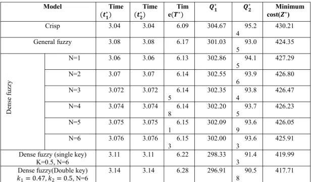
Table 1:Optimal solution of EOQ model
Model Time
(‴ ) (‴ )Time e( )Tim cost( )Minimum
Crisp 3.04 3.04 6.09 304.67 95.2
4 430.21
General fuzzy 3.08 3.08 6.17 301.03 93.0
5 424.35 D en se fu zz y
N=1 3.06 3.06 6.13 302.86 94.1
5 427.29
N=2 3.07 3.07 6.14 302.55 93.9
6 426.80
N=3 3.072 3.072 6.14
5 302.35 4 93.8 426.47
N=4 3.074 3.074 6.14
8 302.20 5 93.7 426.23
N=5 3.075 3.075 6.15
1 302.09 9 93.6 426.05
N=6 3.076 3.076 6.15
3 302.00 3 93.6 425.91
Dense fuzzy (single key)
K=0.5, N=6 3.11 3.11 6.22 298.33 3 91.4 419.99
Dense fuzzy(Double key) 1 0.47, 0.5, N=6
3.14 3.14 6.28 296.91 90.5
8 417.71
From the above Table1 we see that, the minimum objective value came from the dense fuzzy (double key) model having average inventory cost $ 417.71 for 6.28 days cycle time with 296.91 units of order quantity with respect to the 90.58 units of backorder quantity. The objective values for the other cases are of ascending order. It is also seen that, within 6 days week if we consider the learning experiences with at most 6 times interactions among retailer –supplier then the optimality comes for all the cases of dense fuzzy environment.
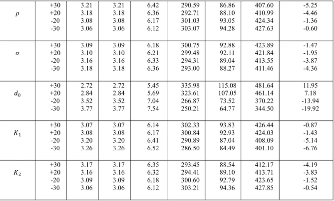
6.1 Sensitivity Analysis
Based on the numerical example (Case of dense fuzzy lock sets with double key) considered above for the single production plant model, we now calculate the corresponding outputs for changing inputs parameter one by one. The sensitivity analysis is performed ( See Table-2) by changing of each parameterC1, C , C , ρ, σ, k1,k and d0by +30%,
+20%, -20% and -30% considering one at a time and keeping the remaining parameters as unchanged. Table 2:Sensitivity analysis with parametric changes from (-30% to +30%) Para
meter Change% ‴days ‴days days Minimum
cost (t) t tt 1 +30 +20 -20 -30 2.74 2.86 3.51 3.76 2.74 2.86 3.51 3.76 5.48 5.71 7.02 7.52 259.86 270.63 332.68 356.15 88.61 89.26 91.88 92.50 469.68 453.11 378.49 356.99 9.17 5.32 -12.02 -17.01 +30 +20 -20 -30 3.11 3.12 3.14 3.15 3.11 3.12 3.14 3.15 6.23 6.25 6.29 6.30 295.48 295.96 297.85 298.32 90.52 90.54 90.62 90.64 429.94 425.86 409.56 405.48 -0.06 -1.01 -4.79 -5.74 +30 +20 -20 -30 3.59 3.45 2.78 2.59 3.59 3.45 2.78 2.59 7.18 6.90 5.57 5.18 340.44 326.58 263.90 245.75 92.10 91.69 88.86 87.63 471.20 454.17 377.18 354.88 9.52 5.57 -12.32 -17.51
+30 +20 -20 -30 3.21 3.18 3.08 3.06 3.21 3.18 3.08 3.06 6.42 6.36 6.17 6.12 290.59 292.71 301.03 303.07 86.86 88.10 93.05 94.28 407.60 410.99 424.34 427.63 -5.25 -4.46 -1.36 -0.60 +30 +20 -20 -30 3.09 3.10 3.16 3.18 3.09 3.10 3.16 3.18 6.18 6.21 6.33 6.36 300.75 299.48 294.31 293.00 92.88 92.11 89.04 88.27 423.89 421.84 413.55 411.46 -1.47 -1.95 -3.87 -4.36 ‹0 +30 +20 -20 -30 2.72 2.84 3.52 3.77 2.72 2.84 3.52 3.77 5.45 5.69 7.04 7.54 335.98 323.61 266.87 250.21 115.08 107.05 73.52 64.77 481.64 461.14 370.22 344.50 11.95 7.18 -13.94 -19.92 1 +30 +20 -20 -30 3.07 3.08 3.20 3.26 3.07 3.08 3.20 3.26 6.14 6.17 6.41 6.52 302.33 300.84 290.89 286.50 93.83 92.93 87.04 84.49 426.44 424.03 408.09 401.10 -0.87 -1.43 -5.14 -6.76 +30 +20 -20 -30 3.17 3.16 3.09 3.06 3.17 3.16 3.09 3.06 6.35 6.32 6.18 6.12 293.45 294.41 300.60 303.21 88.54 89.10 92.79 94.36 412.17 413.71 423.65 427.85 -4.19 -3.83 -1.52 -0.54
6.2 Discussion on Sensitivity Analysis
Table 2 shows that the shortage cost per unit item C , the fuzzy system parametersρ ,σ and the decision makers’ choices K1 and K are slightly sensitive towards model minimum ( unidirectional ) with reference to all the changes
from -30% to +30 %. For these parameters the objective values (average inventory cost) getting range from $ 405.48 to $ 429. 94 for the range of the order quantity 290.59- 303 only. 21 units with maximum cycle time duration 6.52 days only. We also notice that, the order quantity, the backorder quantity and the average cost functions have simple proportional changes. But for the other parameters, all the changes assume similar directional average (considerable) changes. Throughout the whole table we see if we reduce the demand parameter -30% then the average inventory cost reaches value to $ 344.50. Moreover, if we consider the case of single key then for its -30% change can give the model minimum $ 401.10 alone. However, if the system itself has double decision maker over single decision, then keeping the first one’s perception value fixed and increasing the second other’s to +30 % we can arrive at the average inventory cost value to $ 412.17 exclusively.
6.3 Graphical Illustrations of the Model
We have studied graphically over the numerical outputs ( Table- 1) of the model. The Fig.-4 shows the average cost values of the model began to decrease whenever we are going through Crisp environment to dense fuzzy lock rule of double keys. We may note that, the key value of decision maker one corresponds to the choice of perception over the system and that for the other corresponds to the second decision maker also. Although, Fig-5 reveals that, over the changes of the fuzzy system parameters ( , σ ) the average inventory cost axis revolves around the fuzzy system parameters itself. The unit holding cost, the set up cost and the demand parameters ate most fluctuating parameters getting objective values around 344-481. The variations of the cost functions are negligible for the fuzzy system parameters and the keys also.
7. Conclusion
Here we have discussed a simple backorder EOQ model under double decision maker for single decision under dense fuzzy environment. The novelty of this article is that it expresses the shortage time demand as exponentially decaying with the duration of the shortage time. However, the present article deserve that the concept of single decision maker in a inventory process is vague with certain extent rather it would be beneficial if we consider the multiple decision maker within democratic attitude by means of healthy inter relationship among the hierarchy of the management process over strategic understanding.
References
1. Baez-Sancheza A D, Morettib A C, Rojas-Medarc M A, 2012, On Polygonal Fuzzy Sets and Numbers. Fuzzy Sets and System,
209: 54–65.
2. Ban A I, Coroianu L, 2014, Existence, Uniqueness and Continuity of Trapezoidal Approximations of Fuzzy Numbers Under a
General Condition. Fuzzy Sets and System, 257: 3–22.
3. Beg I, Ashraf S, 2014, Fuzzy Relational Calculus. Bulletin of the Malaysian Mathematical Science Society, 37(1): 203–237.
4. Bellman E, Zadeh L A, 1970, Decision Making in a Fuzzy Environment. Management Sciences, 17(4): 141–164.
5. Chutia R, Mahanta S, Baruah H K, 2010, An Alternative Method of Finding the Membership of a Fuzzy Number. International
6. Das P, De S K, Sana S S, 2014, An EOQ Model for Time Dependent Backlogging Over Idle Time : A Step Order Fuzzy Approach. International Journal of Applied and Computational Mathematics, 1(2): 1–17.
7. Deli I, Broumi S, 2015, Neutrosophic Soft Matrices and NSM-decision making. Journal of Intelligent and Fuzzy System, 28(5): 2233–2241.
8. De S K, Beg I, 2016, Triangular Dense Fuzzy Sets and New Defuzzication Methods. Journal of Intelligent and Fuzzy System, 31(1): 467–479.
9. De S K, Beg I, 2016, Triangular Dense Fuzzy Neutrosophic Sets. Neutrosophic Sets and Systems, 13: 1–12.
10. De S K, 2013, EOQ Model with Natural Idle Time and Wrongly Measured Demand Rate. International Journal of Inventory Control and Management, 3(1–2): 329–354.
11. De S K, Goswami A, Sana S S, 2014, An Interpolating by Pass to Pareto Optimality in Intuitionistic Fuzzy Technique for an EOQ Model with Time Sensitive Backlogging. Applied Mathematics and Computation, 230: 664–674.
12. De S K, Mahata G C, 2016, Decision of a Fuzzy Inventory with Fuzzy Backorder Model Under Cloudy Fuzzy Demand Rate, International Journal of Applied and Computational Mathematics.
13. De S K, Sana S S, 2015,An EOQ Model with Backlogging. International Journal of Management Sciences and Engineering Management.
14. De S K, Sana S S, 2013, Backlogging EOQ Model for Promotional Effort and Selling Price Sensitive Demand an Intuitionistic Fuzzy Approach. Annals of Operations Research.
15. De S K, Sana S S, 2013, Fuzzy Order Quantity Inventory Model with Fuzzy Shortage Quantity and Fuzzy Promotional Index. Economic Modelling, 31: 351–358.
16. De S K, and Sana S S, 2014, An Alternative Fuzzy EOQ Model with Backlogging for Selling Price and Promotional Effort Sensitive Demand. Int J of Applied and Computational Mathematics, 1–20.
17. De S K, Sana S S, 2016, The (p, q, r, l) Model for Stochastic Demand Under Intuitionistic Fuzzy Aggregation with Bonferroni Mean. Journal of Intelligent Manufacturing, 1–21.
18. De S K, 2017, Triangular Dense Fuzzy Lock Set. Soft Computing.
19. Diamond P, Kloeden P E, 1991, Parametrization of Fuzzy Sets by Single Valued Mappings, Proc 4th IFSA, Brussels, 42–45. 20. Diamond P, 1989, The Structure of Type Fuzzy Numbers, in the Coming of Age of Fuzzy Logic J C Bezdek (ed.), Seattle,
671–674.
21. Diamond P, 1990, A Note on Fuzzy Star Shaped Fuzzy Sets. Fuzzy Sets and Systems.
22. Diamond P, Kloeden P E, 1989, Characterization of Compact Sets of Fuzzy Sets. Fuzzy Sets and Systems. 29: 341–348. 23. Dubois D, Prade H, 1978, Operations on Fuzzy Numbers. International Journal of System Science. 9(6): 613–626. 24. Goetschel R, Voxman J, 1985, Eigen Fuzzy Number Sets. Fuzzy Sets and System, 16(1): 75–85.
25. Heilpern S, 1981, Fuzzy Mappings and Fixed Point Theorem. J Math Anal Applns, 83: 566–569.
26. Kaufmann A, Gupta M M, 1985, Introduction of Fuzzy Arithmetic Theory and Applications. Van Nostrand Reinhold, New York.
27. Kazemi N, Ehsani E, Jaber M, 2010, An Inventory Models with Back Orders with Fuzzy Parameters and Decision Variables. International Journal of Approximate Reasoning, 51(8): 964–972.
28. Kazemi N, Olugu E U, Salwa Hanim A R, Ghazilla R A B R, 2015, Development of a Fuzzy Economic Order Quantity Model for Imperfect Quality Items Using the Learning Effect on Fuzzy parameters. Journal of Intelligent and Fuzzy System, 28(5):2377–2389.
29. Kazemi N, Olugu E U, SalwaHanim A R, Ghazilla R A B R, 2016, A Fuzzy EOQ Model with Backorders and Forgetting Effect on Fuzzy Parameters: An Empericalstudy. Computers and industrial Engineering, 96: 140–148.
30. Kazemi N, Shekarian E, Cárdenas-Barrón L E , Olugu E U, 2015, Incorporating Human Learning into a Fuzzy EOQ Inventory Model with Backorders. Computer and Industrial Engineering, 87: 540–542.
31. Mahanta S, Chutia R, Baruah H K, 2010, Fuzzy Arithmetic Without Using the Method of α –Cuts. International Journal of
Latest Trends in Computing, 73–80.
32. Piegat A, 2005, A New Definition of Fuzzy Set. Appl Math Comput Sci, 15(1):125–140.
33. Roychoudhury S, Pedrycz W, 2003, An Alternative Characterization of Fuzzy Complement Functional. Soft Computing – A Fusion of Foundations, Methodologies and Applications, 563565.