A multi-objective mathematical model for production-distribution
scheduling problem
Farshad Aghajani
1, S. Mohammad J. Mirzapour Al-e-Hashem
1*1Department of Industrial Engineering and Management Systems, Amirkabir University of Technology (Tehran Polytechnic), Iran
[email protected], [email protected]
Abstract
With increasing competition in the business world and the emergence and development of new technologies, many companies have turned to integrated production and distribution for timely production and delivery at the lowest cost of production and distribution and with the least delay in delivery. By increasing human population and the increase in greenhouse gas emissions and industrial waste, in recent years the pressures of global environmental organizations have prompted private and public organizations to take action to reduce environmental pollutants. This paper presents a nonlinear mixed integer model for the production and distribution of goods with specified shipping capacity and specific delivery time for customers. The proposed model is applicable to flexible production systems; it also provides routing for the means of transportation of products, as well as the reduction of emissions from production and distribution. The model is presented, and then by mathematical linearization is transformed into a mixed integer linear model. The data of a furniture company is used to solve the linear model, and then the linear model with the company data is solved by CPLEX software. The numerical results show that as costs increase, delays are reduced and consequently, customer satisfaction increases, and as costs increase the air pollution decreases.
Keywords: Production-distribution integration, production scheduling, routing, job shop, green supply chain, timely delivery
1-Introduction
The first step to managing is planning. Planning means to select measurable goals and making decisions to achieve these goals. Planning is a prerequisite for execution and control and without these two, it cannot be completed. At the core of supply chain management issues are production and distribution planning. The issue of production planning in the supply chain is the decisions made by the manufacturer to produce the ordered product and its timing and number in order to fulfil the customer's need. The issue of distribution planning in the supply chain also includes decisions to find a way to deliver goods from a manufacturer to a distributor or to a customer. These issues are interrelated, so they must be applied simultaneously in an integrated way to reduce (increase) the costs (benefits) resulting from them.
*Corresponding author
ISSN: 1735-8272, Copyright c 2020 JISE. All rights reserved
Journal of Industrial and Systems Engineering
Vol. 13, Special issue: 16th International Industrial Engineering Conference Winter (January) 2020, pp. 121-132
(IIEC 2020)
TEHRAN, IRAN
22-23 January 2020
122
Based on past research, the integrated models presented in the supply chain can be categorized as follows:
• Buyer-seller integrated models
• Integrated Production - Distribution Planning Models • Integrated production - inventory planning models • Location-allocation models
One of the most important issues in the supply chain is integrated production-distribution planning. The integrated production and distribution of products in a supply chain plays an important role in minimizing chain costs. In order to achieve optimal performance in the supply chain, it seems necessary to integrate the two parts of production and distribution. The use of integrated production and distribution scheduling has more advantages than the use of decentralized and coordinated production and distribution schedules. For this reason, the topic of integrated production and distribution scheduling is one of the most important issues that have recently received much research in the field of production management and supply chain.
Investing in improving the environmental performance of the supply chain has many benefits, including saving energy resources, reducing pollutants, eliminating or reducing waste, creating value for customers, and ultimately enhancing productivity for companies and organizations. Producers went beyond what was needed in the late 1980s and moved to a greener approach to system operation. Green Supply Chain Management seeks not to produce or reduce waste (energy, greenhouse gas, chemical / hazardous waste, solid waste) throughout the supply chain. Environmental issues under the law and consumer guidelines, particularly in the United States, the European Union and Japan, have become a major concern for manufacturers. As a critical innovation, it helps organizations develop green supply chain management strategies to achieve shared profit and market goals by reducing environmental risks and enhancing their environmental productivity.
2-Literature review
Li et al. (2016) considered a set of multi-objective distribution-production scheduling issues with a production machine and several carriers. The goal is to minimize shipping cost and overall customer waiting time. Gharaei and Jolai (2018), studied on supply chain integration. One of the most interesting is integrating production scheduling and distribution decisions.
Mirzapour Al Hashem et al. (2011) stated that the manufacturers must meet customer demands in order to compete in the real world. This requires optimal performance and efficient supply chain design. In this research, they have investigated a supply chain involving multiple suppliers, multiple manufacturers, and multiple customers by addressing the issue of multi-product mass production, multi-cycle and multi-product planning under uncertainty. Mirzapour Al Hashem et al. (2013) developed a stochastic programming approach to solve a period, product, and multi-location mass production design problem in a green supply chain for a medium design period under the assumption of demand uncertainty.
Boutarfa et al. (2016) studied an integrated design and production planning - distribution problem within a specific supply chain structure. This model involves a supplier that produces a single product and supplies it to its customers. Sreeram et al. (2015) addressed a multi-objective production-distribution problem to minimize the cost of overall arrival delay and overall production-distribution cost. This is an NP-Hard problem with two goals. The first is to sort orders on a production line in such a way as to reduce this order delay, and the second is to transfer orders by considering a heterogeneous fleet of vehicles and thereby reducing distribution costs.
Senousi et al. (2018) considered integrating production, inventory and distribution decisions into a supply chain including a single supplier and several retailers. Gao et al. (2015) studied a type of integrated production and distribution problem in which orders are processed and delivered in batches or groups with limited vehicle capacity. This emphasizes the unexpected conditions between production and distribution of each batch. Devapriya et al. (2017) focuses on the problem of a perishable product that must be produced and distributed at the lowest cost before it perishes.
Rafiei et al., (2018) Integrated Production Planning - Distribution that reduces costs, increases supply chain efficiency. Fan et al. (2015) studied the problem of integrated production and distribution scheduling on a single machine. Due to the machine’s limited availability, its activities
123 and tasks may be terminated at its operation period.
Wang and Wang (2013) stated that the job shop production scheduling issue is an NP-Hard problem. An inventory-based two-objective Job shop production scheduling model is presented in their research in which both the make span (total completion time) and inventory holding cost have been optimized simultaneously. Darwish and Coelho (2018) have introduced a production-distribution system that addressed the location, production, inventory and distribution decisions, simultaneously. The goal is to minimize overall costs during estimating demand at delivery time.
Mohammadi et al. (2020) developed a bi-objective mixed integer problem, in which the first objective function aims to minimize a sum of the production and distribution scheduling costs, and the second objective function tries to minimize a weighted sum of delivery earliness and tardiness, they ignored to consider the environmental factors of the production and distribution.
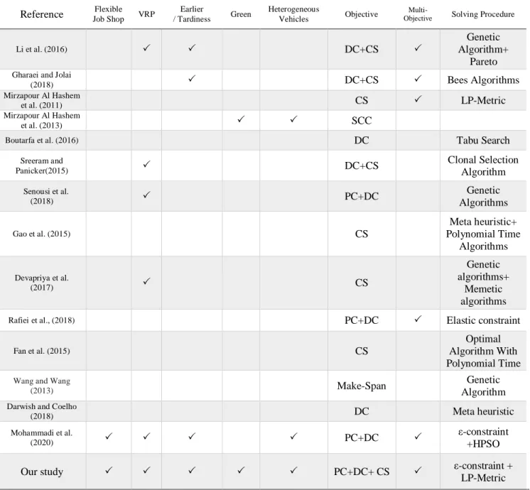
Table 1. Overview of the related integrated production-distribution scheduling (IPDS) studies Reference Job Shop Flexible VRP Earlier
/ Tardiness Green
Heterogeneous
Vehicles Objective
Multi-Objective Solving Procedure
Li et al. (2016) DC+CS
Genetic Algorithm+
Pareto
Gharaei and Jolai
(2018) DC+CS Bees Algorithms
Mirzapour Al Hashem
et al. (2011) CS LP-Metric
Mirzapour Al Hashem
et al. (2013) SCC
Boutarfa et al. (2016) DC Tabu Search
Sreeram and
Panicker(2015) DC+CS
Clonal Selection Algorithm
Senousi et al.
(2018) PC+DC
Genetic Algorithms
Gao et al. (2015)
CS
Meta heuristic+ Polynomial Time
Algorithms
Devapriya et al.
(2017) CS
Genetic algorithms+
Memetic algorithms
Rafiei et al., (2018) PC+DC Elastic constraint
Fan et al. (2015) CS
Optimal Algorithm With Polynomial Time
Wang and Wang
(2013) Make-Span
Genetic Algorithm
Darwish and Coelho
(2018) DC Meta heuristic
Mohammadi et al.
(2020) PC+DC
ε-constraint +HPSO
Our study PC+DC+ CS ε-constraint +
LP-Metric SCC: Supply Chain Cost; CS: Customer satisfaction; DC: Distribution cost; PC: Production cost
124
3- Problem Definition
Production takes place in a flexible job shop production system with a set of available multi-purpose machines. Each section contains a specific set of processes; each of them can be processed by different types of machines at different processing times and costs. However, each process must be processed by one of the relevant machines, while each machine and device can process only one process at a time. Therefore, the production department must determine which process should be assigned to each machine through a specific set and how the assigned process can be scheduled. On the other hand, transportation is done with a limited number of vehicles with different capacities and fixed costs. Once the products have been completed, they are grouped together for delivery to the customers so that each category is delivered with one of the vehicles delivered to the respective customer. In addition, the overall size of each category of delivery shall not exceed the capacity of the vehicle. Each vehicle is initially deployed at the production site and returned to the production site after service on the specified route. In addition, it is assumed that the start time of each batch is equal to the time of completion of the last order of that batch. The distribution department should therefore determine how much cargo each vehicle can carry, which customer will be served on the journey, how the order is delivered on each journey, and when each cargo departs from the manufacturing site, and the correct allocation manufactured machinery in terms of the amount of waste produced for each product, as well as the allocation of vehicles from the point of view of the amount of carbon dioxide produced by the routes. The problem is modelled as a production and distribution scheduling framework and a multi-objective complex integer model trying to identify the best route and schedule of operations from the machines, optimally arrange the vehicles, routes and the ideal time of moving the vehicles from the production site. In order to meet three contradictory objectives simultaneously, we propose to minimize production and distribution scheduling costs and minimize the total weight of delay and early delivery and to reduce the emissions from production and distribution. In the proposed model the distribution cost includes a fixed cost for each vehicle used and a variable cost for the total distance travelled by the vehicles. In addition, it should be noted that since in a job shop production environment an order can be processed by a variety of machines and devices available, it is important to consider production costs as an important overall cost component to minimize scheduling costs at the manufacturing site. In addition, due to the flexible machine environment in which each operation can be processed by a variety of machines and devices and by different processing times, the cost of producing a function of machine configuration and operation is designed. The pollutants include waste from the production of each car and the amount of carbon dioxide gas in each vehicle.
4-Modeling
4-1-Model assumptions
The following assumptions have been used to solve the model. • The capacity of the vehicle is known.
• The delivery time for customers is already known. • Time window is considered.
• Different means of transport are considered. • Workshop flexible production system
• Each process is handled by one or more machines. • Disconnection is not allowed.
• Operation time is constant.
4-2-Symbols
In this section, the symbols used throughout the problem are presented as follows:
Collections:
The set of sections, shown by 𝑖, 𝑗 𝜔 = {1, … , 𝑁}
The set of operations of section j, represented by 𝑓, 𝑟 𝜂𝑗 = {1,2, … , 𝑅𝑗}
A set of devices, denoted by 𝑚 𝛷 = {1,2, … , 𝑀}
125
The set of available vehicles, shown by 𝑣 𝛺 = {1,2, … , 𝑉}
Parameters:
Cost of unit production per unit time
𝜆𝑚
Fixed cost of vehicle
𝐹𝑣
Variable cost of vehicle per unit of time
𝜃𝑣
Early delivery weight
𝜇
Delayed delivery weight
𝜑
Order processing time on device
𝑃𝑗𝑟𝑚
Process Matrix - A machine that has a value of 1 if it provides a machine or machine with the ability to process operations from a segment otherwise it is equal to 0
𝑎𝑗𝑟𝑚
Shipping time from customer to customer j by vehicle
𝑡𝑖𝑗𝑣
Order size
𝛿𝑗
Order Delivery Time Range
(𝑎𝑗. 𝑏𝑗)
Vehicle capacity
𝑄𝑣
Weight of production waste (specific pollution factor of transport weight)
𝛾
If the process is done from scratch to the machine, the size of the waste (which means waste to the machine) is created. (The product of both the percentage of waste and the weight of the parts)
𝑊𝑗𝑟𝑚
The amount of greenhouse gas (GHG) produced per unit of time by the engine and vehicle.
𝑔𝑣
Decision variables:
Producing section
r Production start time of order operation
𝜋𝑗𝑟
Time to complete r order operations
𝛶𝑗𝑟
Order completion time
𝐶𝑗
A binary variable that has a value of 1 if the order processing is processed by the device, otherwise it is 0.
𝑋𝑗𝑟𝑚
A binary variable that takes a value of 1 if the order operation is processed immediately after executing the order on the machine, otherwise it is 0.
𝑌𝑖𝑓𝑗𝑟𝑚
Distribution section
Order Delivery Time
𝐷𝑗
Time of customer visit by vehicle
𝑇𝑗𝑣
Time to leave the vehicle from the place of production
𝑆𝑣
Time to visit the last customer on the vehicle route
𝐸𝑣
A binary variable that takes a value of 1 if the order is delivered by the vehicle, otherwise it is 0.
𝑍𝑗𝑣
A binary variable that takes the value 1 if the order is delivered after order 𝑖 and otherwise is 0.
𝑈𝑖𝑗𝑣
A binary variable that takes a value of 1 if the vehicle is used for delivery otherwise it is 0.
126
4-3- Mathematical model
The integrated production-distribution scheduling problem has been checked and is formulated as the following nonlinear mixed integer model:
𝑚𝑖𝑛 𝑓1= ∑ ∑ ∑ 𝜆𝑚𝑃𝑗𝑟𝑚𝑋𝑗𝑟𝑚
𝑀 𝑚=1 𝑅𝑗 𝑟=1 𝑁 𝑗=1 ⏟ 𝑓11
+ ∑[𝐹𝑣𝑊𝑣+𝜃𝑣(𝐸𝑣− 𝑆𝑣)]
𝑉
𝑣=1
⏟
𝑓12
(1)
𝑚𝑖𝑛 𝑓2 = 𝜑 × ∑ 𝑚𝑎𝑥(𝐷𝑗− 𝑏𝑗. 0)
𝑁
𝑗=1
+ 𝜇 × ∑ 𝑚𝑎𝑥(𝑎𝑗− 𝐷𝑗. 0)
𝑁
𝑗=1
(2)
𝑚𝑖𝑛 𝑓3= 𝛾 × ∑ ∑ ∑ 𝑊𝑗𝑟𝑚× 𝑋𝑗𝑟𝑚
𝑀 𝑚=1 𝑅𝑗 𝑟=1 𝑛 𝑗=1
+ (1 − 𝛾) × ∑ ∑ ∑ 𝑔𝑣× 𝑡𝑖𝑗𝑣× 𝑈𝑖𝑗𝑣
𝑉 𝑣=1 𝑛 𝑗=1 𝑛 𝑖=0 (3) Subject to:
∑ 𝑋𝑗𝑟𝑚
𝑀
𝑚=1
= 1 ∀𝑗 ∈ 𝜔 , ∀𝑟 ∈ 𝜂𝑗 (4)
𝑋𝑗𝑟𝑚≤ 𝑎𝑗𝑟𝑚 ∀𝑗 ∈ 𝜔 , ∀𝑟 ∈ 𝜂𝑗 , ∀𝑚 ∈ 𝛷 (5)
𝑋𝑖𝑓𝑚 = ∑ ∑ 𝑌𝑖𝑓𝑗𝑟𝑚
𝑅𝑗
𝑟=1 𝑁+1
𝑗=1
∀𝑖 ∈ 𝜔 , ∀𝑓 ∈ 𝜂𝑗 , ∀𝑚 ∈ 𝛷 (6)
𝑋𝑗𝑟𝑚= ∑ ∑ 𝑌𝑖𝑓𝑗𝑟𝑚
𝑅𝑗
𝑓=1 𝑁
𝑖=0
∀𝑗 ∈ 𝜔 , ∀𝑟 ∈ 𝜂𝑗 , ∀𝑚 ∈ 𝛷 (7)
𝜋𝑗𝑟≥ 𝑚𝑎𝑥 {𝛶𝑗(𝑟−1). ∑ ∑ ∑ 𝛶𝑖𝑓× 𝑌𝑖𝑓𝑗𝑟𝑚
𝑀 𝑚=1 𝑅𝑗 𝑓=1 𝑁 𝑖=0
} ∀𝑗 ∈ 𝜔 , ∀𝑟 ∈ 𝜂𝑗 (8)
𝛶𝑗𝑟= 𝜋𝑗𝑟+ ∑ 𝑃𝑗𝑟𝑚× 𝑋𝑗𝑟𝑚
𝑀
𝑚=1
∀𝑗 ∈ 𝜔 , ∀𝑟 ∈ 𝜂𝑗 (9)
𝐶𝑗= 𝛶𝑗𝑅𝑗 ∀𝑗 ∈ 𝜔 (10)
∑ ∑ ∑ 𝑌[0]𝑓𝑗𝑟𝑚= 1
𝑅𝑗 𝑟=1 𝑅0 𝑓=1 𝑁 𝑗=1
∀𝑚 ∈ 𝛷 (11)
∑ ∑ ∑ 𝑌𝑖𝑓[𝑁+1]𝑟𝑚= 1
𝑅𝑁+1 𝑟=1 𝑅𝑖 𝑓=1 𝑛 𝑖=1
∀𝑚 ∈ 𝛷 (12)
∑ 𝑍𝑗𝑣= 1
𝑉
𝑣=1
127
𝑍𝑗𝑣= ∑ 𝑈𝑖𝑗𝑣
𝑁
𝑖=0
∀𝑗 ∈ 𝜔 , ∀𝑣 ∈ 𝛺 (14)
∑ 𝑈𝑖𝑗𝑣= ∑ 𝑈𝑗𝑖𝑣
𝑁+1
𝑖=1 𝑛
𝑖=0
≤ 1 ∀𝑗 ∈ 𝜔 , ∀𝑣 ∈ 𝛺 (15)
∑ 𝑈[0]𝑗𝑣= ∑ 𝑈𝑖[𝑁+1]𝑣 ≤ 1 𝑁
𝑖=1 𝑁
𝑗=1
∀𝑣 ∈ 𝛺 (16)
∑ 𝑍𝑗𝑣𝛿𝑗≤ 𝑄𝑣
𝑁
𝑗=1
∀𝑣 ∈ 𝛺 (17)
𝑇[0]𝑣= 𝑆𝑣 = 𝑚𝑎𝑥𝑗∈𝜔 𝑍𝑗𝑣𝐶𝑗 ∀𝑣 ∈ 𝛺 (18)
𝑇𝑗𝑣= ∑ 𝑈𝑖𝑗𝑣(𝑇𝑖𝑣+ 𝑡𝑖𝑗𝑣)
𝑁
𝑖=0
∀𝑗 ∈ 𝜔 , ∀𝑣 ∈ 𝛺 (19)
𝐷𝑗= ∑ 𝑍𝑗𝑣𝑇𝑗𝑣
𝑉
𝑣=1
∀𝑗 ∈ 𝜔 (20)
𝐸𝑣= 𝑆𝑣+ ∑ ∑ 𝑈𝑖𝑗𝑣𝑡𝑖𝑗𝑣
𝑛+1
𝑗=1 𝑛
𝑖=0
∀𝑣 ∈ 𝛺 (21)
𝑊𝑣= 𝑚𝑎𝑥
𝑗∈𝜔 𝑍𝑗𝑣 ∀𝑣 ∈ 𝛺 (22)
𝑋𝑗𝑟𝑚, 𝑌𝑖𝑓𝑗𝑟𝑚, 𝑍𝑗𝑣, 𝑈𝑖𝑗𝑣, 𝑊𝑣∈ {0,1} ∀𝑖, 𝑗 ∈ 𝜔 , ∀𝑓, 𝑟 ∈ 𝜂𝑗,∀𝑣 ∈ 𝛺 , ∀𝑚 ∈ 𝛷 (23)
𝜋𝑗𝑟, 𝛶𝑗𝑟, 𝐶𝑗, 𝐷𝑗, 𝑇𝑗𝑣, 𝑆𝑣, 𝐸𝑣≥ 0 ∀𝑗 ∈ 𝜔 , ∀𝑟 ∈ 𝜂𝑗 , ∀𝑣 ∈ 𝛺 (24)
Equation (1) is the first objective function and represents the total cost of the production-distribution system including the cost of producing the unit 𝑓11 and the distribution cost of 𝑓12 . The latter involves
a fixed cost function of a number of vehicles, plus a variable cost function of the total distance traveled by the vehicles. Equation (2) introduces customer satisfaction and aims to minimize the sum of the early and late delivery weights. Equation (3) introduces environmental pollution and aims to minimize the waste of production machinery and greenhouse gases produced by vehicles. Constraint (4) guarantees that each operation of each order should be assigned to only one machine. Constraint (5) indicates that each operation of each order must be assigned to a machine capable of processing it. Constraints (6) and (7) limit the operation such that each operation on each device has only one operation before it and only one operation or operation after it. 0 and 𝑛 + 1 orders Mock orders have 0 processing time. At the start of each machine process, the operation 𝑟 of order 0 must first be processed and the operation r of order n + 1 must be processed later.
In addition, the completion time as well as the start time of 𝑟 operations belong to the order 0 and 𝑛 + 1. 0 (𝛶[0]𝑟 = 0 . 𝜋[0]𝑟= 0 . 𝛶[𝑛+1]𝑟= 0 . 𝜋[𝑁+1]𝑟 = 0). Constraint (8) ensures that each
operation of each order can be started at least once the processor operation (𝛶𝑗[𝑟−1]) on each device is
completed and the device is not busy. Constraint (9) calculates the time taken to complete each operation equal to its start time plus its processing time on the device. Constraint (10) calculates the time to complete each order 𝑗. Constraint (11) ensures that only one prime operation is processed on each 𝑚 device. Constraint (12) ensures that only one operation is processed on each 𝑚 device.
128
Constraint (13) indicates that each order should only be assigned to one available vehicle. Limitation (14) limits each order to each route for having only one order before it. Constraint (15) specifies that any vehicle must leave the place immediately after the delivery of the orders entrusted to the relevant customers. Constraint (16) ensures that each vehicle starts its route from the production site and returns only once. Here in the distribution scheduling, two fictitious orders are used to illustrate the issue that in each delivery category, order 0 moves first from the company and order 𝑛 + 1 returns at the end of each route. Constraint (17) ensures that the capacity of each vehicle is not greater than the total order size. Constraint (18) specifies that the time of departure of each vehicle is equal to the maximum time to complete the production of all orders in each category. Constraint (19) specifies that the delivery time of order 𝑗 in vehicle 𝑣 is equal to the time of delivery of the previous order 𝑖 by this vehicle, and the distance between customers 𝑖 and 𝑗. Constraint (20) indicates the delivery time of each order in each journey. Constraint (21) indicates that each time of each route is equal to the starting time of the production site plus the total time of the routes traveled by each vehicle. Constraint (22) determines which vehicle is to be used for delivery. Finally, constraints (23) and (24) specify the types of variables.
4-4-Linearization
Linear programming, or in other words linear optimization, is a mathematical method for finding the maximum and minimum linear functions with their own constraints and constraints. Its main use is in management and economics, but it is also widely used in engineering, including industrial engineering.
The proposed model is a nonlinear mixed integer-programming model. Before solving the model, some theoretical techniques are used to linearize the model.
4-4-1-Linearization of maximum and minimum
As observed in equation (2) and constraints (8) and (18), the maximum operator is used which is a nonlinear explicit expression. The 𝑚𝑎𝑥(𝑚𝑖𝑛) operator is set to linear when the IBM ILOG CPLEX is used with the 𝑚𝑎𝑥𝑙(𝑚𝑖𝑛𝑙) function. Theoretically, we use it for easy linearization of the proposed model. Assuming we have a general nonlinear expression as 𝑚𝑎𝑥(𝑥1. 𝑥2. 𝑥3. … . 𝑥𝑛) , this can be
given to a linear equivalent structure by introducing a new positive variable and a set of binary variables 𝑧𝑖 and by Add the following restrictions.
(25)
𝑚𝑎𝑥(𝑥1. 𝑥2. 𝑥3. … . 𝑥𝑛) → 𝑦
(26)
∀𝑖 = 1, … , 𝑛 𝑦 ≥ 𝑥𝑖
(27)
∀𝑖 = 1, … , 𝑛 𝑦 ≤ 𝑥𝑖+ 𝑀 × 𝑧𝑖
(28)
∑ 𝑧𝑖 ≤ 𝑛 − 1 𝑛
𝑖=1
Above, 𝑀 is an arbitrary large number. Relation (26) states that 𝒚 must be greater than 𝑥𝑖 because 𝒚
is maximum 𝑥𝑖. The relations (27) and (28) guarantee that for at least one unit 𝒊, y must be less than
or equal to 𝑥𝑖to prevent 𝒚 from approaching infinity. It should be stated that when a target function is
minimized, relations (27) and (28) are necessary but necessary when the objective function is maximized or multi-objective model structure is required.
4-4-2-Linearization of the multiplication of a positive variable into a binary variable (zero and one)
The model has two expressions as 𝑍𝑗𝑣× 𝑇𝑗𝑣 and 𝛶𝑖𝑓× 𝑌𝑖𝑓𝑗𝑟𝑚 , respectively, with constraint (19) and
part of the relation (8), and these expressions are clearly nonlinear. Without losing the generality, suppose we have an expression 𝑥 × 𝑧 - where 𝑥 is a positive variable and 𝑧 is a binary variable. In addition, by introducing a new subsidiary or positive auxiliary variable 𝑦 and adding the following
129
constraints, this model can be transformed into a linear structure as follows:
(29)
𝑥 ∙ 𝑧 → 𝑦
(30)
𝑥 − (1 − 𝑧) × 𝑀 ≤ 𝑦 ≤ 𝑥
(31)
𝑦 ≤ 𝑀 × 𝑧
Again, M is a large arbitrary number.
5-Solution method
As shown in section 3-4, the problem of integrated production-distribution scheduling is formulated as a three-objective model. Most scheduling models usually involve a problem of simultaneous optimization of a number of goals that can be in conflict. The purpose of such problems (known as multi-objective optimization problems) is to optimize several contradictory criteria simultaneously. Unlike single-objective models that generate a single optimal solution, multi-objective models represent a set of optimal solutions called Pareto optimal sets or dominant solutions that overlay solutions. Others are dominant. In fact, Pareto solutions are solutions that cannot improve one goal without reducing at least one other goal.
Due to the nature of NP-hard, both the problem of flexible workshop production system scheduling, the problem of vehicle routing, as well as the problem of reducing waste production and greenhouse gas emissions from transport vehicles, the proposed model can be NP- be hard. In order to solve the proposed problem in small and real cases, different exact techniques of multi-objective decision-making methods can be used.
5-1-Limit method (Epsilon (ε) constraint)
The nature of three-objective integrated production-distribution scheduling model allows us to apply some of the techniques of multi-objective decision-making to solve it for small-scale real-life examples. Multi-objective decision-making techniques are categorized as deductive, innovative, and interactive. Under a deductive approach, a multi-objective optimization model is transformed into a single-objective model and the decision maker prioritizes the solution. In innovative approach, the decision maker selects the most appropriate solutions from a set of optimally generated solutions, and in the interactive approach, decision maker searches and the priorities affect the direction in which possible space is examined. The ε constraint method is one of the organized innovative techniques under which one of the objective functions is optimized at each stage, while others are added as model constraints with the upper bound ε:
(32)
𝑚𝑖𝑛 𝑓1
Subject to:
(33)
𝑓2≤ 𝜀2
…
(34)
𝑓𝑛 ≤ 𝜀𝑛
In order to solve a multi-objective optimization problem with the ε constraint method, the following steps are required:
1. One of the objective functions is chosen as the primary objective to be optimized, and the other objectives become model constraints, given the upper limit 𝜀 for each of them.
2. First, each target function is optimized separately and then the distance 𝐼𝑖 = (𝑓𝑖∗. 𝑓𝑖−)
between the optimal values and the bad values of the target function 𝑓𝑖 = (𝑖 = 2. … . 𝑛)
is divided to a predetermined specified number, the values 𝜀2. … . 𝜀𝑛 are then calculated. 3. The problem created in step 1 is solved many times with different values of ε𝑖 by
130
Based on this information, to obtain the model using Epsilon constraint method, the obtained values of objective functions are calculated as follows:
Table 2. The values of the objective functions obtained by the Epsilon constraint method
Best value Worst value
objective functions
41838442.892204 62462000
𝒇𝟏
0 34768.299580084
𝒇𝟐
359.181786216 2748.016528
𝒇𝟑
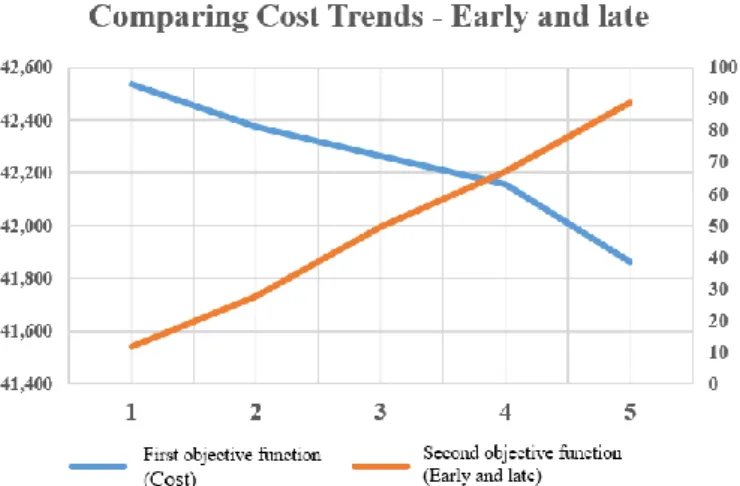
The behavior of the cost and early and late objective functions is shown in figure 1, which early and late functions decreases with the increase in the cost objective function.
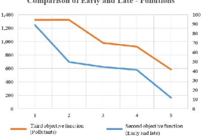
The behavior of the objective functions of the costs and pollution of production and transportation relative to each other is shown in figure 2, which with the increase in costs, air pollution and production waste decreases.
Fig 1. Comparison of the trend of cost-function and early and late objective functions
Fig 2. Comparison of objective functions of costs and pollution of production and transportation
131
As can be seen in figure 3, by comparing the target functions of the early and late and the production pollutants and transportation, we conclude that in order to reduce the early and delayed product delivery, the product segment must be delivered on time to the distribution part to be delivered on time.
6-Conclusion and suggestions
This paper presents a three-objective complex nonlinear planning model for addressing a vehicle routing problem, scheduling flexible workshop production with a time window, and reducing environmental factors in an order-based furniture maker. This model can find a common optimization scheme between production and distribution scheduling decisions, so that the trade-off between overall operating cost, the sum of the early and late delivery weights, and the reduction of emissions from the production and distribution are optimized. Inspired by a real case study and based on data from a manufacturer based on flexible workshop production, the proposed model is solved by the limit method (ε). The results show that the intended framework can enable the company to strike a balance between inconsistent criteria: cost, customer satisfaction, and environmental factors. We have specifically discussed the circumstances in which the integration policy acts as a lever not only to improve customer satisfaction by reducing overall completion times by creating flexible processing paths but also to maintain the overall cost of production and distribution schedules. Helps minimize possible levels and also help reduce emissions from the production and distribution of products. For the future research, it is proposed to study the integration of production scheduling and inventory routing for vendor-managed inventory systems, where retailers are serving to end-users and their inventory levels are managed by the supplier. In addition, it is interesting to study the problem of production and distribution scheduling in a closed loop supply chain under random returns and random machine failures.
References
Boutarfa, Y., Senoussi, A., Mouss, N. K., & Brahimi, N. (2016). A Tabu search heuristic for an integrated production-distribution problem with clustered retailers. IFAC-PapersOnLine, 49(12), 1514-1519.
Fig 3. Comparison of early and late target functions and production and transportation pollutants
132
Darvish, M., & Coelho, L. C. (2018). Sequential versus integrated optimization: Production, location, inventory control, and distribution. European Journal of Operational Research, 268(1), 203-214.
Devapriya, P., Ferrell, W., & Geismar, N. (2017). Integrated production and distribution scheduling with a perishable product. European Journal of Operational Research, 259(3), 906-916.
Fan, J., Lu, X., & Liu, P. (2015). Integrated scheduling of production and delivery on a single machine with availability constraint. Theoretical Computer Science, 562, 581-589.
Gao, S., Qi, L., & Lei, L. (2015). Integrated batch production and distribution scheduling with limited vehicle capacity. International Journal of Production Economics, 160, 13-25.
Gharaei, A., & Jolai, F. (2018). A multi-agent approach to the integrated production scheduling and distribution problem in multi-factory supply chain. Applied Soft Computing, 65, 577-589.
Li, K., Zhou, C., Leung, J. Y., & Ma, Y. (2016). Integrated production and delivery with single machine and multiple vehicles. Expert Systems with Applications, 57, 12-20.
Mirzapour Al-E-Hashem, S. M. J., Malekly, H., & Aryanezhad, M. B. (2011). A multi-objective robust optimization model for multi-product multi-site aggregate production planning in a supply chain under uncertainty. International Journal of Production Economics, 134(1), 28-42.
Mirzapour Al-e-hashem, S. M. J., Baboli, A., & Sazvar, Z. (2013). A stochastic aggregate production planning model in a green supply chain: Considering flexible lead times, nonlinear purchase and shortage cost functions. European Journal of Operational Research, 230(1), 26-41.
Mohammadi, S., Al-e-Hashem, S. M., & Rekik, Y. (2020). An integrated production scheduling and delivery route planning with multi-purpose machines: A case study from a furniture manufacturing company. International Journal of Production Economics, 219, 347-359.
Rafiei, H., Safaei, F., & Rabbani, M. (2018). Integrated production-distribution planning problem in a competition-based four-echelon supply chain. Computers & Industrial Engineering, 119, 85-99.
Sreeram, K. Y., & Panicker, V. V. (2015). Clonal selection algorithm approach for multi-objective optimization of production-distribution system. Procedia Soc Behav Sci, 189(1).
Senoussi, A., Dauzère-Pérès, S., Brahimi, N., Penz, B., & Mouss, N. K. (2018). Heuristics based on genetic algorithms for the capacitated multi vehicle production distribution problem. Computers &
Operations Research, 96, 108-119.
Wang, Y., & Wang, X. (2013). Inventory based two-objective job shop scheduling model and its hybrid genetic algorithm. Applied Soft Computing, 13(3), 1400-1406.