Sharif University of Technology
Scientia IranicaTransactions E: Industrial Engineering http://scientiairanica.sharif.edu
Redundancy allocation problem with a mixed strategy
for a system with k-out-of-n subsystems and
time-dependent failure rates based on Weibull
distribution: An optimization via simulation approach
P. Pourkarim Guilani
a, P. Azimi
a;, M. Shari
a, and M. Amiri
ba. Department of Industrial Engineering, Faculty of Industrial and Mechanical Engineering, Qazvin Branch, Islamic Azad University, Qazvin, Iran.
b. Department of Industrial Management, Management and Accounting Faculty, Allame Tabataba'i University, Tehran, Iran. Received 25 July 2017; received in revised form 7 January 2018; accepted 22 January 2018
KEYWORDS Reliability; Redundancy allocation problem; Weibull distribution; Time-dependent failure rates; Optimization via simulation.
Abstract. Reliability improvement of electronic and mechanical systems is vital for engineers in order to design these systems. For this reason, there are many researches in this area to help engineers with real-world applications. One of the useful methods in reliability optimization is Redundancy Allocation Problem (RAP). In most previous related works, the failure rates of system components are considered to be constant based on negative exponential distribution, whereas nearly all real-world systems have components with time-dependent failure rates; in other words, the failure rates of system components will change from time to time. In this paper, we have worked on an RAP for a system under k-out-of-n subsystems that have components with time-dependent failure rates based on Weibull distribution. In addition, the redundancy policy of the proposed system is considered as a mixed strategy, and the optimization method is based on the simulation technique to obtain the reliability function as an implicit function. Finally, a branch and bound algorithm has been used to solve the model exactly.
© 2019 Sharif University of Technology. All rights reserved.
1. Introduction
Reliability improvement is one of the most eective strategies for improving the quality level of electronic and mechanical systems. To this end, a common and useful method is RAP. The aim of this problem is to increase the redundant components in the system under some constraints, such as weight, volume, cost, etc., to help increase system reliability. Therefore,
*. Corresponding author.
E-mail address: [email protected] (P. Azimi) doi: 10.24200/sci.2018.20152
several studies have been carried out in this area. Fye et al. [1] proposed a mathematical model for RAP as the rst research in this eld and used dynamic programming to solve the model. Then, Nakagawa and Miyazaki [2] modied the model presented in [1] by considering the upper limit of system weight between 159 and 191. They showed that using a surrogate constraints algorithm leads to solutions with higher reliability in comparison with dynamic programming that solves 33 problems.
One of the most eective factors in reliability evaluation is component failure rates. In the literature of RAP, the failure rates of components are considered as follows:
- Constant failure rates based on distributions such as exponential, etc. (in which the failure rate of components is constant over time);
- Time-dependent failure rates based on distributions such as Weibull, etc. (in which the failure rate of components is dierent from initial value over time). When failure rates of components are constant, it is very easy to obtain the reliability function via statistical and mathematical relations. Therefore, most of research studies on RAP use this assumption for system components. Misra and Sharma [3] considered a system as series-parallel with k-out-of-n conguration, and assumed that the system could work as an active policy. In addition, a zero-one programming model was used to solve the model. Pham [4] solved RAP for a system with a single k-out-of-n subsystem and an active redundancy strategy to reduce the system cost as part of the objective function of their model. Considering multi-failure modes for components, Pham and Malon [5] extended Pham's model. Moreover, since it is proven that RAP belongs to the class of Np-hard problems [6], heuristics or meta-heuristic algorithms are essential to solve RAPs in large-scale problems. For this reason, in many papers after 1992, the researchers have used approaches based on heuristics or meta-heuristics in order to solve RAP models. Ida et al. [7] used Genetic Algorithm (GA) in a simple form for the rst time to solve RAP of series-parallel systems with multiple failure state components. Painton and Campbell [8] presented a series-parallel RAP under risk and used GA to solve it. Coit and Liu [9] presented a series-parallel RAP with k-out-of-n subsystems. They considered both of active and cold-standby strategies as predened for the whole subsystems at the start time of the process. Coit [10] proposed an optimal solution for RAP and solved the model by applying a zero-one integer programming. Moreover, the redundancy strategy is considered as an additional decision variable in RAPs for the rst time in [10]. Moreover, Tavakkoli-Moghaddam et al. [11] solved the model proposed by Coit (2003) using GA with a new denition of chromosomes, crossovers, and mutations. In addition, there are many papers on RAP that use meta-heuristic methods like [12-15]. Garg et al. [16] presented a bi-objective reliability redundancy allocation problem for a series-parallel system, where reliability of the system and the corresponding designing cost are con-sidered as two dierent objectives. They converted the developed fuzzy model to a crisp model to solve the problem. In addition, they solved the script optimization problem with swarm optimization. Garg et al. [17] provided a methodology to solve the multi-objective reliability optimization model. In their study, the model parameters are considered as imprecise in terms of triangular interval data. They converted
the uncertain multi-objective optimization model to a deterministic one and used Particle Swarm Optimiza-tion (PSO) and Genetic Algorithm (GA) to solve the model. A penalty-guided-based biogeography-based optimization model was used to solve the reliability re-dundancy allocation problems of series-parallel systems under various nonlinear resource constraints in [18]. Moreover, Garg [19] proposed a penalty-based Cuckoo Search (CS) algorithm to achieve the optimal solution to reliability-redundancy allocation problems (RRAP) with nonlinear resource constraints.
Recently, a new redundancy strategy for reliabil-ity optimization problems, which has a combination of active and standby strategies, was presented by Ardakan and Hamadani [20]. In this strategy, each subsystem can have dierent levels of active and cold-standby redundancies so that some components can be active, while others are kept in standby mode. This strategy is called \mixed strategy" and leads to higher system reliability in comparison to systems with active or standby strategy. Moreover, Ardakan et al. [21] used a mixed strategy in a Multi-Objective RAP (MORAP) as a nonlinear integer programming model and applied NSGA-II to solve the model. In addition, Gholinezhad and Hamadani [22] presented a new mathematical model for RAP with component mixing and mixed redundancy strategy considering the choice of a redundancy strategy as a decision variable. In addition, if the failure rates of system compo-nents are constant based on an exponential distribution since this distribution has memory-less property, it is possible for researchers to use Markov process to obtain dierential equations of a system to calculate its reliability function. Nourelfath et al. [23] proposed a combined method based on Markov processes, Genetic algorithm, and universal moment generating function in order to calculate multi-state systems availability. Pourkarim Guilani et al. [24] used Markov process to obtain dierential equations that lead to reliability calculation of non-repairable three-state systems. Kim and Kim [25] proposed a new Markov chain approach to the standby RRAP problem. They used a Parallel GA to solve dierent test problems and showed the advantage of the proposed Markov-based approach in nding better structures. Chang and Kuo [26] con-sidered Generalized Redundancy Allocation Problem (GRAP) in which a traditional RAP was extended to a more realistic situation where the system under con-sideration has a generalized network structure. They also proposed a partition-based simulation optimiza-tion method to solve GRAP. However, in the real-world problems, there are not many systems whose components are CFR. Therefore, it is more realistic for the failure rates of system components to be considered as time dependent. Azimi et al. [27] proposed a non-exponential redundancy allocation problem in
series-parallel k-out-of-n systems with repairable components and used simulation techniques to estimate the system reliability.
One of the most applied distributions in reliability theory to model the real-world applications is Weibull distribution. This distribution is a good tool to formu-late time-dependent failure rates due to its exibility property to t real-world stochastic events. However, when the components' failure rates are considered as time-dependent events, it is impossible for researches to evaluate system reliability through Markov process and dierential equations, because, in this situation, the failure rates of components do not have memory-less property. The simulation technique is a powerful tool to model the stochastic events with any kind of distribution functions. This is the main reason why this technique is used in this research to model the objective function. However, using the simulation technique will not provide a closed form of the objective function; however, the simulation model is replaced instead of the mathematical form of the objective function (implicit form).
Ardakan et al. [28] proposed RAP considering time-dependent reliability of components. The relia-bility of components was considered as a function of time in their paper, and the RAP was reformulated by introducing \mission design life", dened as the integration of the system reliability function during the mission time.
In the case where the components' failure rates are time dependent, having an explicit function of the system reliability via mathematical and statistical relations is not possible. Therefore, in these circum-stances, using the simulation technique is the only way to calculate the system reliability. Pourkarim Guilani et al. [29] proposed a RAP for a system with Increasing Failure Rates (IFR) based on the Weibull distribution. In their work, they used the simulation in order to estimate reliability function as implicit functions. The redundancy strategy for their proposed system was variable between active and cold-standby. A summary of literature review is provided in Table 1.
In this paper, it is intended to model a RAP for a system with k-out-of-n subsystems that have components with time-dependent failure rates based on the Weibull distribution. Moreover, the redun-dancy strategy for this system is mixed in accordance with [20], and a benchmark is provided to compare the present paper to the current literature. The innovation of this research is that, for the rst time, a RAP under k-out-of-n conguration is considered in which the components' failure rates are time dependent based on the Weibull distribution, and the redundancy strategy is mixed simultaneously. With respect to many electronic and mechanical devices failed based on hazard function of the Weibull distribution during
their lifetime, this study can achieve reliable results for managers and engineers.
The rest of this paper is organized as described below. In Section 2, the parameters, the variables, and the model of the problem are presented. Section 3 deals with the simulation approach along with a brief description about the Weibull distribution. The solu-tion methodology is provided in Secsolu-tion 4. Numerical examples are given in Section 5 to demonstrate the verication of the suggested methodology. Finally, con-clusions and directions for future research are presented in the last section.
2. Problem denition
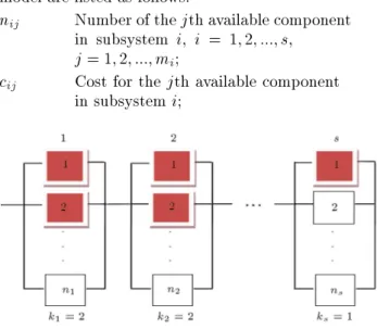
In this section, a RAP for a system as series-parallel with k-out-of-n subsystems demonstrated in Figure 1 is studied, in which mixed strategies can be chosen for each subsystem. The basic assumptions of the proposed problem are listed as follows.
2.1. Problem assumptions
System components are binary states (working or failed);
The components' failure rates are time dependent based on the Weibull distribution;
The redundancy strategy is mixed;
Each subsystem is working as k-out-of-n;
System components are non-repairable;
The failed components will not damage the whole system;
All parameters for components, including costs, weights, etc., are deterministic.
2.2. Notations of the model
The variables and parameters used in the mathematical model are listed as follows.
nij Number of the jth available component
in subsystem i, i = 1; 2; :::; s, j = 1; 2; :::; mi;
cij Cost for the jth available component
in subsystem i;
Table 1. A summary of literature review.
Authors Failure rates Description Solving method
Fye et al.
(1968) Constant Presented RAP for the rst time Dynamic programming Nakagawa and
Miyazaki (1981) Constant Model of Modied Fye et al. Surrogate constraint
Misra and
Sharma (1991) Constant
Considered a series-parallel system with k-out-of-n subsystems under
active redundancy policy
Zero-one programming
Pham
(1992) Constant
Proposed RAP for systems with a single k-out-of-n subsystem
under active redundancy
Mathematical and statistical relations
Pham and
Malon (1994) Constant
Considered multi-failure
mode for components in Pham (1992) Mathematical and statistical relations Chern
(1992) Constant Proved that RAP is Np-hard Mathematical and statistical relations Ida et al.
(1994) Constant
Proposed RAP of series-parallel systems
with multiple failure state components Genetic algorithm Painton and
Campbell (1995) Constant Presented a series-parallel RAP under risk Genetic algorithm Coit and
Liu (2000) Constant
Proposed RAP with k-out-of-n subsystems
under active and cold-standby redundancy Zero-one integer programming Coit
(2003) Constant
Considered redundancy strategy as a
decision variable for Coit and Liu (2000) Integer programming
Tavakkoli-Moghaddam
et al. (2008) Constant
Assumed that, the redundancy strategy for each subsystem is predetermined and xed
(active or cold-standby)
Genetic algorithm
Keshavarz Ghorabaee
et al. (2015) Constant
Presented BORAP for a system with k-out-of-n
subsystems and non-identical components Genetic algorithm and NSGA-II Zhang and
Chen (2016) Constant
Worked on reliability redundancy allocation
problems modeled in an interval environment Particle swarm optimization algorithm Teimouri et al.
(2016) Constant Developed an electromagnetism to solve RAP Memory-based electromagnetism-likemechanism algorithm Pourkarim Guilani
et al. (2017) Constant
Proposed MORAP for three-state systems
Table 1. A summary of literature review (continued).
Authors Failure rates Description Solving method
Garg et al.
(2014) General Presented a BORAP in fuzzy environment Swarm optimization Garg et al.
(2014) General Provided a MORAP in fuzzy environment
Genetic algorithm and particle swarm optimization
Garg (2015) General Proposed a RRAP under the various
nonlinear resource constraints Biogeography based optimization Garg
(2015) General
Presented a RRAP with nonlinear
resource constraints Cuckoo search Ardakan and
Hamadani (2014) Constant
Proposed RAP with the mixed
redundancy strategy Genetic algorithm Ardakan et al.
(2015) Constant
Proposed MORAP with the mixed
redundancy strategy NSGA-II
Gholinezhad and
Hamadani (2017) Constant
Proposed RAP in which the redundancy strategy (active, cold standby, or mixed)
is considered as a decision variable
Genetic algorithm
Nourelfath et al.
(2012) Constant
Used Markov and UGF to obtain
multi-state system reliability Genetic algorithm and Tabu search Pourkarim Guilani
et al. (2014) Constant
Used Markov to obtain reliability function of
three-state systems Dierential equations Kim and Kim
(2017) Constant
Proposed a new Markov chain
approach for standby RRAP Genetic algorithm Chang and Kuo
(2018) Constant
Considered generalized redundancy
allocation problem Simulation-based optimization Azimi et al.
(2017) Time-dependent
Proposed a non-exponential redundancy
allocation problem in k-out-of-n systems Meta-heuristic and simulation Ardakan et al.
(2017) & ConstantTime-dependent
The reliability of components considered
as a function of time Genetic algorithm Pourkarim Guilani
et al. (2016) Time-dependent
Used simulation to obtain reliability function as implicit
Genetic algorithm and random search
Current paper Time-dependent Used simulation to obtain reliability
wij Weight for the jth available component
in subsystem i;
ki The minimum requirement amount of
components that must be working in each subsystem (n k);
na
ij Number of the jth available component
in subsystem i working as active; nc
ij Number of the jth available component
in subsystem i working as cold-standby; nmax;i The upper bound on the assigned
number of components in subsystem i; zij A binary variable equals 1 if the
jth available component is placed in subsystem i and zero otherwise; A Shape parameters of the Weibull
distribution;
B Scale parameters of the Weibull distribution;
t Mission time. 2.3. Mathematical model
The optimization model of the redundancy allocation problem is presented as follows:
MaxR =Ys
i=1
f(nij; naij; ncij; zij; t; ); (1)
s.t.: n X i=1 mi X j=1
cijnij C; (2)
n X i=1 mi X j=1
wijnij W; (3)
nij zijnmax;i 8i = 1; :::; s; 8j = 1; :::; mi; (4) mi
X
j=1
zij= 1 8i = 1; :::; s; (5)
nc
ij= nij naij 8i = 1; :::; s; 8j = 1; :::; mi;
(6) ki naij nij 8i = 1; :::; s; 8j = 1; :::; mi; (7)
zij2 f0; 1g ; (8)
na
ij; ncij; nij 2 int: (9)
Eq. (1) is the objective function of the model which maximizes the system reliability. This function is obtained via the simulation replications as implicit for each subsystem based on several variables and pa-rameters such as the number of available components,
the number of components working in active and cold-standby modes, the type of selected components in subsystems, the mission time, and the error () asso-ciated with estimating this function via the simulation technique. Finally, the reliability of system is obtained by multiplication of subsystem reliabilities. As previ-ously mentioned, the components' failure rates are time dependent; therefore, calculating the system reliability is not an easy task. Thus, a simulation model is used to estimate the objective function. Inequalities (2) and (3) are cost and weight constraints, respectively. Constraint (4) puts an upper bound on the number of components of the subsystems if the jth available component is placed in subsystem i. Relation (5) ensures that there will be one type of components in each subsystem. In addition, Constraints (6)-(9) represent the conditions on model variables.
3. Simulation
In this section, a brief description of the Weibull distribution is provided. Then, the simulation steps are explained.
3.1. Weibull distribution
Weibull is one of the continuous probability distribu-tions that has been widely used in modeling of system reliability. Time-dependent failure rates of system components can be modeled properly through this distribution. The hazard function of this distribution is h(t) = AtB. This hazard function can be used for both
Increasing Failure Rate (IFR) and Decreasing Failure Rate (DFR) of system components so that if A > 0 and B > 0, then the hazard function is equal to an increasing function of t (the distribution is proper for modeling of the systems with IFR); if A > 0 and B < 0, then the hazard function is equal to an decreasing function of t (the distribution is proper for modeling of the systems with DFR) [29]. If the failure rates during time are considered as in the following function:
h(t) = BA
t A
B 1
; B > 0; A > 0; t 0; (10) then this hazard function belongs to the Weibull distribution; thus, its relationships such as reliability function, cumulative distribution function, and proba-bility distribution function are calculated as follows:
R (t) = e
t
R
y=0h(y):dy= e t
R
y=0 B
A(Ay)B 1:dy
= e
t/AB
; B > 0; A > 0; t 0; (11)
F (t)=1 e
t/AB
; B > 0; A > 0; t 0; (12)
f (t) = R (t) h (t) = BA
t A
B 1
e
t/AB
;
B > 0; A > 0; t 0: (13) In all of the above equations, B is the shape parameter, and A is the scale parameter of the Weibull distribu-tion. In order to see further studies on the Weibull distribution, [30,31] are recommended.
3.2. Simulation implementation
As previously mentioned, the simulation has been always used to calculate reliability function of a sub-system with time-dependent components, explicitly. Therefore, the reliability function for a subsystem via simulation is estimated; then, the estimated function will be used for the whole system reliability. Since the redundancy policy is considered as the mixed one for a k-out-of-n system, number of components (n), min-imum number of requirement component (k), number of active components (na), and number of cold-standby
components (nc) of each subsystem are required during
each iteration of the simulation process. Because these variables are dependent on each other, in order to satisfy this dependency and create feasible designs for simulation, two new auxiliary variables are dened as follows: k0and na0
, both of which are between 0 and 1. We know that in a k-out-of-n system, the amount of k should be between 1 and n (1 k n). In addition, k value is between 1 and n at all experiment levels; thus, it can be derived from Eq. (14):
k = round (1 + k0 (n 1)) : (14)
According to Eq. (14), for dierent values of k0between
0 and 1, k can be between 1 and n. In addition, we know that in a k-out-of-n system, at least k components should work actively. Therefore, in each subsystem, we will have k na n. Therefore, for dierent values of
na0
between 0 and 1, nais between k and n in Eq. (15):
na= round k + na0 (n k): (15)
Then, the number of cold-standby components in each subsystem is calculated by nc = n na. The pseudo
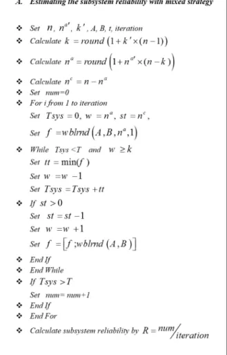
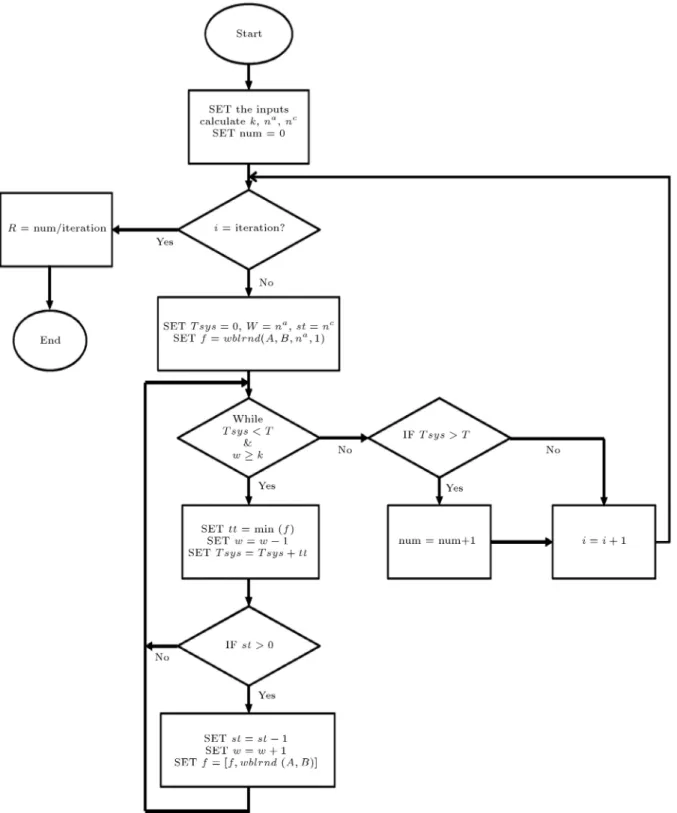
code and the owchart of simulation are shown in Figures 2 and 3, respectively, and all the steps involved in the simulation experiments are coded in MATLAB 10 software.
As shown in Figures 2 and 3, details of the simu-lation experiments are described as follows. At rst, the input parameters are added. These parameters include n, na0
, k0, A, B, and t. Then, by Eqs. (14)
and (15), the values of na and k are obtained. Then,
for each iteration, a number of the components working as active are inserted in w, and a number of the components reserved as cold-standby are inserted in st.
Figure 2. Pseudo code of simulation experiments.
In addition, random numbers are generated based on the Weibull distribution with parameters A and B for the number of active components and are inserted in f. In the simulation process, (T sys) is the life time of the given subsystem. In this process, if T sys > t, the given subsystem is working safely and there is no problem. However, when T sys < t, it means that the system needs to be investigated. Indeed, when T sys < t, the system performance has a problem that must be eliminated. While the subsystem life time (T sys) is less than t and w is more than k, the minimum amount of f will be selected. This amount eliminates f and adds to T sys. Therefore, one of the active working objects is reduced. Now, one of the cold-standby components will be deleted from st and added to w. To put it more delicately, if there is at least one component as reserved, this component enters the circuit. At the same time, a random number is generated based on the Weibull distribution with parameters A and B, and this number joins the existing values of set f.
This procedure continues until w < k, and there are some cold-standby components marked as reserved. In addition, if T sys > t, it means that the subsystem works safely. At the end, the subsystem reliability
Figure 3. Flowchart of simulation experiments.
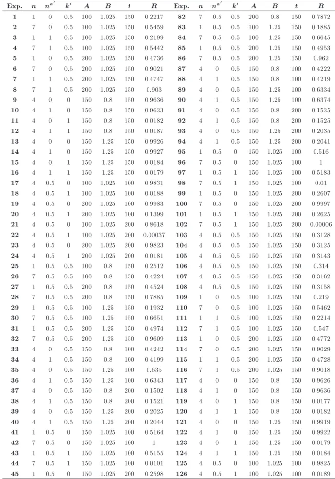
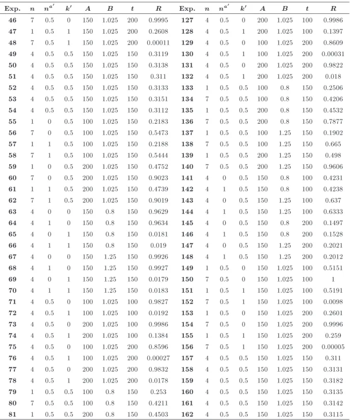
is estimated as the number of running loop processes divided by the number of iterations (num/iter). 3.3. Experiments of simulation
To estimate the objective function of the mathemat-ical model presented in Section 2, it is required to conduct several experiments. For this purpose, a Box-Behnken design is performed in order to create
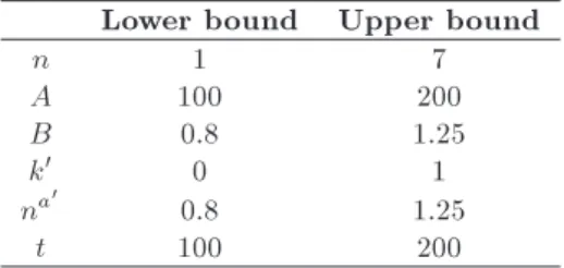
dierent scenarios to estimate the reliability function in MINITAB 16 software. Here, six factors are considered in each scenario. The factor levels considered in the simulation experiments are demonstrated in Table 2, most of which have been adopted from Pourkarim Guilani et al. [29]. In addition, six central points were added in order to test a possible curvature involved in the response function. Moreover, the number of
Table 2. The lower and upper bounds of input parameters for numerical examples.
Lower bound Upper bound
n 1 7
A 100 200
B 0.8 1.25
k0 0 1
na0
0.8 1.25
t 100 200
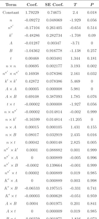
replications is 30 for each design. The values of factors in each experiment and their results are shown in Table 3. Moreover, the estimated regression coecients for reliability function of a subsystem are provided in Table 4. In all designs, R sq = 91:46%, showing that the results are reliable.
According to the results in Table 3, the subsystem reliability function is estimated by implementing a non-linear regression in MINITAB 16 software as Eq. (16):
R =1:79229 0:09272 n 0:17104 na0
0:48286 k0 0:01287 A 1:04362
B + 0:00468 t + 0:00695n n+0:16938 na0 na0+ 0:42872 k0 k0+ 0:00005
A A + 0:69108 B B 0:00002 t t 0:00002 n na0 0:16599
n k0+ 0:00015 n A + 0:08017
n B + 0:00042 n t + 0:00010 na0
k0 0:00020 na0 B + 0:00002 na0
t 0:06533 k0 B 0:00003 k0
t + 0:00040 A B 0:00359 B t: (16) Therefore, Eq. (16) resulting from the simulation repli-cations is used as the objective function (reliability function) in the mathematical model of the problem. The solution methodology will be presented in the next section.
4. Solution methodology
The presented model in Section 3 is an Integer Non-linear Programming Model (INLP), and solving this problem via exact method is impossible [6]. However, it is possible to transform the problem to an Integer Linear Programming (ILP) based on [10]. Thus, the problem is linearized by taking the logarithm of the
objective function to provide conditions to apply in-teger programming algorithms. Some new parameters and variables are dened in the following in order to change variables of the rst RAP model, presented in Subsection 2.3.
p An index that takes value between ki
and nmax;i;
aijp The cost of deployment p components
of type j in subsystem i; bijp The weight of deployment p
components of type j in subsystem i; ijpq Logarithm of the reliability of p
components of type j in subsystem i, in which q components are active and p q components are cold-standby; yijpq A binary variable equals 1 if p
components of type j used in subsystem i and zero otherwise, in which q components are active and p q components are cold-standby.
In addition, aijp, bijp, and ijpq are expressed
as functions of specied components and problem parameters. These values are obtained as follows:
aijp= cij p 8i = 1; :::; s;
8j = 1; :::; mi 8p = ki; :::; nmax;i; (17)
bijp= wij p 8i = 1; :::; s;
8j = 1; :::; mi 8p = ki; :::; nmax;i; (18)
ijpq= LnRsim(p; q; p q; zij; t)
8i = 1; :::; s; 8j = 1; :::; mi;
8p = ki; :::; nmax;i; 8q = ki; :::; p: (19)
Finally, the new ILP is formed as follows: Max R =Xs
i=1 mi
X
j=1 nXmax;i
p=ki
p
X
q=ki
ijpqyijpq;
s.t. s X i=1 mi X j=1 nXmax;i
p=ki
p
X
q=ki
aijpyijpq C;
s X i=1 mi X j=1 nXmax;i
p=ki
p
X
q=ki
bijpyijpq W;
mi
X
j=1 nXmax;i
p=ki
p
X
q=ki
yijpq= 1 8i = 1; :::; s;
Table 3. Experimental results obtained via simulation.
Exp. n na0 k0 A B t R Exp. n na0 k0 A B t R
1 1 0 0.5 100 1.025 150 0.2217 82 7 0.5 0.5 200 0.8 150 0.7872 2 7 0 0.5 100 1.025 150 0.5459 83 1 0.5 0.5 100 1.25 150 0.1885 3 1 1 0.5 100 1.025 150 0.2199 84 7 0.5 0.5 100 1.25 150 0.6645 4 7 1 0.5 100 1.025 150 0.5442 85 1 0.5 0.5 200 1.25 150 0.4953 5 1 0 0.5 200 1.025 150 0.4736 86 7 0.5 0.5 200 1.25 150 0.962
6 7 0 0.5 200 1.025 150 0.9021 87 4 0 0.5 150 0.8 100 0.4222
7 1 1 0.5 200 1.025 150 0.4747 88 4 1 0.5 150 0.8 100 0.4219
8 7 1 0.5 200 1.025 150 0.903 89 4 0 0.5 150 1.25 100 0.6334
9 4 0 0 150 0.8 150 0.9636 90 4 1 0.5 150 1.25 100 0.6374
10 4 1 0 150 0.8 150 0.9633 91 4 0 0.5 150 0.8 200 0.1535
11 4 0 1 150 0.8 150 0.0182 92 4 1 0.5 150 0.8 200 0.1525
12 4 1 1 150 0.8 150 0.0187 93 4 0 0.5 150 1.25 200 0.2035
13 4 0 0 150 1.25 150 0.9926 94 4 1 0.5 150 1.25 200 0.2041
14 4 1 0 150 1.25 150 0.9927 95 1 0.5 0 150 1.025 100 0.516
15 4 0 1 150 1.25 150 0.0184 96 7 0.5 0 150 1.025 100 1
16 4 1 1 150 1.25 150 0.0179 97 1 0.5 1 150 1.025 100 0.5183
17 4 0.5 0 100 1.025 100 0.9831 98 7 0.5 1 150 1.025 100 0.01
18 4 0.5 1 100 1.025 100 0.0188 99 1 0.5 0 150 1.025 200 0.2607 19 4 0.5 0 200 1.025 100 0.9983 100 7 0.5 0 150 1.025 200 0.9997 20 4 0.5 1 200 1.025 100 0.1399 101 1 0.5 1 150 1.025 200 0.2625 21 4 0.5 0 100 1.025 200 0.8618 102 7 0.5 1 150 1.025 200 0.00006 22 4 0.5 1 100 1.025 200 0.00037 103 4 0.5 0.5 150 1.025 150 0.3128 23 4 0.5 0 200 1.025 200 0.9823 104 4 0.5 0.5 150 1.025 150 0.3125 24 4 0.5 1 200 1.025 200 0.0181 105 4 0.5 0.5 150 1.025 150 0.3143 25 1 0.5 0.5 100 0.8 150 0.2512 106 4 0.5 0.5 150 1.025 150 0.314 26 7 0.5 0.5 100 0.8 150 0.4224 107 4 0.5 0.5 150 1.025 150 0.3162 27 1 0.5 0.5 200 0.8 150 0.4524 108 4 0.5 0.5 150 1.025 150 0.3158 28 7 0.5 0.5 200 0.8 150 0.7885 109 1 0 0.5 100 1.025 150 0.219 29 1 0.5 0.5 100 1.25 150 0.1932 110 7 0 0.5 100 1.025 150 0.5462 30 7 0.5 0.5 100 1.25 150 0.6651 111 1 1 0.5 100 1.025 150 0.2214 31 1 0.5 0.5 200 1.25 150 0.4974 112 7 1 0.5 100 1.025 150 0.547 32 7 0.5 0.5 200 1.25 150 0.9609 113 1 0 0.5 200 1.025 150 0.4772
33 4 0 0.5 150 0.8 100 0.4242 114 7 0 0.5 200 1.025 150 0.9029
34 4 1 0.5 150 0.8 100 0.4199 115 1 1 0.5 200 1.025 150 0.4728
35 4 0 0.5 150 1.25 100 0.635 116 7 1 0.5 200 1.025 150 0.9018
36 4 1 0.5 150 1.25 100 0.6343 117 4 0 0 150 0.8 150 0.9626
37 4 0 0.5 150 0.8 200 0.1502 118 4 1 0 150 0.8 150 0.9636
38 4 1 0.5 150 0.8 200 0.1521 119 4 0 1 150 0.8 150 0.0177
39 4 0 0.5 150 1.25 200 0.2025 120 4 1 1 150 0.8 150 0.0182
40 4 1 0.5 150 1.25 200 0.2044 121 4 0 0 150 1.25 150 0.9919
41 1 0.5 0 150 1.025 100 0.5164 122 4 1 0 150 1.25 150 0.9922
42 7 0.5 0 150 1.025 100 1 123 4 0 1 150 1.25 150 0.0179
43 1 0.5 1 150 1.025 100 0.5155 124 4 1 1 150 1.25 150 0.0184
44 7 0.5 1 150 1.025 100 0.0101 125 4 0.5 0 100 1.025 100 0.9825 45 1 0.5 0 150 1.025 200 0.2598 126 4 0.5 1 100 1.025 100 0.0189
Table 3. Experimental results obtained via simulation (continued). Exp. n na0
k0 A B t R Exp. n na0
k0 A B t R
46 7 0.5 0 150 1.025 200 0.9995 127 4 0.5 0 200 1.025 100 0.9986 47 1 0.5 1 150 1.025 200 0.2608 128 4 0.5 1 200 1.025 100 0.1397 48 7 0.5 1 150 1.025 200 0.00011 129 4 0.5 0 100 1.025 200 0.8609 49 4 0.5 0.5 150 1.025 150 0.3119 130 4 0.5 1 100 1.025 200 0.00031 50 4 0.5 0.5 150 1.025 150 0.3138 131 4 0.5 0 200 1.025 200 0.9822 51 4 0.5 0.5 150 1.025 150 0.311 132 4 0.5 1 200 1.025 200 0.018 52 4 0.5 0.5 150 1.025 150 0.3133 133 1 0.5 0.5 100 0.8 150 0.2506 53 4 0.5 0.5 150 1.025 150 0.3151 134 7 0.5 0.5 100 0.8 150 0.4206 54 4 0.5 0.5 150 1.025 150 0.3112 135 1 0.5 0.5 200 0.8 150 0.4532 55 1 0 0.5 100 1.025 150 0.2183 136 7 0.5 0.5 200 0.8 150 0.7877 56 7 0 0.5 100 1.025 150 0.5473 137 1 0.5 0.5 100 1.25 150 0.1902 57 1 1 0.5 100 1.025 150 0.2188 138 7 0.5 0.5 100 1.25 150 0.665 58 7 1 0.5 100 1.025 150 0.5444 139 1 0.5 0.5 200 1.25 150 0.498 59 1 0 0.5 200 1.025 150 0.4752 140 7 0.5 0.5 200 1.25 150 0.9606
60 7 0 0.5 200 1.025 150 0.9023 141 4 0 0.5 150 0.8 100 0.4231
61 1 1 0.5 200 1.025 150 0.4739 142 4 1 0.5 150 0.8 100 0.4238
62 7 1 0.5 200 1.025 150 0.9019 143 4 0 0.5 150 1.25 100 0.637
63 4 0 0 150 0.8 150 0.9629 144 4 1 0.5 150 1.25 100 0.6333
64 4 1 0 150 0.8 150 0.9634 145 4 0 0.5 150 0.8 200 0.1497
65 4 0 1 150 0.8 150 0.0181 146 4 1 0.5 150 0.8 200 0.1528
66 4 1 1 150 0.8 150 0.019 147 4 0 0.5 150 1.25 200 0.2021
67 4 0 0 150 1.25 150 0.9926 148 4 1 0.5 150 1.25 200 0.2012
68 4 1 0 150 1.25 150 0.9927 149 1 0.5 0 150 1.025 100 0.5151
69 4 0 1 150 1.25 150 0.0179 150 7 0.5 0 150 1.025 100 1
70 4 1 1 150 1.25 150 0.0183 151 1 0.5 1 150 1.025 100 0.5191
71 4 0.5 0 100 1.025 100 0.9827 152 7 0.5 1 150 1.025 100 0.0098 72 4 0.5 1 100 1.025 100 0.0192 153 1 0.5 0 150 1.025 200 0.2601 73 4 0.5 0 200 1.025 100 0.9986 154 7 0.5 0 150 1.025 200 0.9996 74 4 0.5 1 200 1.025 100 0.1384 155 1 0.5 1 150 1.025 200 0.259 75 4 0.5 0 100 1.025 200 0.8596 156 7 0.5 1 150 1.025 200 0.00005 76 4 0.5 1 100 1.025 200 0.00027 157 4 0.5 0.5 150 1.025 150 0.311 77 4 0.5 0 200 1.025 200 0.9832 158 4 0.5 0.5 150 1.025 150 0.3131 78 4 0.5 1 200 1.025 200 0.0178 159 4 0.5 0.5 150 1.025 150 0.3182 79 1 0.5 0.5 100 0.8 150 0.253 160 4 0.5 0.5 150 1.025 150 0.3135 80 7 0.5 0.5 100 0.8 150 0.4211 161 4 0.5 0.5 150 1.025 150 0.3142 81 1 0.5 0.5 200 0.8 150 0.4503 162 4 0.5 0.5 150 1.025 150 0.3115
Since the second model is linear and is in the form of a standard zero-one integer programming, there are several algorithms to solve it exactly. In this paper, a Branch and Bound (B&B), as an exact algorithm, is used to solve the proposed model based on [10].
Of course, it is worth mentioning that in large-scale problems where integer programming approaches
are inecient, heuristic and meta-heuristic approaches are the best ways to achieve the near-optimum solutions.
5. Numerical example
Table 4. Estimated regression coecients for R.
Term Coef. SE Coef. T P
Constant 1.79229 0.74675 2.4 0.018 n -0.09272 0.048069 -1.929 0.056 na0
-0.17104 0.261405 -0.654 0.514 k0 -0.48286 0.282734 -1.708 0.09
A -0.01287 0.00347 -3.71 0 B -1.04362 0.916778 -1.138 0.257
t 0.00468 0.003481 1.344 0.181 n n 0.00695 0.002177 3.193 0.002 na0 na0 0.16938 0.078386 2.161 0.032
k0 k0 0.42872 0.078386 5.469 0
A A 0.00005 0.000008 5.981 0 A B 0.69108 0.387093 1.785 0.076
t t -0.00002 0.000008 -1.927 0.056 n na0
-0.00002 0.014814 -0.002 0.999 n k0 -0.16599 0.014814 -11.205 0
n A 0.00015 0.000105 1.431 0.155 n B 0.08017 0.032919 2.435 0.016 n t 0.00042 0.000148 2.825 0.005 na0
k0 0.0001 0.088882 0.001 0.999
na0
A 0 0.000889 -0.005 0.996
na0 B -0.0002 0.139664 -0.001 0.999
na0
t 0.00002 0.000889 0.019 0.985 K0 A 0 0.000889 0.003 0.998
K0 B -0.06533 0.197515 -0.331 0.741
K0 t -0.00003 0.000628 -0.051 0.959
A B 0.0004 0.001975 0.201 0.841
A t 0 0.000009 0.019 0.985
B t -0.00359 0.001975 -1.816 0.072
S = 0:108858, P RESS = 2:40531, R Sq = 91:46%, R Sq(pred) = 87:06%, R Sq(adj) = 89:73%.
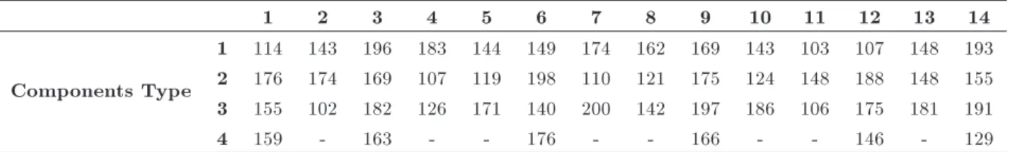
demonstrate the verication of the proposed method-ology. A system with 14 subsystems is considered, in which the subsystems are connected serially to each other. The input parameters of the model are taken
from [29]. The number of available types of components and the minimum requirement amount of components, which have to be working in each subsystem, are provided in Table 5. Moreover, the two parameters of the Weibull distribution of the available components in each subsystem are demonstrated in Tables 6 and 7. The cost and weight of each component are presented in Tables 8 and 9, respectively. In addition, the switch reliability is 1.
In addition, the maximum cost for the system is 300, the maximum system weight is 400, and the upper bound on the assigned number of components in each subsystem (nmax i) is 5. In this system, the mixed
strategy for each redundancy is used. The number of decision variables for the second model of this system is obtained from Eq. (20).
=Ys
i=1
mi(nmax;i ki+ 1)2: (20)
Therefore, the total exact number of feasible and infeasible solutions is 2.
The problem is coded in MATLAB 10, and a Pentium IV computer with a core 2 CPU 2.4 GHz and 3 GB RAM under Windows 7 operating system is used in order to run the program. After solving the problem using a B&B algorithm, the results are summarized in Table 10.
In this table, the rst column presents the type of selective component; the second column indicates the number of selective component in each subsystem. The third and fourth columns show the number of active and cold-standby components in each subsystem, respectively. Moreover, according to Table 10, the system reliability is 0.4779. In addition, sensitivity analysis has been carried out in order to investigate the eect of the number of components in each subsystem (nmax i) on reliability function. For this purpose, 10
test problems are used to study the sensitivity analysis while keeping the other parameters stable, and the results are listed in Table 11 and Figure 4. As results show, any increase in nmax;i leads to an increase in
system reliability, which shows a rational fact.
6. Conclusion and future researches
In many real-world systems, the components do not have a constant failure rate. Indeed, the components' failure rates change occasionally. Therefore, systems with time-dependent failure rates are considered more
Table 5. Number of available components for each subsystem.
i 1 2 3 4 5 6 7 8 9 10 11 12 13 14
m 4 3 4 3 3 4 3 3 4 3 3 4 3 4
Table 6. The scale parameter (A) of the Weibull distribution for each type of components in each subsystem.
1 2 3 4 5 6 7 8 9 10 11 12 13 14
Components Type
1 114 143 196 183 144 149 174 162 169 143 103 107 148 193 2 176 174 169 107 119 198 110 121 175 124 148 188 148 155 3 155 102 182 126 171 140 200 142 197 186 106 175 181 191
4 159 - 163 - - 176 - - 166 - - 146 - 129
Table 7. The shape parameter (B) of the Weibull distribution for each type of components in each subsystem.
1 2 3 4 5 6 7 8 9 10 11 12 13 14
Components Type
1 1.07 1.04 0.85 0.95 1.17 0.83 0.89 1.05 1.13 1.12 1.24 1.16 1.04 1.22 2 0.94 1.21 0.83 1.14 0.89 1.08 1.07 1.22 1.01 1.17 1 1.17 1.05 1.22 3 1.23 1.16 1.13 1.23 1.22 1.17 1 0.84 1.17 0.94 0.99 1.04 1.22 1.16
4 1.17 - 1.16 - - 0.96 - - 1.09 - - 1.21 - 1.22
Table 8. The cost of each type of components in each subsystem.
1 2 3 4 5 6 7 8 9 10 11 12 13 14
Components Type
1 1 2 2 3 2 3 4 3 2 4 3 2 2 4
2 1 1 3 4 2 3 4 5 3 4 4 3 3 4
3 2 1 1 5 3 2 5 6 4 5 5 4 2 5
4 2 - 4 - - 2 - - 3 - - 5 - 6
Table 9. The weight of each type of components in each subsystem.
1 2 3 4 5 6 7 8 9 10 11 12 13 14
Components Type
1 3 8 7 5 4 5 7 4 8 6 5 4 5 6
2 4 10 5 6 3 4 8 7 9 5 6 5 5 7
3 2 9 6 4 5 5 9 6 7 6 6 6 6 6
4 5 - 4 - - 4 - - 8 - - 7 - 9
Table 10. The results of the numerical example. i zi ni nai nci
1 3 5 5 0
2 2 5 2 3
3 3 5 2 3
4 1 5 2 3
5 3 5 2 3
6 2 5 2 3
7 3 5 2 3
8 1 5 5 0
9 3 5 2 3
10 3 5 2 3
11 1 5 5 0
12 2 5 2 3
13 3 5 2 3
14 1 5 2 3
realistic. The Weibull probability distribution is one of the proper distributions to model the time-dependent failure rates. Due to its hazard function, it has appropriate exibility to model time-dependent failure rates and can be used in many real-world systems.
Figure 4. A graphical comparison to investigate eect of nmax;ion system reliability via 10 test problems.
This suitable property of the Weibull distribution can overcome the limitation of previous studies in which the component failure rates were considered as constant based on exponential distribution. This research study investigated a RAP under k-out-of-n subsystems with time-dependent failure rates based on this distribution. Moreover, it was assumed that the redundancy strategy was mixed. Since it is hard to obtain the reliability
Table 11. The results of test problems to investigate eect of nmax;ion system reliability .
i
1 2 3 4 5 6 7 8 9 10 11 12 13 14 R
Test problems
1 3 5 5 5 5 5 5 5 5 5 5 5 5 5 0.254
2 4 5 5 5 5 5 5 5 5 5 5 5 5 5 0.3764
3 5 5 5 5 5 5 5 5 5 5 5 5 5 5 0.4779
4 6 5 5 5 5 5 5 5 5 5 5 5 5 5 0.5468
5 7 5 5 5 5 5 5 5 5 5 5 5 5 5 0.6214
6 7 6 5 5 5 5 5 5 5 5 5 5 5 5 0.6822
7 7 7 5 5 5 5 5 5 5 5 5 5 5 5 0.7222
8 7 7 6 5 5 5 5 5 5 5 5 5 5 5 0.8042
9 7 7 7 5 5 5 5 5 5 5 5 5 5 5 0.8654
10 7 7 7 6 5 5 5 5 5 5 5 5 5 5 0.9764
function of such systems explicitly, a simulation-based optimization approach was developed to estimate the system reliability function. Then, due to the Np-hardness of the proposed RAP, the original INLP was replaced by an ILP problem. Finally, a B&B algorithm was developed to solve the ILP model exactly. In addition, a numerical illustration was presented to demonstrate the application of the proposed method-ology. The presented idea in this paper can help man-agers and owners of electronic and mechanical systems make better decisions on their systems according to real-world issues and not merely based on academic assumptions. For future researches in this area, the following lines are recommended:
Considering other probability distributions such as normal, lognormal, Gumbel, log-logistic, etc. to model the systems component life;
Considering systems with failure rates which are dependent on working components;
Considering repairable components;
Considering failure rates of components as fuzzy variables;
Studying reliability evaluation of systems with time-dependent failure rate via mathematical and statis-tical relations.
References
1. Fye, D.E., Hines, W.W., and Lee, N.K. \System
reliability allocation and a computational algorithm", IEEE Transactions on Reliability, 17, pp. 64-69 (1968).
2. Nakagawa, Y. and Miyazaki, S. \Surrogate constraints
algorithm for reliability optimization problems with two constraints", IEEE Transactions on Reliability, 30, pp. 175-180 (1981).
3. Misra, K.B. and Sharma, U. \Reliability optimization
of a system by zero-one programming", Microelectron-ics and Reliability, 31, pp. 323-335 (1991).
4. Pham, H. \Optimal design of k-out-of-n redundant
systems", Microelectronics and Reliability, 32, pp. 119-126 (1992).
5. Pham, H. and Malon, D.M. \Optimal design of systems
with competing failure modes", IEEE Transactions on Reliability, 43, pp. 251-254 (1994).
6. Chern, M.S. \On the computational complexity of
reliability redundancy allocation in a series system", Operation Research Letters, 11, pp. 309-315 (1992).
7. Ida, K., Gen, M., and Yokota, T. \System
reliabil-ity optimization with several failure modes by ge-netic algorithm", Proceeding of the 16th International Conference on Computers and Industrial Engineering, Ashikaga of Japan (1994).
8. Painton, L. and Campbell, J. \Genetic algorithms in
optimization of system reliability", IEEE Transactions on Reliability, 44(2), pp. 172-178 (1995).
9. Coit, D.W. and Liu, J. \System reliability optimization
with k-out-of-n subsystems", International Journal of Reliability, Quality & Safety Engineering, 35, pp. 535-544 (2000).
10. Coit, D.W. \Maximization of system reliability with
a choice of redundancy strategies", IEEE Transaction on Reliability, 35, pp. 535-544 (2003).
11. Tavakkoli-Moghaddam, R., Safari, J., and Sassani,
F. \Reliability optimization of series-parallel systems with a choice of redundancy strategies using a genetic algorithm", Reliability Engineering and System Safety, 93, pp. 550-556 (2008).
12. Ghorabaee, M.K., Amiri, M., and Azimi, P. \Genetic
algorithm for solving bi-objective redundancy alloca-tion problem with k-out-of-n subsystems", Applied Mathematical Modelling, 39(20) pp. 6396-6409 (2015).
13. Zhang, E. and Chen, Q. \Multi-objective reliability
redundancy allocation in an interval environment using particle swarm optimization", Reliability Engineering & System Safety, 145, pp. 83-92 (2016).
14. Teimouri, M., Zaretalab, A, Niaki, S.T.A., and Shari, M. \An ecient memory-based electromagnetism-like mechanism for the redundancy allocation problem", Applied Soft Computing, 38, pp. 423-436 (2016).
15. Pourkarim Guilani, P., Niaki, S.T.A., Zaretalab, A.,
and Pourkarim Guilani, P. \A bi-objective model to optimize reliability and cost of three-state systems with k-out-of-n subsystems", Sciantia Iranica, 24(3), pp. 1585-1602 (2017).
16. Garg, H., Rani, M., Sharma, S.P., and Vishwakarma,
Y. \Bi-objective optimization of the reliability-redundancy allocation problem for series-parallel sys-tem", Journal of Manufacturing Systems, 33(3), pp. 335-347 (2014).
17. Garg, H., Rani, M., Sharma, S.P., and Vishwakarma,
Y. \Intuitionistic fuzzy optimization technique for solving multi-objective reliability optimization prob-lems in interval environment", Expert Systems with Applications, 41(7), pp. 3157-3167 (2014).
18. Garg, H. \An ecient biogeography based
optimiza-tion algorithm for solving reliability optimizaoptimiza-tion prob-lems", Swarm and Evolutionary Computation, 24, pp. 1-10 (2015).
19. Garg, H. \An approach for solving constrained
reliability-redundancy allocation problems using cuckoo search algorithm", Beni-Suef University Journal of Basic and Applied Sciences, 4(1), pp. 14-25 (2015).
20. Ardakan, M.A. and Hamadani, A.Z. \Reliability
opti-mization of series-parallel systems with mixed redun-dancy strategy in subsystems", Reliability Engineering and System Safety, 130, pp. 132-139 (2014).
21. Ardakan, M.A., Hamadani, A.Z., and Alinaghian,
M. \Optimizing bi-objective redundancy allocation problem with a mixed redundancy strategy", ISA Transactions, 55, pp. 116-128 (2015).
22. Gholinezhad, H. and Hamadani, A.Z. \A new model
for the redundancy allocation problem with component mixing and mixed redundancy strategy", Reliability Engineering & System Safety, 164, pp. 66-73 (2017).
23. Nourelfath, M., Ch^atelet, E., and Nahas, N. \Joint
redundancy and imperfect preventive maintenance optimization for series-parallel multi-state degraded systems", Reliability Engineering and System Safety, 103, pp. 51-60 (2012).
24. Pourkarim Guilani, P., Shari, M., Niaki, S.T.A., and
Zaretalab, A. \Reliability evaluation of non-reparable three-state systems using Markov model and its com-parison with the UGF and the recursive methods", Reliability Engineering and System Safety, 129, pp. 29-35 (2014).
25. Kim, H. and Kim, P. \Reliability-redundancy
alloca-tion problem considering optimal redundancy strategy using parallel genetic algorithm", Reliability Engineer-ing and System Safety, 159, pp. 153-160 (2017).
26. Chang, K.H. and Kuo, P.Y. \An ecient simulation
optimization method for the generalized redundancy
allocation problem", European Journal of Operational Research, 265(3), pp. 1094-1101 (2018).
27. Azimi, P., Hemmati, M., and Chambari, A.
\Solv-ing the redundancy allocation problem of k-out-of-n with non-exponential repairable components using op-timization via simulation approach", Scientia Iranica, 24(3), pp. 1547-1560 (2017).
28. Ardakan, M.A., Mirzaei, Z., Hamadani, A.Z., and
Elsayed, E.A. \Reliability optimization by considering time-dependent reliability for components", Quality and Reliability Engineering International, 33(8), pp. 1641-1654 (2017).
29. Pourkarim Guilani, P., Azimi, P., Niaki, S.T.A., and
Niaki, S.A.A. \Redundancy allocation problem of a system with increasing failure rates of components based on Weibull distribution: A simulation-based optimization approach", Reliability Engineering and System Safety, 152, pp. 187-196 (2016).
30. Garg, H., Sharma, S.P., and Rani, M. \Behavior
analysis of pulping unit in a paper mill with Weibull fuzzy distribution function using ABCBLT technique", International Journal of Applied Mathematics and Mechanics, 8(4), pp. 86-96 (2012).
31. Garg, H., Sharma, S.P., and Rani, M. \Weibull fuzzy
probability distribution for analysing the behaviour of pulping unit in a paper industry", International Journal of Industrial and Systems Engineering, 14(4), pp. 395-413 (2013).
Biographies
Pedram Pourkarim Guilani is a PhD Candidate at the Faculty of Industrial and Mechanical Engineering in Qazvin Islamic Azad University, Qazvin, Iran. He holds BSc and MSc degrees, both in Industrial En-gineering from Qazvin Islamic Azad University. His areas of interest include reliability theory, optimization via simulation, meta-heuristic algorithms, and Markov theory.
Parham Azimi is an Associate Professor at the Faculty of Industrial and Mechanical Engineering in Qazvin Islamic Azad University, Qazvin, Iran. He has graduated in Industrial Engineering at Sharif Univer-sity of Technology, Tehran, Iran (BSc, MSc, and PhD). His areas of interest include simulation modeling, optimization via simulation, meta-heuristic algorithms, graph theory, AGV based material handling systems, reliability theory, and queue theory.
Mani Shari is an Assistant Professor at the Faculty of Industrial and Mechanical Engineering in Qazvin Islamic Azad University, Qazvin, Iran. He holds a BSc degree from Qazvin Islamic Azad University, MSc degree from South Tehran Branch, Islamic Azad University, and PhD degree from Tehran Research and
Science Islamic Azad University in Industrial Engineer-ing. His areas of interest include reliability engineering, combinatorial optimization, statistical optimization, and fuzzy set theory.
Maghsoud Amiri is a Professor at the Department of Industrial Management of Allameh Tabataba'i Uni-versity, Tehran, Iran. He has received PhD degree in
Industrial Engineering from Sharif University of Tech-nology, Tehran, Iran. He has published many papers in leading international journals. His research interests include multi-criteria decision-making (MCDM), data envelopment analysis (DEA), design of experiments (DOE), response surface methodology (RSM), fuzzy MCDM, inventory control, supply chain management, simulation and reliability engineering.