Evaluating alternative MPS development methods using MCDM
and numerical simulation
Negin Najafian1, M. M. Lotfi 1* 1
Department of Industrial Engineering, Faculty of Engineering, Yazd University, Yazd, Iran [email protected]
Abstract
One of the key elements in production planning hierarchy is master production scheduling. The aim of this study is to evaluate and compare thirteen alternative MPS development methods, including multi-objective optimization as well as twelve heuristics, in different operating conditions for multi-product single-level capacity-constrained production systems. We extract six critical criteria from the previous related researches and employ them in a MCDM framework. The Shannon entropy is used to weight the criterion and TOPSIS is proposed for ranking the alternative methods. To be able to generalize the results, 324 cases considering different operating conditions are simulated. The results show that the most important criteria are instability and inventory/setup costs, respectively. A performance analysis of MPS development methods is reported that the heuristics provides better results than multi-objective optimization in many conditions. A sensitivity analysis for critical parameters is also provided. Finally, the proposed methodology is implemented in a wire & cable company. Keywords: Master production scheduling; Multi-criteria decision making; heuristics; TOPSIS; Shannon entropy, Numerical simulation.
1- Introduction and literature review
Master production scheduling (MPS) identifies which quantities of products expect to manufacture during the periods (Jonsson & Kjellsdotter, 2015). It plays an important role in a manufacturing planning and control system as it helps management to control the manufacturing resources and activities. Moreover, MPS is as a key link in a production planning and scheduling chain connecting the upstream aggregate production plans (APP) to the downstream schedules, especially material requirements planning (MRP.) Hence, inappropriate decisions on the MPS development method may lead to a bad implementation which ultimately causes an infeasible and nervous MRP and poor delivery schedules as well as inefficient feedback to APP. One must, thus, ensure that the developed MPS is good enough before it is released to the manufacturing system. But, in practice, where production environment is uncertain due to the forecast errors or capacity problems, the MPS development is no longer a simple task.
*Corresponding author
ISSN: 1735-8272, Copyright c 2017 JISE. All rights reserved
Journal of Industrial and Systems Engineering
Vol. 10, special issue on production and inventory, pp 73-90 Winter (February) 2017
The MPS development may be viewed as a multi-product single-level capacity-constrained lot-sizing problem. In this regard, various methods exist in the literature which can be used for MPS development. A given method is, hence, not necessarily the best in all the companies and conditions. Therefore, the key question is: which method is the best for any condition? Furthermore, many companies choose a method and use it for a long time; then, it is important to select a correct method. Due to the variety of MPS development methods with different characteristics and the unique features and conditions, e.g., available capacity, demand pattern, operating conditions, and alike, of each company, the use of some methods is usually better than the others.
Different models in the literature were formulated to optimize one or more criterion for the MPS development. Usually, the cost criterion is used to develop MPS. Jeunet & Jonard (2000) reported that cost and computational time are the traditional key criteria for evaluating the lot-sizing techniques. Herrera et al. (2015) proposed a mixed-integer programming model which aimed at providing a set of plans such that a compromise between production cost and production stability is ensured. Akhoondi & Lotfi (2016) proposed a cost-based optimization model and heuristic algorithm for MPS problems under controllable processing times and scenario-based demands. Gahm et al. (2014) presented a multi-criteria MPS approach to minimize the costs.
Another criterion, which was mostly referred, is the customer service level. Soares and Vieira (2009) proposed GA to solve the MPS problem using the conflicting criteria including the maximization of service level and efficient use of resources as well as the minimization of inventory levels. Supriyanto & Noche (2011) presented a multi-objective MPS by establishing a reasonable trade-off between the minimization of inventory as well as the maximization of customer satisfaction and resource utilization. Zhao & Xie (1998)investigated the performance of ten lot-sizing and freezing rules for MPS according to the total costs, schedule instability, and service level in an uncapacitated multi-item multi-level system. Results indicated that the selection of the lot-sizing rules significantly influenced the selection of parameters for freezing the MPS.
As mentioned, MPS, in practice, is influenced by the multiple conflicting objectives; e.g., the minimization of the costs and instability as well as the maximization of the customer service level and capacity utilization. In fact, it is clear that using the single objective models does not represent the reality to decision makers and the results may be impractical. For this reason, the researchers went to the use of the multiple criteria models.
However, for reaching the best solution to the MPS, not only paying attention to the main criteria is important, but also, selecting the best method by which appropriate MPS quantities are scheduled at the corresponding time horizon given the criteria subject to the prevailing constraints is critical. MPS, in turn, may be viewed as a capacitated multi-product single level lot-sizing & scheduling problem since it determines the quantity of finished products to be produced in each period of a mid-term horizon. So, we study the well-known lot-sizing methods which may successfully be employed for developing MPS.
MPS problems are as typical NP-hard problems so that there is no method giving an optimal solution in polynomial time (Vieira & Favaretto 2006). For this reason, truly optimal solution is quite difficult to be found. Therefore, Meta-heuristics, artificial intelligence techniques and heuristic are employed to obtain the solution (Supriyanto & Noche, 2011).In this regard, Ponsignon & Mönch (2014),aiming at the assessment of MPS approaches, compared GA to the rule-based assignment (RA) procedure in semiconductor industry regarding three criteria: instability, deviations between planning decisions and their executions and delivery performance measures. They showed that although GA achieves higher delivery performance measures, RA is superior in situations where planning stability is important. Hajipour et al (2014) compared Tabu search, SA, GA and hybrid ant colony. The goal was to determine the economical lot-size of each product in each period by minimizing the total costs. The main disadvantage of Meta-heuristics is that they are very influenced by the parameter tuning as well as the initial solution; also, their answer is not optimal while they, sometimes, need high computational effort and memory using the computers. But, manufacturers are looking for a qualified method for MPS, which is also understood conveniently and needs no special expertise.
As the NP-hardness of MPS problem with multiple criteria and multiple products under the capacity constraints, the heuristics might be as suitable choices. In recent years, a frequent use of heuristics for MPS indicates their efficiency to solve such NP-hard production planning problems; it seems that a
comparative analysis among those methods is necessary to show the best method in each operating condition. In general, heuristics may be classified into two groups: (1) period-by-period and (2) improving heuristics (Karimi et al., 2003). Among the period-by-period ones, Eisenhut (1975) (ESH) is the pioneering work. The other more recent heuristics in this group are Lambrecht& Vanderveken (1979) (L&V), Maes & Van Wassenhove (1986) (M&V), Dixon & Silver (1981)(D&S), and Kirca & Kokten (1994) (K&K).The well-known improving heuristics are Gunther (1987)(GUT) and Selen & Heuts (1989)(S&H).On the other hands, in most cases, an initial or even a good enough lot-sizing solution may simply be found by uncapacitated heuristics such as lot for lot (LFL), least unit cost (LUC), least total cost (LTC), part period balancing (PPB) or Silver and Meal (S&M). Such heuristics need low computational efforts; furthermore, a capacity limit might be included thereafter to solve the capacitated MPS problems. However, the above methods are heuristic; it is necessary to compare their results to the optimal solution obtained by multi-objective optimization. The multi-objective optimization (MOO) might also be another choice for lot-sizing in MPS, as it works on a continuous space.
The above-mentioned heuristics mainly consider only a single criterion while the decision maker wants to choose the appropriate method according to several conflicting criteria with different importance. This study aims at evaluating thirteen methods which seems that to be appropriate for MPS development in multi-product single level production systems. For this purpose, a multi-criteria decision making (MCDM) analysis involving six critical criteria is proposed. First, to compare the above-mentioned methods, a numerical simulation is performed by establishing numerous scenarios concerning the different conditions of operational data, including demand matrix, inventory costs, setup costs, and capacity. Notably, a given method may not work well in all the operating conditions; so, in addition to provide a ranking of the heuristics, we will discuss the best method in each scenario. Thereafter, we implement our framework at a wire & cable company.
Therefore, the main contributions are (1) proposing an appropriate MCDM and simulation-based framework to evaluate the performance of various MPS development methods while changing the operating conditions and (2) comparing MCDM and MOO approaches to prioritize various MPS development methods in different situations. Note worthily, the proposed method is general in nature; hence, a given company can apply it according to its conditions and features.
The rest of the paper is organized as follows. Section 2 presents the proposed framework including MCDM and numerical simulation. The numerical results are analyzed in section 3. Section 4 is for the implementation in a wire &cable company. Finally, we end with the concluding remarks.
2- The proposed framework
In this section, we present the proposed MCDM and numerical simulation framework to compare and analyze different MPS development methods under various operating conditions in a capacity-constrained multi-product single level production system.
2-1- Alternatives
We consider twelve famous lot-sizing heuristics and MOO for our study. We believe that they might be as candidates. In general, there is no method giving an optimal MPS solution in polynomial time; so, heuristics to find near optimal solutions at a lower computational cost are as alternatives which need no special expertise and difficult parameter tuning. In order to explain why do we employ the above twelve heuristics and MOO for MPS development, Table 1 summarizes the characteristics of the alternative methods.
2-2-Selected criteria
To compare MPS development methods in different operating conditions, an appropriate selection of related criteria is important. Based on the literature, at least six criteria, with partly conflicts were found to play key roles in evaluation of the best MPS in all the environments. In bellow, those criteria and their calculation are described.
- Customer service level
The companies are looking to reduce the shortages; however, increasing the inventory is costly. So, it is necessary to establish a balance between the two criteria. Because a major part of shortage cost is intangible, its calculation is not easy; hence, the customer service level is taken into account. Unahabhokha et al. (2003) stated that MPS is as the main tool for improving the customer service level. MPS is the main interface between marketing and production because it directly links service level and efficient use of productive resources. Hence, taking the customer service level into account as a criterion in MPS seems to be very important (Zhao & Lam, 1997). To mathematically state it, we calculate the ratio of cumulative MPS quantities to the cumulative original demands. Notably, a natural contradiction exists between service level and inventory costs, and maybe also, overtime and production rate change.
- Inventory cost
Because of the unpredictability of exact demands and also the expectation of high customer service level, many companies are carrying some of their productions as the inventory so that they can better meet their demands. Although the inventory absorbs the shocks between supply and demand sources, its storage and holding over a period of time imposes certain costs. As usual, we express it as a percentage of the inventory value. In addition to the service level, inventory costs have conflicts with the setup costs and production rate change.
Table 1.Characteristics of candidate MPS development methods
A pioneer period-by-period and easy-to-apply method concerning capacity constraints. Trying to decrease costs; so the shortages may be high.
Capacity displacement when facing the capacity lack ( Eisenhut, 1975).
ESH
Simple logic; using silver-meal cost reduction factor offering a capacity feedback. High shortage costs.
Not considering the future periods (Lambrecht & Vanderveken, 1979).
L&V
An average quality; but, good computation time.
Checking the necessary conditions for optimality of the solution. High flexibility (Maes & Wassenhove, 1986).
M&V
An improving heuristic initializing with LFL solution.
A capacity balancing procedure to ensure the solution feasibility. Based on Gross cost criterion (Gunther, 1987).
GUT
A period-by-period algorithm based on a Silver-Meal algorithm. Using forward mechanism different from L&V feedback.
Involving product with highest reduction in average unit cost of present period (Dixon & Silver, 1981).
D&S
An extension for GUT which may lead to lower total costs.
Concerning the future periods and trying to reduce setup costs (Selen & Heuts, 1989).
S&H
Converting multi-item problem to single-item that can easily be solved by optimization methods. High computation time.
Applying a 1-item algorithm based on the well-known economic order quantity (Karni & Roll, 1982).
K&K
Minimizing the difference between inventory and setup costs (Razmi &Lotfi,2011).
Lack of computational complexity and easy-to-understand (Heemsbergen & Malstrom,1994).
LTC
The simplest and most widely used in organizations (Heemsbergen & Malstrom, 1994). Lower inventory costs (Razmi & Lotfi, 2011).
Searching the period having the minimum ratio of total costs to the lot-size amount (Razmi & lotfi, 2011). A simple logic and easy-to-understand method. (Heemsbergen & Malstrom, 1994).
LUC
Minimizing the average total cost of each period.
One of the most widely used heuristic methods in practice (Razmi & Lotfi, 2011).
S&M
The demands are involved in a lot size to some extent the corresponding part period has the minimum distance to the ratio between unit inventory cost and setup cost (Razmi & Lotfi, 2011).
PPB
Searching to optimality.
More computing time than heuristics.
Need for modeling (Ponsignon & Mönch, 2014).
MOO
- Setup cost
Setup cost, as the one that company pays to prepare the machinery and equipment, may be significant, particularly if the number of setups is high. Most of those costs are fixed and do not depend upon the amount of production. In this case, the less the number of setups in the MPS planning horizon are, the less the setup costs will be. Besides inventory costs, it may have conflicts with the instability and overtime. Surely, we can not only minimize setup costs because the inventory costs would get very high; so, it is necessary to consider both simultaneously.
- Instability
In usual, the MPS planner is faced the pressure of re-planning due to the certain changes in operating conditions. However, frequent adjustments to the MPS might induce a major nervousness in the detailed MRP schedules. The resulted instability, thus, may be an obstacle in the implementation stage and even leads to collapse of the system. Therefore, reducing schedule instability is a crucial topic for researchers as well as practitioners (Zhao & Lam, 1997).The most undesirable effects of instability are the increase in production costs and inventory as well as the reduction in service level and productivity of workforces. Sridharan et al. (1988) investigated the effects of freezing methods on the stability of MPS by comparing production and inventory costs. They defined stability as “weighted average of the schedule changes occurring in different periods of the planning horizon”. Jeunet & Jonard (2000) believed that frequent changes in demand forecasts will cause instability whose value is different depending upon the MPS development method. They used “robustness” criterion to compare MPS development methods and proposed several ways to calculate it.
Schedule instability typically represents a change in the previous schedule when the scheduler is developing a new one. Several formulations have been suggested to calculate the schedule instability. However, the instability that occurs near the actual period naturally has a greater impact and causes more disruption than instability during distant future periods Unahabhokha et al. (2003). Therefore, in this paper, we apply the following equation:
=∑ ∑ ∑ . (1) Where I is instability, n total number of items, t planning period, kplanning cycle, scheduled MPS of item i for period t during planning cycle k, start period of planning cycle k, Nlength of planning horizon, Stotal number of MPS schedules over all the planning cycles.Moreover, due to the more importance ofa given change in the near periods, α is considered to be 0.5.It is worth noting that instability might have conflicts with service level and production rate change.
- Overtime
The amount of available capacity in each period is as the summation of normal capacity and overtime. Since overtime is more costly and less efficient, firms are trying to reduce it. In fact, using this criterion, one considers the maximum use of normal capacity.
- Production rate change
Increasing the production rate change creates certain problems regarding the production resources in the shop floor, particularly the human resources, as increased labour changes may affect the employee morale. Therefore, it, in turn, might become a source of uncertainty in the system. isthe production rate of product i for period t.RC, in the following equation, represents the total production rate changes.
! = ∑ ∑ $ | − | (2) 2-3-Weighting the criteria using Shannon entropy
Various methods in the literature for weighting the criteria can be categorized into subjective and objective ones. Subjective weights using methods such as AHP are determined according to the decision makers’ preferences. The objective methods, however, determine the weights by solving mathematical models without any consideration of the decision maker’s preferences. Since our framework is not proposing for a particular company and to be able to apply the results generally, we select a method for weighting that instead of manager’s opinion uses a quantified decision matrix. Shannon entropy as an objective weighting method is especially useful when obtaining reliable subjective weights is difficult. According to Shannon entropy, the greater the dispersion in a criterion is, the criterion will be more important.
2-4-Input parameters for numerical simulation
To establish a comprehensive numerical simulation, we should introduce the required parameters and estimation method.
- Real demands and available capacity
In order to estimate the real demands for item i on the MPS during period t, we use equation (3) proposed by Xie & Zhao (2003). Demand variation (DV) represents the variability of total demands while product-mix variation (MV) denotes the variability in the demand proportion of each item in the total demands.
& = ' . 1 + &*. . + . 1 + ,*. - (3) Where i is item index; t time period index; µ mean total demands per period for all items; + mean demand proportion of item i, and and - standard normalvariables. In order to make the demand & non-negative, we set lower and upper bounds on the standard normal random variant at−2.5 and +2.5.
The available capacity is generated by varying capacity tightness (CT) parameter. It is defined as the ratio of total available capacity to total required demand. Available capacity is the sum of normal capacity and overtime. In this research, we assume that the available capacity in each period is fixed because the change in capacity in a finite horizon of MPS is almost impossible. CT is set at 1.25and 1.01, respectively, to represent low and high levels.
- Demand forecast
We apply the different amounts of forecast error to generate various forecast demand estimations. Parameter EB, thus, indicates the ratio of forecast error to real demands.
. = & . 1 + /0 (4)
Where Dit is the real demand for item I in period t as generated in equation (3) and Fit is the demand forecast.
- Freezing parameters
The MPS development depends upon the three MPS freezing parameters: planning horizon (PH), freezing proportion (FP) and re planning proportion (RP). PH is defined as the number of periods for which MPS schedules are developed in any re planning cycle. FP refers to the ratio of the frozen interval to PH. RP is the ratio of re planning periodicity to frozen interval.
2-5- Ranking MPS development methods using TOPSIS
Technique for order performance by similarity to ideal solution (TOPSIS) is proposed to rank the alternative MPS development methods based on their overall performances. TOPSIS is based on a simple and intuitive concept; it chooses the best alternative having the shortest distance from the positive ideal solution and the farthest distance from the negative ideal solution. The only subjective data required for TOPSIS is the importance weights of criteria which makes this method attractive. Strong mathematical background is the other main advantage of TOPSIS compared to the other MCDM methods. Also, the results of this method are quantitative.
2-6- Proposed framework
As depicted in figure 1, our framework to rank the thirteen well-known MPS development methods regarding six main criteria is summarized as follows:
Step 1. Specify input parameters.
Step 2. Select a demand variation (DV), a product-mix variation (MV) and capacity tightness (CT); Generate real demands by equation (3).
Step 3. Estimate demand forecasts by equation (4).
Step 4. Select a unit shortage cost (B), a unit inventory cost (h), and a setup cost (SC). Step 5. Implement MPS development methods using the estimated parameters. Step 6. Calculate the amount of each criterion for any MPS development method. Step 7. Weight all the criteria applying Shannon entropy method.
Step 8. Rank MPS development methods employing TOPSIS.
Step 9. If all combinations of operating parameters (i.e., DV, MV, CT, EB, B, h, SC) have been considered, stop; otherwise, go to step 2.
Fig. 1.Proposed methodology Selection of criterion
Selection of candidate MPS development methods
Estimation of real demands
Estimation of demand forecasts
Estimation of operating parameters
Applying MPS development methods
Calculating criteria
Weighting the criteria using Shannon entropy
Ranking MPS development methods using TOPSIS
Determining the final ranking of criteria as well as MPS development methods
No Yes
Is another combination
of operating parameters not studied?
3- Numerical analysis
Thirteen MPS development methods were coded in GAMS optimization package. The proposed framework was implemented for each method in 324 cases; each one is a combination of scenario values of operating parameters.
3-1- Assumptions and data combinations
We assumed that some different items are scheduled on MPS and produced, all requiring a single critical resource. As usual, the time period of MPS is weekly; so, assuming a zero lead time for the items is logical. The release and receipt of MPS quantities occur at the end of periods and all demands must be satisfied whenever possible. If there is not sufficient capacity to produce all the items demanded, we produce the maximum possible quantity, and the demands not satisfied will become lost sales. Notably, we assumed that operating parameters are given in Tables 2. According to Table 3, we have 324 different combinations of operating parameters.
Table 2. Demand parameters.
Average total demand (') =8000
7 6
5 4
3 2
1 Item (i)
15% 10%
5% 20% 15%
10% 25%
Average demand Proportion(+ )
1200 800
400 1600 1200
800 2000 Average demands
3-2- Performance of MPS development methods
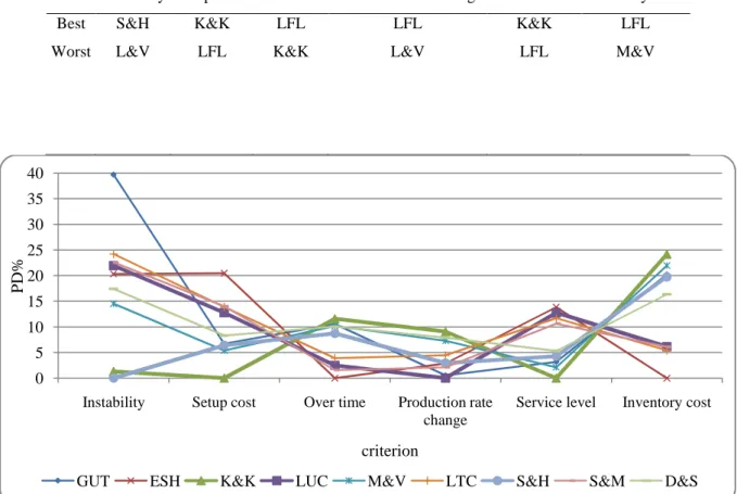
Table 4 shows the average amount of each criterion (Step 6)in 324 different cases for thirteen MPS development methods. Also, in each criterion, top 3 methods are specified by grey color. Table 5 shows the best and the worst MPS development methods if only a given criterion is important for decision making.
When decision maker is indifferent to the criteria, the following points might be resulted:
• Partly conflict between the criteria is obvious in Table 4.
Both row-by-row and column-by-column analyses are possible for Table 4. In a row-by row analysis, the best criterion performance of each method compared to the others is obtained. For example, the best performance of GUT compared to the others is in production rate change as well as service level, whereas that of ESH is in overtime and inventory cost.
• In a column-by-column analysis, the top 3 methods in a given criterion are obtained. According to Table 5, LFL has a fluctuating performance as it has the best performance in overtime, production rate change and inventory costs criteria while has the worst performance in setup costs and service level. In fact, its performance is an explicit function of criteria; it seems that we can say nothing about it without weighting the criteria.
Table 3. Different scenarios of data
Scenario values # of
scenarios Notation
Parameter
Low: 1.01 – High: 1.25 2
CT Capacity tightness
Uniform [1,2] 1
h Unit inventory cost
Low: Uniform[200,500] – High: Uniform[1000,4000] 2
SC setup costs
Low: Uniform[4,5] Medium: Uniform[10,12] – High: Uniform[24,30] – 3
B Unit shortage cost
Low:0.1 Medium:0.2 – High:0.4 – 3
DV Demand variation
Low:0.1 Medium:0.2 – High:0.4 – 3
MV Product mix variation
Low:0 Medium:0.05 – High:0.1 – 3
EB Forecast error
8 1
PH Planning horizon
0.25 1
FP Freezing proportion
1 1
RP Replanning Periodicity
• L&V method has the worst performance in two out of all criteria while is not among the top 3 performances in no other criterion. Accordingly, without weighting, it may be put aside.
• PPB and MOO methods are not among the top 3 performances; therefore, they are also not considered in the following analysis.
• For nine remaining methods, figure. 2 depicts the percent deviation from the best performance in each criterion (PD%) which is calculated by equation (5).
+&12% =45674567456 . 100 (5)
where Valmn and BValn are the performance of criterion n for method m and the best performance of criterion n, respectively.
• If the average PD% of the above nine methods are calculated, S&H, K&K and LUC methods have the lowest average percent deviation (7%, 8%, and 9%, respectively) from the best performance considering all the criteria with equal weights.
The criteria’s weights obtained from Shannon entropy are given in Table 6. Based on the results, inventory costs, setup costs and instability with the weights of 0.32, 0.26 and 0.24, respectively, have the highest importance among the criteria.
Using the TOPSIS method for Table4,the corresponding ranking of thirteen MPS development methods is shown in Figure.3.CL is the output of TOPSIS and indicates the relative closeness to each method of ideal solution.
• It is worth noting that LFL and ESH generate high setup costs and low service levels; however, because of the lowest inventory costs and instability (with top weights), they gain the first and second ranks.
• In contrast, GUT and L&V with high inventory and setup costs (with top weights) gain the two last places in the ranking.
In Table 8, the performance of each MPS development method will be discussed according to the implementation in 324 cases. We consider a good performance if TOPSIS rank is among the top 3 and poor performance if among the bottom 3.
3-3- Analyzing the effect of critical parameters
In this subsection, we discuss the effect of critical parameters on the performance of MPS development methods.
Table 4. Overall performance of MPS development methods before weighting criteria
Instability Setup costs Over time Production rate change Service level Inventory costs
GUT 43.3 67313 14187 27526 0.91 16707
ESH 37.3 75983 12829 28153 0.81 13896
K&K 31.4 63077 14314 29851 0.94 17252
L&V 43.9 67433 13591 30916 0.90 16543
LFL 31.1 99768 12380 26782 0.70 9843
LUC 37.8 71119 13149 27370 0.82 14747
M&V 35.5 66473 14135 29368 0.92 16947
LTC 38.5 71829 13328 28586 0.83 14648
S&H 31.0 67116 13947 28175 0.90 16642
S&M 38.0 71928 13031 27946 0.84 14743
D&S 36.4 68325 14123 29530 0.89 16171
PPB 40.3 70691 13198 27954 0.85 14946
MOO 33.2 69154 13323 30865 0.87 15893
Table 5. The best and worst MPS development methods in each criterion
Instability Setup costs Over time Production rate change Service level Inventory costs
Best S&H K&K LFL LFL K&K LFL
Worst L&V LFL K&K L&V LFL M&V
Fig. 2. Comparing PD% of MPS development methods before weighting criterion
0 5 10 15 20 25 30 35 40
Instability Setup cost Over time Production rate change
Service level Inventory cost
P
D
%
criterion
Table 6.
Fig.3.Overall
Table 7.
Method LFL ESH LUC K&K
Rank 1 2 3
- Capacity tightness
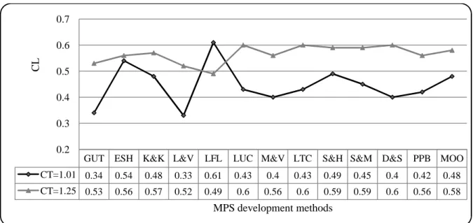
Notably, when capacity tightness is reduced (i.e., the available capacity is increased), the importance (weight) of customer service level is increased. Performance of MPS development methods under different capacity tightness is shown in
•When CT=1.01, based on the Shannon entropy
level with the weights of 0.29, 0.23, 0.19 and 0.13,respectively, have the highest priorities. CT=1.25, setup costs, inventory cost
respectively, have the highest importance
•In CT=1.25, as the more available are close.
•LFL, as the best method, in both scenarios (i.e., but high setup costs and low service level
•When CT=1.01, LFL and ESH have the first two ranks. However, if are as the best; in this scenario, LFL
•ESH and somewhat K&K and S&H are not sensitive to
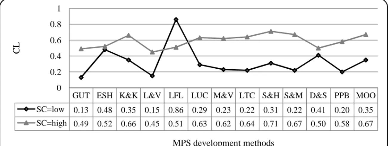
- Setup cost
Performance of MPS development methods versus unit
performances when SC is low and high are very different. LFL for both scenarios of inventory costs, overtime and service level (with high importance).
change and overtime are going to increase. 0.4
0.45 0.5 0.55 0.6
LFL ESH LUC
C
L
Criteria’s weight obtained from Shannon entropy. Rank Criterion Weight
1 Inventory costs 0.32 2 Setup costs 0.26 3 Instability 0.24 4 Service level 0.10 5 Production rate change 0.04
6 Over time 0.04
Overall performance of MPS development methods
Table 7.Rank of MPS development methods
K&K LTC S&H S&M MOO PPB D&S
4 5 6 7 8 9 10
Notably, when capacity tightness is reduced (i.e., the available capacity is increased), the importance (weight) of customer service level is increased. Performance of MPS development methods under different capacity tightness is shown in figure. 4. By increasing CT, instability is going to increase.
Shannon entropy, inventory costs, instability, setup c
level with the weights of 0.29, 0.23, 0.19 and 0.13,respectively, have the highest priorities. , inventory costs and instability with the weights of 0.31, 0.29 and 0.23,
importance.
available capacity and fewer shortages, service levels for different methods LFL, as the best method, in both scenarios (i.e., CT=1.01,1.25) has low inventory cost
and low service level.
=1.01, LFL and ESH have the first two ranks. However, if CT=1.25, D&S, LUC, and LTC are as the best; in this scenario, LFL has the worst performance.
ESH and somewhat K&K and S&H are not sensitive to CT parameter.
Performance of MPS development methods versus unit setup cost is shown in Fig. 5. T is low and high are very different. LFL for both scenarios of
, overtime and service level (with high importance). By increasing SC, production rate change and overtime are going to increase.
LUC K&K LTC S&H S&M MOO PPB D&S M&V
MPS development methods
M&V L&V GUT 11 12 13
Notably, when capacity tightness is reduced (i.e., the available capacity is increased), the importance (weight) of customer service level is increased. Performance of MPS development methods under
, instability is going to increase. , instability, setup costs, and service level with the weights of 0.29, 0.23, 0.19 and 0.13,respectively, have the highest priorities. When and instability with the weights of 0.31, 0.29 and 0.23, and fewer shortages, service levels for different methods =1.01,1.25) has low inventory costs and overtime, =1.25, D&S, LUC, and LTC
setup cost is shown in Fig. 5. The is low and high are very different. LFL for both scenarios of SC has the lowest y increasing SC, production rate
•In low SC, inventory costs and instability, whereas in high SC, instability, setup and inventory costs have the maximum weights.
•When SC is low, LFL and if SC is high, S&H is as the best. Notably, if SC is high, LFL is among the methods with poor performances.
•Though MPS development methods are very sensitive to SC, ESH and D&S are not sensitive.
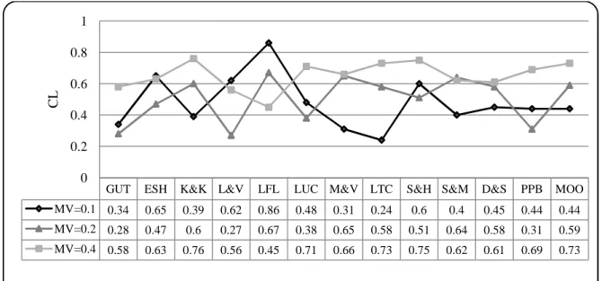
- Product mix variation
Figure 6 shows the performance of MPS development methods versus MV parameter. It is worth noting that in each three scenarios, the instability criterion has the highest weight. Also, the performances are very sensitive to the product mix variation.
•When MV is high, LFL is the worst method; but, in the other two scenarios (i.e. medium and low), it has the best performance.
•If MV is low, LFL and LTC are as the best and worst methods, respectively; when MV is medium, LFL and L&V have the best and worst performances; if MV is high; however, K&K and LFL are as the first and last rank methods. MOO gains a medium rank in all three scenarios of MV.
•The performance of LTC has a direct positive relation to MV so that it reaches from the last rank up to the third place by increasing DV. A somewhat similar trend is observed for K&K, M&V, D&S, and MOO. In contrast, LFL has a direct negative relation to MV, as its rank is weakened from the first down to the last by increasing DV.
•Though MPS development methods are very sensitive to MV, ESH is not so sensitive.
- Total demand variation
In figure 7, we depict the performance of MPS development methods versus DV parameter. Note worthily, with increasing DV, service level, overtime and setup costs of MPS development methods are majorly improved. Also, the performances are sensitive to demand variation.
•When DV is low or medium, LFL is best method; if it is high, it has also a good performance.
•If DV is low, LFL and K&K are as the best and worst methods, respectively; when DV is medium, LFL has the best performance while L&V, S&M, and D&S are of the worst performance; if DV is high; however, K&K and L&V are as the first and last rank methods. MOO gains a medium rank in all three scenarios of MV.
•The performance of K&K has a direct positive relation to DV so that it reaches from the last rank up in the first place by increasing DV. A somewhat similar trend is observed for S&H. In contrast, LFL and ESH have direct negative relations to DV, as their ranks are weakened by increasing DV.
Fig. 4.Performance of MPS development methods versus capacity tightness
GUT ESH K&K L&V LFL LUC M&V LTC S&H S&M D&S PPB MOO CT=1.01 0.34 0.54 0.48 0.33 0.61 0.43 0.4 0.43 0.49 0.45 0.4 0.42 0.48 CT=1.25 0.53 0.56 0.57 0.52 0.49 0.6 0.56 0.6 0.59 0.59 0.6 0.56 0.58
0.2 0.3 0.4 0.5 0.6 0.7
C
L
Fig. 5. Performance of MPS development methods versus setup costs
Table 8.Performance analysis of MPS development methods
Method Sensitivity Insensitivity
P
er
fo
rm
an
ce
Combination
(DV, MV, CT, EB, SC) Dominant characteristic
GUT DV SC Best (H
I
,-,H,LIII,-) High service level
Worth (L,-,L,-,MII,-) High instability and inventory costs
ESH DV,MV,SC - Best (M,L,L,-,L) Low instability and inventory costs
Worth (-,-,H,L,H) High instability and setup costs
K&K DV,MV,EB SC Best (-,H,-,L,-) Low instability and setup costs-high service level
Worth (L,L,-,-,-) High instability and inventory costs
L&V MV EB,SC,CT Best (-,L,H,M,-) Low instability and inventory costs
Worth (H,H/MIV,L,-,-) The highest instability
LFL SC,CT - Best (L,L,L,-,L) Low instability-lowest inventory costs
Worth (-,-,H,-,H) High setup costs-low service level
LTC DV SC,CT Best (L,H,H,M,-) Low instability and inventory costs
Worth (H,L,-,H,L) Low service level-high setup costs
LUC MV,CT SC Best (-,-,H,M,-) Low instability and inventory costs-high productionrate change
Worth (-,M,-,-,-) High overtime, setup costs and productionrate change
M&V MV,EB SC Best (-,M,-,H,-) Highest service level-low setup costs
Worth (-,L,L,L,-) High instability and production rate change
S&H DV,SC CT Best (H,H/L
V
,-,-,H) Low instability and inventory costs-high service level
Worth (L,L,-,M,-) High inventory costs
S&M SC EB,CT
Best (-,M,-,-,H) Low instability and production rate change
Worth (M,L,-,-,L)
(-,H/L,L,H,-) High setup costs-Low service level
D&S CT, SC EB Best (-,-,H,H,H) Low instability-high service level
Worth (M,H,L,-,-) High overtime and inventory costs
PPB EB,DV CT Best (M,-,-,L,H) Low instability, inventory costs, and production rate change
Worth (L,M,-,H,-) High instability and setup costs
MOO DV CT,SC Best
(M/LVI,-,-,M/L,H)
(-,H,-,-,H) Low instability and inventory costs-high service level
Worth (H,L,-,-,-) High instability, production rate change, and overtime
I High, II Medium, III Low, IV High or medium, V High or low, VI Medium or low
GUT ESH K&K L&V LFL LUC M&V LTC S&H S&M D&S PPB MOO SC=low 0.13 0.48 0.35 0.15 0.86 0.29 0.23 0.22 0.31 0.22 0.41 0.20 0.35 SC=high 0.49 0.52 0.66 0.45 0.51 0.63 0.62 0.64 0.71 0.67 0.50 0.58 0.67
0 0.2 0.4 0.6 0.8 1
C
L
Fig. 6. Performance of MPS development methods versos product mix variation.
•GUT, K&K, and S&H are more sensitive to DV than the other methods.
•Though MPS development methods are sensitive to DV, ESH and LFL are not so.
Fig.7. Performance of MPS development methods versus demand variation
- Forecast error
Figure 8 shows the performance of MPS development methods versus EB parameter. Notably, inventory costs, instability, and production rate change values of MPS development methods are improved when decreasing forecast error. By increasing EB, it tries to use capacity better in order to produce more items leading to increase in production costs and service level.
•When EB is low or medium, LFL is the best method with superior performance; but, if it is high, it has the worst performance.
GUT ESH K&K L&V LFL LUC M&V LTC S&H S&M D&S PPB MOO
MV=0.1 0.34 0.65 0.39 0.62 0.86 0.48 0.31 0.24 0.6 0.4 0.45 0.44 0.44
MV=0.2 0.28 0.47 0.6 0.27 0.67 0.38 0.65 0.58 0.51 0.64 0.58 0.31 0.59
MV=0.4 0.58 0.63 0.76 0.56 0.45 0.71 0.66 0.73 0.75 0.62 0.61 0.69 0.73
0 0.2 0.4 0.6 0.8 1
C
L
MPS development methods
GUT ESH K&K L&V LFL LUC M&V LTC S&H S&M D&S PPB MOO
DV=0.1 0.3 0.58 0.25 0.43 0.8 0.46 0.43 0.61 0.33 0.52 0.52 0.29 0.53
DV=0.2 0.36 0.53 0.5 0.29 0.71 0.39 0.3 0.35 0.5 0.29 0.29 0.53 0.52
DV=0.4 0.59 0.43 0.68 0.28 0.62 0.56 0.54 0.41 0.62 0.58 0.49 0.47 0.42
0.2 0.3 0.4 0.5 0.6 0.7 0.8 0.9
C
L
•If EB is low, LFL and M&V are as the best and worst methods, respectively; if EB is medium, LFL and GUT have the best and worst performances; when DV is high; however, K&K and LFL are as the first and last rank methods. MOO gains a medium rank in all three scenarios of MV.
•In medium EB, LFL and ESH have the lowest inventory costs. K&K and LFL have the highest and lowest service level, respectively. GUT and PPB have the highest instability. The greatest weight is given to instability and setup costs and caused that LFL and ESH have the highest scores.
•With high EB, over 80% of weight is for instability, setup and inventory cost.LFL and ESH have the lowest and GUT the highest inventory cost.
•L&V and M&V are the most sensitive to EV while PPB and MOO has the lowest sensitivity.
Fig 8. Performance of MPS development methods versus EB parameter
4- Implementation in Yazd Wire &Cable Company
In order to compare thirteen MPS development methods in practice using the proposed framework, we employ the data of Yazd Wire & Cable Company. It has six product groups; we study the control cable product groups. The group has seven products that everyone needs to have a main common resource; the product shares in the resource are 0.05, 0.04, 0.01, 0.28, 0.12, 0.02 and 0.03, respectively. Real demands for eight weeks are given in Table9. Available capacity is 3300 min; 2640 minas normal capacity. CT is equal to 1.06.
In general, we use Shannon entropy to weight the criteria. But, Yazd Wire & Cable company’s expert opinions are available; hence, we use fuzzy AHP instead of Shannon entropy for weighting the criteria. Fuzzy AHP allows decision makers to focus only on the paired comparisons of criteria and express their own preferences subjectively. In the existing conditions of company, CT is low and DV, MV, SC and EB are in high scenario. Fuzzy AHP questionnaire was given to 11 employees; the resulted weights are given in Table 10.
Table 9. Real demands in Yazd Wire & Cable Company
product week
1 2 3 4 5 6 7 8 1 306 280 572 268 1307 956 2435 2896 2 40 20 27 97 97 460 97 168 3 29 36 0 0 31 5 83 23 4 188 100 295 89 1210 953 762 462 5 27 57 183 41 524 342 398 169 6 20 23 74 10 0 398 125 648 7 110 10 12 0 57 118 140 259
GUT ESH K&K L&V LFL LUC M&V LTC S&H S&M D&S PPB MOO
EB=0 0.11 0.12 0.19 0.06 0.98 0.19 0.05 0.27 0.32 0.21 0.16 0.32 0.39
EB=0.5 0.3 0.53 0.35 0.33 0.67 0.51 0.33 0.53 0.33 0.44 0.33 0.37 0.45
EB=1 0.61 0.67 0.84 0.58 0.27 0.64 0.79 0.57 0.82 0.61 0.74 0.62 0.78
0 0.2 0.4 0.6 0.8 1
C
L
Table 10.Criteria’ weight in Yazd Wire & Cable Company
criterion Instability Setup cost weight 0.34 0.18
rank 1 2
Based on the results of Table 10
using the proposed framework are shown in low and DV, MV, SC and EB are high very good performances while LTC and Wire & Cable Company, confirms a
framework and results may direct similar companies to determine the best MPS development method.
Fig.9.Performance of MPS development methods in Yazd Wire & Cable Company
5- Concluding remarks
MPS may be considered as an NP
this study was to compare thirteen alternative MPS development method in multi-product single level production environment. An MCDM was proposed to compare and analyze
conditions. Shannon entropy was used to weight the criteria
alternatives. 324 different combinations by establishing multiple scenarios of operating parameters including capacity tightness, setup cost, forecast error, demand variation, product mix variation and shortage cost was considered and a comprehensive numerical simulatio
results of Shannon entropy, inventory cost
Although results show that the performance of MPS development m
weights as well as the operating conditions; but, in general, LFL and ESH are the best methods because they have low inventory costs and instability as
ESH and LFL has the low and high sensitivity to all the operating conditions, respectively. We also studied the performance of all the alternative metho
operating parameters. In order to implement in practice, we used the data of Yazd Wire & Cable Company to compare thirteen MPS development methods.
0.3 0.4 0.5 0.6 0.7 0.8
S&H MOO K&K
C
L
’ weight in Yazd Wire & Cable Company using fuzzy AHP Setup cost Service level Inventory cost Production rate change
18 0.17 0.12 0.11
3 4 5
Based on the results of Table 10, the corresponding priorities of thirteen MPS development methods are shown in figure. 9.In the previous section, we show that when are high (i.e., existing company condition), S&H, MOO and K&K have while LTC and L&V are of poor performances. Fig. 9, related to the Yazd Wire & Cable Company, confirms a consistency in the results. So, it seems that the proposed direct similar companies to determine the best MPS development method.
Performance of MPS development methods in Yazd Wire & Cable Company
sidered as an NP-hard capacity-constrained lot-sizing problem; therefore, the aim of this study was to compare thirteen alternative MPS development methods according to six main criteria
product single level production environment. An MCDM with numerical simulation
was proposed to compare and analyze the different MPS development methods under various operating opy was used to weight the criteria and TOPSIS was proposed to rank 324 different combinations by establishing multiple scenarios of operating parameters including capacity tightness, setup cost, forecast error, demand variation, product mix variation and shortage cost was considered and a comprehensive numerical simulation was directed. Based on the
, inventory costs, setup costs and instability have the highest Although results show that the performance of MPS development methods is a function of
weights as well as the operating conditions; but, in general, LFL and ESH are the best methods because they have low inventory costs and instability as the most important criteria. Significant characteristic of ESH and LFL has the low and high sensitivity to all the operating conditions, respectively. We also studied the performance of all the alternative methods in terms of both the criteria
operating parameters. In order to implement in practice, we used the data of Yazd Wire & Cable Company to compare thirteen MPS development methods.
K&K D&S M&V ESH GUT LFL PPB LUC L&V
MPS development methods
using fuzzy AHP
Production rate change Overtime 0.08
6
MPS development methods . 9.In the previous section, we show that when CT is , S&H, MOO and K&K have . Fig. 9, related to the Yazd the results. So, it seems that the proposed direct similar companies to determine the best MPS development method.
Performance of MPS development methods in Yazd Wire & Cable Company
sizing problem; therefore, the aim of s according to six main criteria numerical simulation framework different MPS development methods under various operating and TOPSIS was proposed to rank the 324 different combinations by establishing multiple scenarios of operating parameters including capacity tightness, setup cost, forecast error, demand variation, product mix variation and n was directed. Based on the and instability have the highest importance. ethods is a function of the criteria’ weights as well as the operating conditions; but, in general, LFL and ESH are the best methods because . Significant characteristic of ESH and LFL has the low and high sensitivity to all the operating conditions, respectively. We also s in terms of both the criteria as well as the operating parameters. In order to implement in practice, we used the data of Yazd Wire & Cable
References
Akhoondi, F., Lotfi, M.M.(2016). A heuristic algorithm for master production scheduling problem with controllable processing times and scenario-based demands, International Journal of Production Research, 54(12): 3659-3676.
Dixon, P.S., Silver, E.A.(1981). A heuristic solution procedure for the multi-item, single level, limited capacity, lot sizing problem, Journal of Operations Management, 2 (1): 23-40.
Eisenhut, P.S.(1975). A dynamic lot sizing algorithm with capacity constraints, IIE Transactions, 7 (2): 170-176.
Gahm, C., Dünnwald, B., Sahamie, R.(2014).A multi-criteria master production scheduling approach for special purpose machinery, International Journal of Production Economics,149: 89-101.
Gunther, H.O.(1987). Planning lot sizes and capacity requirements in a single stage production systems, European Journal of Operational Research, 31 (2): 223-231.
Hajipour, V., Fattahi, P., Nobari, A. (2014). A hybrid ant colony optimization algorithm to optimize capacitated lot-sizing problem, Journal of Industrial and Systems Engineering, 7(1):1-20.
Heemsbergen, B., Malstrom, E.M. (1994). A simulation of single-level MRP lot sizing heuristics: an analysis of performance by rule, Production Planning & Control, 5(4): 381-391.
Herrera, C., Belmokhtar-Berraf, S., Thomas, A., Parada, V.(2015). A reactive decision-making approach to reduce instability in a master production schedule, International Journal of Production Research, 54(8): 2394-2404.
Jeunet, J., Jonard, N.(2000). Measuring the performance of lot-sizing technique in uncertain environment, International Journal of Production Economics, 64 (1-3): 197-208.
Jonsson, P., Kjellsdotter, L.(2015).Improving performance with sophisticated master production scheduling, International Journal of Production Economics, 168, 118-130.
Karimi, B., Ghomi Fatemi, S.M.T., Wilson, J.M. (2003). The capacitated lot sizing problem: a review of models and algorithms, Omega, The international Journal of management science, 31: 365-378.
Kirca, O., Kokten, M.(1994). A new heuristic approach for the multi-item dynamic lot sizing problem, European Journal of Operational Research, 75 (2): 332-3241.
Lambrecht, M.R., Vanderveken, H.(1979).Heuristic procedures for the single operation, multi-item loading problem, IIE Transactions, 11 (4): 319-325.
Maes, J., Van Wassenhove, L.N.(1986). A simple heuristic for the multi-item single level capacitated lot sizing problem, Operations Research Letters, 4 (6): 265-273.
Ponsignon, T., Mönch, L.(2014). Simulation-based performance assessment of master planning approaches in semiconductor manufacturing, Omega, The international Journal of management science, 46: 21-35.
Razmi, J., Lotfi, M.M. (2011). Principles of production planning and inventory control, Tehran University Publications.
Selen, W.J., Heuts, R.M.(1989). A modified priority index for Gunther’s lot-sizing heuristic under capacitated single stage production, European Journal of Operational Research, 41 (2): 181-185.
Soares, M.M., Vieira, G.E.(2009).A new multi-objective optimization method for master production scheduling problems based on genetic algorithm, International Journal of Advanced Manufacturing Technology, 41 (5): 549-567.
Sridharan, S., Beny, W., Udaya Bhanu, V.(1988). Measuring master production schedule stability under rolling planning horizon, Decision Sciences, 19 (1): 147-166.
Supriyanto, I., Noche, B.(2011). Fuzzy multi-objective linear programming and simulation approach to the development of valid and realistic master production schedule, Logistics Journal, 7: 1-14. Unahabhokha, C., Schuster, E.W., Allen, S.J., Finch, B.J. (2003). Master production schedule stability under conditions of finite capacity, Working Paper, Massachusetts Instituteof Technology.
Vieira, G.E., Favaretto, F. (2006). A new and practical heuristic for master production scheduling creation, International Journal of ProductionResearch, 44(18-19): 3607-3625.
Xie, J., Zhao, X., Lee, T.S. (2003). Freezing the master production schedule under single resource constraint and demand uncertainty, International Journal of Production Economics, 83 (1): 65-84. Xie, J., Zhao, X., Lee, T.S.,Zhao, X. (2004). Impact of forecasting error on the performance of capacitatedmulti-item production systems, Computers & Industrial Engineering, 46 (2): 205-219. Zhao, X., Lam, K. (1997). Lot-sizing rules and freezing the master production schedule in material requirements planning system, International Journal of Production Economics, 53 (3): 281-305. Zhao, X., Xie, J. (1998). Multilevel lot-sizing heuristics and freezing themaster production schedule in material requirements planning systems, Production Planning & Control, 9(4): 371-384.
Zhao, X.,Xie, J., Jiang, G.S. (2001). Lot-sizing rule and freezing themaster production schedule undercapacity constraint and deterministic demand, Production and operations management, 10 (1): 45-67.
![Table 3. Different scenarios of data Scenario values # of scenarios Notation Parameter Low: 1.01 – High: 1.25 2 CT Capacity tightness Uniform [1,2] 1 h](https://thumb-us.123doks.com/thumbv2/123dok_us/8370898.2223223/9.892.90.807.131.446/different-scenarios-scenario-scenarios-notation-parameter-capacity-tightness.webp)