Sharif University of Technology
Scientia IranicaTransactions A: Civil Engineering http://scientiairanica.sharif.edu
Robust model and solution algorithm for the railroad
blocking problem under uncertainty
R. M. Hasany and Y. Shafahi
Department of Civil Engineering, Sharif University of Technology, Tehran, P.O. Box 11155-8639, Iran. Received 30 December 2015; received in revised form 21 December 2016; accepted 4 March 2017
KEYWORDS Railroad blocking problem;
Robust optimization; Branch-and-cut algorithm; Uncertainty; Railway planning.
Abstract. The railroad blocking problem emerges as an important issue at the tactical level of planning in freight rail transportation. This problem consists of determining the optimal paths for freight cars in a rail network. Often, demand and supply resource indicators are assumed certain; hence, the solution obtained from a certain model might not be optimal or even feasible in practice due to the stochastic nature of these parameters. To address this issue, this paper develops a robust model for this problem with uncertain demand and travel time as supply resource indicators. Since the model combines integer variables and nonlinear functions, a branch-and-cut algorithm is used to solve the linearized version of the robust model. The performance of the proposed algorithm in several instances is examined and discussed. The high eciency and eectiveness of the proposed algorithm are demonstrated through a comparison with a well-known solver. Finally, this algorithm is applied to a blocking problem of the railways of Iran. The results show that, by ignoring approximately 10% of the optimal value of the deterministic model, we have an optimal solution that remains unchanged with a probability of more than 0.98.
© 2018 Sharif University of Technology. All rights reserved.
1. Introduction
1.1. Railroad blocking problem
The planning problems in railway transportation are classied into strategic, tactical, and operational lev-els [1,2]. The strategic level is concerned with long-term planning that requires a large amount of invest-ment. High-level managers who design and execute strategic decisions to paint a picture of the long-term goals of the railway system make the decisions at this level. The tactical level supports the strategic level by translating strategic decisions into specic decisions relevant to a distinct area of railway planning. Indeed,
*. Corresponding author. Tel.: +98 21 66164246; Fax: +98 21 66014828
E-mail addresses: [email protected] (R. M. Hasany); [email protected] (Y. Shafahi)
doi: 10.24200/sci.2017.4199
the tactical level is the connection between the strategic and operational levels. The operational level lies at the bottom of railway planning. The decisions at this level are focused on specic procedures and are made by frontline managers.
Finding the optimal paths for freight cars, i.e., the so-called blocking problem, is an important issue at the tactical planning level [3]. There are three approaches to sending each shipment (i.e., the number of cars with the same origin-destination pair) through a rail network. In the rst approach, the cars that are associated with a shipment are assigned to the path with the least travel time, which sends them by a direct train that does not stop at any classication yard (which is the station with the ability to separate, sort, and assemble trains) until reaching its destination. If the number of cars associated with a shipment is approximately equal to the train's hauling capacity, the rst approach can be reasonable; however, the number of cars associated with a shipment is usually less than
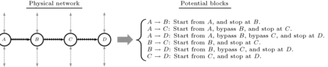
Figure 1. Potential blocks in a small example.
the hauling capacity of the outgoing train [4], and using this approach will lead to dispatching trains at their under-hauling capacities. The second approach focuses on dispatching trains at their near-hauling capacities by assembling the incoming cars in a classication yard as long as the number of cars does not exceed the hauling capacity of the train. Because the cars are not grouped at their origins based on their destinations, the cars can stop at several classication yards on the way to their destinations, causing delay in shipments. For instance, Barnhart et al. [5] reported that stopping at each classication yard would lead to a one-day delay; further, Bontekoning and Priemus [6] reported that classication operations could take 10 to 50% of train travel time. The third approach adopts the optimization techniques allowing a train to enter into some, but not all, classication yards to improve the performance of the rail system. In particular, this approach involves identifying the list of visited classication yards for each shipment to minimize the objective function (such as moving time and delay time experienced inside the yards) while satisfying railway restrictions. Note that the third approach can be stated as the general form, and the two earlier approaches are only special, extreme cases of the general form. The railroad blocking problem focuses on solving the general form to obtain the optimal path for each shipment.
Four important terms with respect to the railroad blocking problem should be dened. First, a block, consisting of a sequence of physical links, is a key element in the railroad blocking problem. If the cars are traveling across a block, they are not classied as long as they reach the end of that block. Every block is associated with two nodes: the start node, where the cars are attached to the departing train; and the end node, where the cars are released from the train. Second, the blocking network consists of a set of blocks and their corresponding nodes that are origin, destination, or classication yards. Third, the blocking path of a shipment is dened as a sequence of blocks that connects the origin to the destination for that shipment. Fourth, a feasible solution to the blocking problem is called the blocking plan, consisting of a set of blocking paths for all shipments.
To clarify the denitions, consider a small rail (physical) network with four nodes connected by three
arcs, which can be a part of a large network. Let nodes A and B be the origins and nodes C and D be the destinations. The four shipments are shipment 1 (from A to C), shipment 2 (from A to D), shipment 3 (from B to C), and shipment 4 (from B to D). Nodes B and C operate as classication yards in this network. The network and the list of potential blocks are shown in Figure 1. As an example, consider block A!D. Through this block, a train starts moving from node A, bypasses nodes B and C, and nally stops at node D. The potential blocks create four blocking plans, as shown in Table 1. Consider blocking plan 4 with three blocks. Shipments 1 and 2 move through block A!C. At node C, shipment 1 reaches its destination, while shipment 2 is released from the train at node C. Shipments 3 and 4 move through block B!C, and shipment 3 reaches its destination at node C, while shipment 4 is released from the train at node C. Finally, shipments 2 and 4 move together through block C!D to reach their destination (node D).
1.2. Literature review of the railroad blocking problem
Several studies have examined the railroad blocking problem. Assad [3] initially introduced an integer linear program model for this problem. The objective functions of the model included the train costs (op-erating and delay costs through the rail tracks) and yard costs (classication and delay costs inside yards). The model included two constraints: each shipment is shipped from its origin to its destination, and the amount of ow moving through each block is bounded by block capacity. In addition to the Assad's objective function, other functions have been used frequently in the literature. Bodin et al. [7] derived a delay function in terms of car ow, which is added to train costs. Marin and Salmeron [8] considered investment to purchase new eets, in addition to the train costs. The number of visited classication yards was introduced by Fugenschuh et al. [4] as a crucial component of objective function.
Many realistic limitations were not presented in Assad's work. Eorts to consider more limitations have been undertaken, including a maximum limit on the number of cars that can be classied inside the yards [9], a maximum limit on the number of cars that can move through each block [10], a maximum limit
Table 1. An illustration of blocking plans.
No. Blocking plan Blocks Shipments Blocking paths
1
A ! B B ! C C ! D
1 A ! B ! C
2 A ! B ! C ! D
3 B ! C
4 B ! C ! D
2
A ! C A ! D B ! C B ! D
1 A ! C
2 A ! D
3 B ! C
4 B ! D
3
A ! B B ! C B ! D
1 A ! B ! C
2 A ! B ! D
3 B ! C
4 B ! D
4
A ! C B ! C C ! D
1 A ! C
2 A ! C ! D
3 B ! C
4 B ! C !D
on the sum of the blocks that leave the yards [11], a maximum limit on the time spent reaching the destination for each origin-destination pair [12], and the number of blocking paths with a positive ow for each shipment could be more than one path [13].
Solution algorithms for the railroad blocking problem can be categorized in two ways. One way is to design a metaheuristic that possibly achieves a good solution to the problem with a short running time. Re-searchers have made great eorts to design metaheuris-tics for the railroad blocking problem. Some examples include neural networks [14], genetic algorithms [15], simulated annealing [9], ant colony optimization [16], taboo searches [17], and local searches for three major United States' railroads [18]. Metaheuristics iteratively search among the feasible regions to nd the near-optimal solution with less computation time, compared to the exact algorithms for integer programming. How-ever, metaheuristics might not converge to the optimal solution, and this aw points to exact algorithms whose convergence to optimality is assured, which is categorized as the second way.
Bodin et al. started using exact algorithms for nding the optimal solution to the railroad blocking problem [7], and implemented a branch-and-bound algorithm using data from Norfolk and Western Rail-road. The branch-and-price algorithm was applied to the railroad blocking problem for a major domestic railroad in the United States [10], the Deutsche Bahn railroad [19], and some hypothetical networks [20]. Keaton [11] initially adopted the Lagrangian relaxation
method to decompose the original problem into two independent sub-problems for a portion of the Conrail system in the United States. Barnhart et al. [5] also adopted the Lagrangian relaxation method and added inequalities to the relaxed Lagrangian problem to lift the lower bounds. They used this algorithm for realistic network data provided by CSX transportation. Fugenschuh et al. [4] presented a mixed-integer, non-linear program and described two exact techniques and one heuristic to improve the proposed formulation.
There has been much attention paid to the impact of uncertainty on the results of railway planning [21-24]. Nevertheless, the blocking problem under uncertainty has been ignored. The study of Jin [25] is currently the only one available in the literature addressing this problem. In this study, the author introduced uncertainty in the nature of a demand and supply resource indicator in a limited number of scenarios to solve the uncertain model. Indeed, if the assumed values of random parameters are not equal to their values after realization, then the optimal solution might not be optimal or even feasible anymore [26].
1.3. Uncertainty in the railroad blocking problem
At the tactical level of railroad planning, the quantity of input parameters is often assumed certain and known. While the time horizon of tactical plan-ning varies from one to three months, disregarding uncertainty leads to a clear dierence between the optimal solutions of the deterministic and stochastic
models [27]. In the deterministic model, the nominal quantity of uncertain parameters can be calculated using dierent methods [28-30]; however, it has been reported that the nominal quantity of demand is over-or under-estimated [31], and the whole system could face an enormous amount of unexpected costs [32]. Additionally, the travel time spent through the rail network is severely aected by such factors as changing weather, eet availability, passing or overtaking, and moving of trains with higher priority (such as passenger trains) on the same track [6]. Thus, considering the demand and travel time as random parameters is much closer to reality.
Sensitivity analysis is a common tool used to address uncertainty in mathematical modeling. This method analyzes the optimal solution by changing the parameter values in a predened range. More precisely, it is necessary initially to solve the model with nominal data; then, by changing only one parameter within its range, it is necessary to ascertain whether the optimal solution remains optimal or not. Sensitivity analysis is assumed as the post-analysis method which only enables us to verify possible changes to the optimal solution as an input [33].
Stochastic programming is another tool that pro-vides a solution and takes advantage of probability distributions governing the data being known or able to be estimated. This approach has two main issues. First, the formulation of stochastic programming as-sumes that each uncertain parameter can be modeled as a random value with a valid probability distribution; therefore, this approach cannot be eective when the history data for the random parameter are not suf-cient. The second issue relates to the diculty of solving stochastic programming models, particularly in the presence of integer variables and nonlinear functions in the objective function or constraints.
Robust optimization is another approach to ad-dressing uncertainty in operations research, which is the focus of this paper. Several researchers have emphasized the subject of robust optimization. Soys-ter [34] modeled the robust counSoys-terpart of a linear program. The proposed model was very conservative, indicating that the dierence between the optimum val-ues for a deterministic model and its robust counterpart is considerably high. In light of this issue, Ben-Tal and Nemirovski [35] proposed a robust model for a linear program with uncertainty, which is inherent to technological coecients. The authors showed that the new robust model is less conservative than the model proposed by Soyster; in addition, the proposed model allowed for the control of the degree of conservatism.
In general, the robust approach has three advan-tages. Most importantly, the robust approach guar-antees the protection of the obtained solution against constraint violations due to the uncertainty parameter.
Since the blocking parameters usually change from month to month, the deterministic blocking plan must be subsequently re-optimized to obtain a new blocking plan for new realizations of uncertain parameters. If the new blocking plan is dierent from the previous blocking plan, then the train schedule required to carry a new set of blocks could be dierent from the previous schedule, and the previous locomotive and crew assignments might no longer be valid [36]. Second, the application of the robust approach will result in a model that requires less eort to solve, compared to the stochastic model. Third, the robust approach only requires a range of the uncertain parameters, rather than having a probability function for each uncertain parameter. It was reported that, for a stochastic parameter, the range is estimated much easier than probability function [37].
Our contributions made to the literature are mainly in two aspects: modeling and oering a solution algorithm. The rst contribution of this paper is that it proposes a robust blocking problem with uncertain demands and travel time as the supply resource indi-cators to produce a solution that is immunized against any realization of uncertain parameters in the ranges. The resulting model combines the diculty of discrete variables with the challenge of nonlinear functions in constraints. It is necessary to solve this model for realistic networks; however, the current state-of-the-art software is not able to nd the optimal solution or even produce a feasible solution in a reasonable amount of time. Therefore, the second contribution is devoted to the development of a specialized branch-and-cut algorithm. This algorithm involves running a branch-and-bound algorithm and using the process to generate a cut that is obtained by the linear approximation of the nonlinear terms in constraints.
The rest of the paper is organized as follows. Section 2 introduces the deterministic form of the blocking problem. Section 3 presents dierent sources of uncertainty in the blocking problem and the robust formulation of the deterministic model. Section 4 de-scribes a branch-and-cut method for solving the robust formulation of blocking problem. Section 5 shows numerical examples and a case study. Finally, Section 6 presents the main conclusions of the presented work. 2. Deterministic model for the blocking
problem
To explain uncertain parameters to the railroad block-ing problem, the presentation of the deterministic model is required. The model proposed by Newton et al. [10], which is one of the most commonly used models in the railroad blocking problem with certain parameters, is used in this section. The model is as follows:
Input parameters:
A The set of blocks indexed by a, K The set of shipments indexed by k, S The set of stations indexed by i, Qk The set of candidate blocking paths for
shipment k 2 K indexed by q, wai Time for separating and sorting each
car inside station i 2 S (hr), ta Traveling time for block a 2 A (hr),
a
q 1 if block a 2 A is on blocking path
q 2 Qk and 0 otherwise,
a
i 1 if station i 2 S is the start station of
block a 2 A and 0 otherwise, dk Demand value for shipment k 2 K
during the planning horizon (car), k
q Travel time of path q 2 Qk
for shipment k 2 K, that is, P
a2A(ta+
P
i2Siawai)aq (hr),
Vi The outow car capacity of station
i 2 S (car),
Wi The maximum number of blocks
directed out of station i 2 S,
ua The upper limit on car ows in block
a 2 A (car). Decision variables:
za : 1 if candidate block a 2 A is selected
and 0 otherwise, vk
q : Car ows associated with blocking
path q 2 Qk for k 2 K (car).
Barnhart et al. [5] presented the blocking problem as follows:
(P ) min
vk q;za
X
k2K
X
q2Qk k
qvqk; (1)
s.t. X
k2K
X
q2Qk a
qvkq uaza; 8 a 2 A; (2)
X
q2Qk vk
q dk; 8 k 2 K; (3)
X
a2A
a
iza Wi; 8 i 2 S; (4)
X
a2A
X
k2K
X
q2Qk a
qiavqk Vi; 8 i 2 S; (5)
vk
q 0; za 2 f0; 1g; 8 k 2 K;
8 q 2 Qk; 8 a 2 A: (6)
The objective function (1) minimizes the total travel time for shipments owing across the rail network. Constraint (2) limits the sum of ows between many origins to many destinations through block a 2 A to ua. Additionally, this constraint ensures that if
za = 0, then the blocking path q 2 Qk containing
block a 2 A, i.e., a
q = 1, is not involved in the solution.
Constraint (3) conserves the car ows of each shipment. Constraint (4) enforces the number of blocks directed out of any station to limit its block capacity. Similarly, Constraint (5) enforces the car ow directed out of any station to limit its volume capacity.
Above, Barnhart et al. [5] assumed that demand value and travel time are certain. In the rest of the paper, we present the robust formulation of the railroad blocking problem when these two parameters are uncertain.
3. Robust formulation of the railroad blocking problem
The aim of this section is to determine the optimal blocking paths for each shipment in the presence of uncertainty in demand value and travel time. Suppose that demand value, ~dk, and travel time, ~k
q, are
uncertain and belong to two bounded sets, Udk, and Uk
q. The denition of these two sets can be written as follows:
Udk = n
dk+ ^dk 1 1o; (7)
Uk q =
k
q + ^qk 1 1 : (8)
Let dk and k
q be the nominal values of demand
and travel time, respectively, and ^dk and ^k
q be the
maximum variations of demand value and travel time. The uncertain model for the blocking problem is given by the following:
(RP 1) min
vk q;za
X
k2K
X
q2Qk ~k
qvqk; (9)
s.t. X
q2Qk vk
q ~dk 8 k 2 K; (10)
Eqs. (2) and (4)-(6).
To develop the robust formulation of (RP 1), the methodology initially proposed by Ben-Tal and Nemirovski [26] is adopted. Note that these researchers only addressed uncertainty in the standard form, in which the technological coecients are the only source of uncertainty; however, the uncertain parameters in the blocking problem (i.e., ~dk and ~k
q) appear in
Constraint (10). To rewrite (RP 1) in the standard format, two modications are required [38]. The rst modication adds the objective function to the constraint set. To do so, an unrestricted decision variable, , which is equal to and greater than the objective function (9) is introduced; then, this con-straint is added to the concon-straint set. The second modication changes the role of the demand value in the technological coecient in Constraint (10). To do so, a variable, pk, is introduced for each k 2 K,
and ~dk appears as a coecient of pk provided that
pk = 1 always to obtain ~dkpk = ~dk. Using these two
modications, model (RP 1) can be rewritten in the standard format as follows:
(RP 2) min
vk q;za; ;pk
; (11)
s.t.
+X
k2K
X
q2Qk ~k
qvkq 0; (12)
X
q2Qk vk
q + ~dkpk 0 8 k 2 K; (13)
is free; pk = 1 8 k 2 K; (14)
Eqs. (2) and (4)-(6).
Based on the work of Ben-Tal and Ne-mirovski [26], the robust formulation of model (RP 2) is derived as follows. For further details on the conversion of (RP 2) to (RP 3) see the appendix.
(RP 3) min
vk
q;yqk;xkq;pk;sk;rk; ;za
; (15)
s.t.
+X
k2K
X
q2Qk k
qvkq +
X
k2K
X
q2Qk ^k
qykq
+ sX
k2K
X
q2Qk ^k
qxkq
2 0; (16)
yk
q vkq xkq yqk 8 k 2 K; 8 q 2 Qk;
(17) X
q2Qk vk
q + dkpk+ ^dksk+ k
r ^
dkrk2 0
8 k 2 K; (18)
sk pk rk sk 8 k 2 K; (19)
yk
q 0; sk 0 8 k 2 K; 8 q 2 Qk;
Eqs. (2), (4)-(6), and (14).
It has been shown that the optimal solution of (RP 3) will satisfy Constraints (12) and (13) with probability 1 exp( 2=2) and 1 exp( ( k)2=2),
respectively, where 0 and k 0 [26].
To simplify model (RP 3), the substitution of pk =
1 for all k 2 K into Constraints (18) and (19) yields the following constraints:
X
q2Qk vk
q + dk+ ^dksk+ kd^krk 0; 8 k 2 K;
(20)
sk 1 rk sk; 8 k 2 K: (21)
The term jrkj introduces non-linearity to
Con-straint (20). Two continuous variables (k
1and k2) and
one binary variable (k
3) are introduced for each k 2 K;
then, rk and jrkj are replaced by k
1 k2 and k1+ k2
in model (RP 3) [39]. To show the relationship among k
1, k2, and k3, the following logical constraints must
be considered, where M is an arbitrary, large value: k
1 Mk3 0; (22)
k
2 M 1 k3
0: (23)
Thus, nally, the robust counterpart of model (P ), denoted by (RP 4), is formulated as follows:
(RP 4) min
vk
q;yqk;xkq;pk;sk;k1;k2;k3; ;za
; (24)
s.t. X
q2Qk vk
q + dk+ ^dksk+ kd^k k1+ k2
0
8 k 2 K; (25)
sk 1 k
1 k2
sk; 8 k 2 K; (26)
k
1; k2 0; k3 2 f0; 1g ; 8 k 2 K; (27)
Eqs. (2), (4)-(6), (16), (17), (22), and (23).
After discarding the nonlinearity of Con-straint (18), model (RP 4) is an integer program with only one non-linear constraint, i.e., Constraint (16). However, this problem remains dicult to solve, even for small-sized problems; thus, an eective solution algorithm is required. The next section is devoted to development of the algorithm.
4. Solution algorithm
This section develops a specialized branch-and-cut algorithm, that is, a branch-and-bound algorithm is integrated into cut generation to solve the relaxation
of model (RP 4) at various branches of the branch-and-bound tree. To solve the model (RP 4), Constraint (16) is removed from model (RP 4), leaving only one integer linear program that possibly leads to a solution that violates Constraint (16). This violation can be managed by deriving a cut to remove the violated solution from the current feasible region.
The main component of the proposed algorithm approximates the nonlinear terms involved in Con-straint (16). If f( ; vk
q; yqk; xkq) is equal to:
+X
k2K
X
q2Qk k
qvqk+
X
k2K
X
q2Qk ^k
qykq
+ sX
k2K
X
q2Qk (^k
qxkq)2;
then the linear approximation of this function for variables ( ; vk
q; yqk; xkq) about ( ; vkq; ykq; xkq), using the
linear part of the Taylor series, is given by: f ; vk
q; yqk; xkqat ( ; vk
q; ykq; xkq) f ; v
k q; ykq; xkq
+ @f @ +X k2K X q2Qk @f @vk q vk
q vkq
+X k2K X q2Qk @f @yk q yk
q ykq
+X k2K X q2Qk @f @xk q (xk
q xkq): (28)
The derivatives of f(:) with respect to , vk q,
yk
q, and xkq are (-1), (qk), (^qk), and ^qk2xkq=
qP
k2K
P
q2Qk(^qkxkq)2, respectively; therefore, Ex-pression (28) can be rewritten as follows:
f ; vk
q; yqk; xkqat ( ; vk q; ykq; xkq)
+X
k2K
X
q2Qk k
qvqk+
X
k2K
X
q2Qk ^k
qyqk
+ X
k2K
X
q2Qk
^k2 q xkq
r P
k2K
P
q2Qk ^
k qxkq
2xkq
+ sX
k2K
X
q2Qk ^k
qxkq
2 X k2K X q2Qk ^k2 q xk2q
r P
k2K
P
q2Qk ^
k qxkq
2
: (29)
Suppose that ( ; vk
q; yqk; xkq; za; sk; k1; k2; k3) is the
op-timal value of variables ( ; vk
q; yqk; xkq; za; sk; k1; k2; k3)
in the relaxation of (RP 4). If this solution meets the integrality of za and k
3 and yet violates Constraint
(16), the following cut, (Relation (30)), is added to the list of constraints to cut o this solution in the remainder of the process:
f ; vk
q; yqk; xkqat ( ; vk
q; ykq; xkq) 0: (30) In the following, the detailed process of the proposed branch-and-cut algorithm is displayed to solve model (RP 4):
Step 0 (Initialization): Set ub = +1, lb = 1 and initialize the input parameters;
Step 1 (Termination test): If the termination condition is met, then the current solution is optimal; hence, go to Step 6;
Step 2 (Branch selection): If (i.e., a list of active branches) is empty, then it indicates that all of the possible branches have been investigated, so go to Step 6; otherwise, choose branch i 2 using the best-rst-search strategy;
Step 3 (Relaxation problem): Solve the re-laxation of model (RP 4) (which is model (RP 4) without Constraint (16) and without integrality constraints for za and k
3) for branch i. Let
( ; vk
q; yqk; xkq; za; sk; k1; k2; k3) be the optimal
solu-tion and set lb = max(lb; );
Step 4 (Cut generation): If (za; k
3) is not the
integer solution, then go to Step 3. If the value of:
+X
k2K
X
q2Qk k
qvkq +
X
k2K
X
q2Qk ^k
q ykq
+ sX
k2K
X
q2Qk (^k
qxkq)2
is strictly greater than zero, then add cut (30) to branch i, + branch i, and go to Step 1. Otherwise (i.e., + Pk2KPq2Qkqkvkq + P
k2K
P
q2Qk^qkyqk+ qP
k2K
P
q2Qk(^qkxkq)2 0), set:
ub = min(ub;X
k2K
X
q2Qk k
qvkq +
X
k2K
X
q2Qk ^k
q ykq
+ sX
k2K
X
q2Qk (^k
qxkq)2);
Step 5 (Branching): Branch on an integer variable with a fractional value in the optimal solution in Step 3, add two branches to set , and then go to Step 1;
Step 6 (Exit): End and report the optimal solution. The algorithm begins at Step 0 by determining the initial value for lb and ub, and inputting the data into the blocking network. The sets of blocks (A) and blocking paths (Qk) for each shipment k 2 K are
among the input sets. The set of blocks is chosen from all of the possible blocks being made from each origin to each yard, from each origin to each destination, from each yard to each destination, and from each yard to another yard. There exist many blocking paths for each shipment in the blocking network. The candidate set of blocking paths can be chosen in dierent fashions. One way is to use expert judgment to choose reasonable blocking paths. The other way is to use the k-shortest path algorithm and, then, choose the blocking paths with travel times that are less than the shortest travel time multiplied by a factor for each shipment. Barnhart et al. [5] suggested that this factor is equal to 1.5 to remove very long paths from the candidate set of blocking paths, assuming that no blocking path potentially in the optimal solution is ignored.
In Step 1, two termination conditions are dened, and the algorithm terminates as long as one condition is met. These conditions are: the relative gap (i.e., (ub lb)=ub) is less than "r; the absolute gap (i.e.,
ub lb) is less than "a.
Step 2 is dedicated to choosing a branch from set . Two classical branch selection strategies are the depth-rst-search and the best-rst-search. The former selects the deepest branch of the tree, and the latter follows the opposite strategy by choosing the un-explored branches with the smallest lower bound [40]. In this paper, the best-rst-search is used, which is the default setting of CPLEX [41]. Step 3 computes the solution of model (RP 4) without Constraint (16) and without integrality constraints for za and k
3 (called
relaxed model), and it obtains the optimal solution ( ; vk
q; yqk; xkq; za; sk; k1; k2; k3). In Step 4, a feasible
solution to (RP 4) is found provided that integer-feasible solution for za and k
3 is identied and it
does not violate Constraint (16). Otherwise, the linear approximation of this constraint (or cut (30)) is added to the tree to cut o the current solution from the potential solutions. Step 5 performs the process of splitting the integer variable, which is not integer feasible, into two branches. For example, consider the solution for a branch with za= 0:4. Two branches are
created from this branch: The rst branch is associated with za = 0, and the second branch is associated with
za = 1. Finally, Step 6 reports the optimal solution
obtained from the procedure.
5. Computational results
This section reports the computational results of the robust formulation of the railroad blocking problem under uncertainty in demand value and travel time for a number of hypothetical instances as well as the Iranian rail network. The proposed algorithm was coded in Vi-sual Basic and compiled with Microsoft ViVi-sual Studio, version 2010 using CPLEX software, version 12.2, with default settings and callback features. The experiments were performed on a Dell Latitude computer featuring a 2.66 Intel processor with 4 GB of RAM running Windows 7, X32 edition. To test the eciency of the proposed algorithm, the result of the algorithm was compared with the optimal solution found by GAMS 23.5 for model (RP 4) with the COUENNE solver. All tests were run within a one-hour time limit, and "rand
"a were assumed to be 1e-4 and 1e-5, respectively.
5.1. Test instances
Our tests were performed on 14 instances to study the eciency of the proposed algorithm. The instances are labeled with (A; B; C), where A, B, and C are the number of origins, classication yards, and desti-nations, respectively. Each instance is generated inside an (A 1) 100km (A 1) 100km region. Origin
a(= 1; ; A), classication yard b(= 1; ; B), and destination c(= 1; ; C) are located at coordinates (0; 100 (a 1)), (50 (A 1); 100A 1
B 1 (b 1)),
and (50 (A 1); 100A 1
C 1 (c 1)), respectively. The
generic region is illustrated in Figure 2.
It is necessary to limit the number of blocking paths for each shipment to ensure that GAMS does not terminate due to out-of-memory error. Herein, we assume that all blocking paths, which contribute to achievement of the optimal solution, are in the candidate set of blocking paths; therefore, in this paper, the blocking paths are considered for each shipment whose travel time is less than the shortest travel time multiplied by 3 (instead of 1.5 reported by Barnhart et al. [5]).
5.2. Evaluation of the proposed algorithm Fourteen dierent instances from (2,2,2) to (20,20,20) were considered; = 0:1, k = 0:1 for all k 2 K were
assumed. The demand ( ~dk) ranges were [dk d^k; dk+
^
dk], where dk = 1000 and ^dk = 200 for all k 2 K; the
travel time (~k
q) ranges were [qk ^qk; qk+ ^qk], where
k
q is calculated based on the average train speed being
equal to 60 km/h, and the value of ^k
q was set as a
random value between 0:1 k
q to 0:2 qk. Table 2
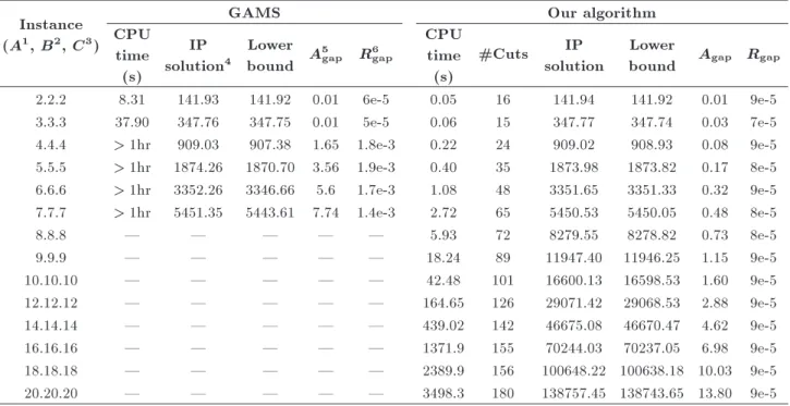
shows the test results for 14 instances and compares the eectiveness of the proposed algorithm and GAMS. This table shows that the proposed algorithm outperforms the GAMS results, and the algorithm is able to solve the instances optimally within one hour.
Figure 2. A scheme of the instances (A; B, C). Table 2. Computational results of 14 test instances. Instance
(A1, B2, C3)
GAMS Our algorithm
CPU time (s)
IP solution4
Lower bound A
5
gap R6gap
CPU time (s)
#Cuts IP
solution
Lower
bound Agap Rgap 2.2.2 8.31 141.93 141.92 0.01 6e-5 0.05 16 141.94 141.92 0.01 9e-5 3.3.3 37.90 347.76 347.75 0.01 5e-5 0.06 15 347.77 347.74 0.03 7e-5 4.4.4 > 1hr 909.03 907.38 1.65 1.8e-3 0.22 24 909.02 908.93 0.08 9e-5 5.5.5 > 1hr 1874.26 1870.70 3.56 1.9e-3 0.40 35 1873.98 1873.82 0.17 8e-5 6.6.6 > 1hr 3352.26 3346.66 5.6 1.7e-3 1.08 48 3351.65 3351.33 0.32 9e-5 7.7.7 > 1hr 5451.35 5443.61 7.74 1.4e-3 2.72 65 5450.53 5450.05 0.48 8e-5
8.8.8 | | | | | 5.93 72 8279.55 8278.82 0.73 8e-5
9.9.9 | | | | | 18.24 89 11947.40 11946.25 1.15 9e-5
10.10.10 | | | | | 42.48 101 16600.13 16598.53 1.60 9e-5
12.12.12 | | | | | 164.65 126 29071.42 29068.53 2.88 9e-5
14.14.14 | | | | | 439.02 142 46675.08 46670.47 4.62 9e-5
16.16.16 | | | | | 1371.9 155 70244.03 70237.05 6.98 9e-5
18.18.18 | | | | | 2389.9 156 100648.22 100638.18 10.03 9e-5
20.20.20 | | | | | 3498.3 180 138757.45 138743.65 13.80 9e-5
1. Number of origins; 2. Number of classication yards; 3. Number of destinations;
4. IP optimal value of the objective function in the unit of car-hr; 5. Absolute gap; 6. Relative gap.
However, GAMS could only solve 2 of the 14 instances optimally within one hour. Moreover, it is notable that this software was not even able to nd a feasible solution for 8 of the 14 instances.
Figure 3 shows the optimal values of ow variables for the deterministic and robust models in instance (5,5,5). In this gure, when moving away from the
cen-ter of the circle, the value of the ow variable increases on the logarithmic scale. It can be observed that the deterministic model addresses fewer paths with more ow value, whereas the robust model addresses more paths with less ow value. Specically, there are 25 paths (a single path for each of 25 shipments) with positive ow and the remainder of the paths with zero
Figure 3. Illustration of number of paths for
deterministic and robust optimal solutions for instance (5,5,5).
Figure 4. The value of the lower and upper bounds versus the number of cuts for instance (5,5,5).
values, overlapping in the center of the circle. However, the robust solution contains 66 paths with positive values, and each shipment is shipped with more than one path.
Figure 4 plots the value of the lower bound and upper bound versus the number of cuts, for instance, (5,5,5) in Step 4. As expected, the gap decreases as cuts are added.
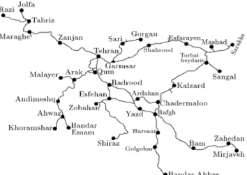
5.3. A case-study: Iran rail network
The real data were provided by studying railways in Iran to illustrate the application of the proposed algorithm to the blocking problem under demand and travel time uncertainty. The Iran rail network, which is approximately 12000 km length, has 334 stations, 44 classication yards, 1883 shipments, and 5058 blocks.
Figure 5. The abstract form of Iran rail network.
An abstract illustration of the Iranian rail network is provided in Figure 5.
Similar to Section 5.1, the set of blocking paths for any shipment is limited by the paths with average travel times which are three times that of the path with the shortest average travel time for this shipment. The Iranian network includes 1883 O-D pairs with a demand value approximately varying from 5 to 200000 tons for a three-month horizon in the railways of Iran. To set the value of demand uctuations, the time history data provided by the railways of Iran were analyzed. ^dk was calculated as max
o2k(d
k
o dk), where dko
is an oth observation of demand value for shipment k; dk is the average demand value; k is the set of
all observations for shipment k. Similarly, ^k q was
determined by max
p2k q
(k
q;p qk), where q;pk is the pth
observation of travel time for q 2 Qk k 2 K; k q is the
average travel time; k
q is the set of all observations of
travel time. Further, it was supposed that = 2:8 and k = 2:8 for all of the shipments. According
to the values of and k, the optimal solution of
model (RP 4) would be valid with Constraints (12) and (13) with a probability more than 0.98, and the rail manager could guarantee (with a probability of 0.98) the practicality of the decisions to be made.
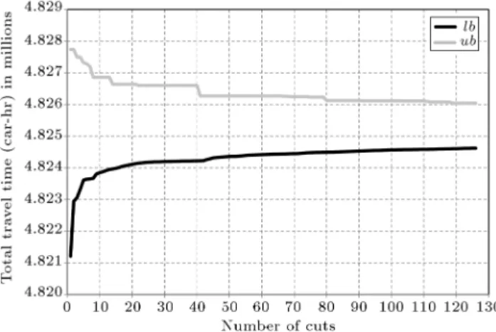
Figure 6 illustrates the values of the lower and upper bounds for the objective function, i.e., total travel time, obtained by the proposed algorithm for the Iranian rail network. The algorithm hits the one-hour time limit after adding 128 cuts and reaches the relative gap as equal to 0.034%, which is acceptable for the real-sized problem. The optimal value of model (P ) with the deterministic data was approximately 4.3 million car-hr, and the optimal value of the robust model was approximately 4.8 million car-hr, which is roughly a 10% increase; the robust solution also guarantees the validity of Constraints (12) and (13) with a probability of more than 0.98. Using the values of time, the
Figure 6. The value of lower and upper bounds for Iran rail network versus number of cuts.
economic benets of a deterministic solution can be quantied to compare it to the robust solution. It has been reported that the value of time for freight rail transportation is approximately 34 dollars (30 euros) per ton-hr in Europe [42]. Therefore, the price of robustness against uncertainty is approximately 425 million dollars in the three-month time horizon (where net car load is 25 tons).
The optimal solution to the robust model involves 1855 selected blocks and 1937 selected blocking paths, while the optimal solution to the deterministic model involves 1822 selected blocks and 1903 selected blocking paths. To emphasize the dierence between the opti-mal solutions of the deterministic and robust models in detail, the optimal solutions for block variables and ow variables from the two models are given in Table 3. For the sake of convenience in showing the results, the optimal solutions for the deterministic
Table 3. The comparison of the optimal solutions for deterministic and robust models.
Condition Number of cases happened za;D= 1 and za;R= 1 1270
za;D= 0 and za;R= 1 585
za;D= 1 and za;R= 0 552
vk;D
q > 0 and vk;Rq > 0 943
vk;D
q = 0 and vk;Rq > 0 994
vk;D
q > 0 and vk;Rq = 0 960
model are denoted by za;D and vk;D
q , and the optimal
solutions for the robust model are denoted by za;Rand
vk;R
q . For block variables, 1270 blocks were common
in the optimal solution of both models; however, 1137 blocks were not involved in the optimal solution of either model. For ow variables, 934 paths for the robust model were also involved in the deterministic model; however, 960 paths in the robust solution were equal to zero that were positive in the deterministic solution. This observation shows that the robust solution includes more paths than the deterministic solution does, which is also illustrated in [43,44] for the shortest robust path problem.
Figure 7 illustrates the number of blocking paths with volumes greater than the amount of ow shown on the horizontal axis. For example, consider the value of 5000 cars from the horizontal axis; then, the corresponding values on the vertical axis indicate the numbers of blocking paths with volumes greater than 5000 cars. This gure illustrates that, when moving from left to right on the horizontal axis, the deterministic line meets the robust line at a point in
the middle. It can be derived from the gure that the optimal solution to the deterministic model consists of more blocking paths with a larger volume. In partic-ular, the deterministic model yields four paths with volumes greater than 6000 cars; however, the optimal solution to the robust model has only one path with a volume greater than 6000 cars. However, this gure also suggests that the robust solution includes more blocking paths with less volume than the deterministic model. The authors also generated similar gures for dierent networks, and found that these gures follow the same trends.
6. Conclusion
The railroad blocking problem is an important issue at the tactical planning level. This problem includes identifying the list of visited classication yards for each shipment to improve the performance of car shipping while satisfying railway restrictions. Because the blocking parameters change monthly, they greatly aect the quality of the deterministic solution and can possibly render this solution meaningless in practice. Thus, the blocking plan must be re-optimized for new realizations of uncertain parameters; then, the next stage problems (such as train scheduling) should also be re-optimized. A methodology addressing this need is robust optimization [26], which produces a solution immunized against uncertain data. The robust model is an optimization program with continuous ow vari-ables, integer block varivari-ables, and nonlinear functions in the constraints. To solve the program, we developed a specialized branch-and-cut algorithm. This method is viewed as a generalization of the branch-and-bound method, with additional cuts generated on eligible branches of the branch-and-bound tree. To test the eciency of the proposed algorithm, the results of the proposed algorithm were compared with the optimal solution found by GAMS on 14 dierent instances. We observed that the proposed algorithm solved all instances optimally within one hour. However, GAMS could only solve 2 of the 14 instances optimally within one hour, and it was not able to nd a feasible solution for 8 of the 14 over one hour. Finally, the proposed algorithm was applied to a real-sized blocking problem. It was shown that, by ignoring 10% of the objective function of the deterministic model, which is approximately 425 million dollars for a three-month horizon time, we were able to develop an optimal solution that was immune to data uncertainty with a probability of more than 0.98. In addition, the optimal solution of the robust model was compared with that of the deterministic model, and our investigation showed that there is a fundamental dierence between the optimal values of the block and path variables for the two models.
References
1. Crainic, T.G. and Laporte, G. \Planning models for freight transportation", Eur. J. Oper. Res., 97, pp. 409-438 (1997).
2. Crainic, T.G. \Service network design in freight trans-portation", Eur. J. Oper. Res., 122, pp. 272-288 (2000).
3. Assad, A.A. \Modelling of rail networks: Toward a routing/makeup model", Transport Res. B-Meth, 14, pp. 101-114 (1980).
4. Fugenschuh, A., Homfeld, H., and Schulldorf, H. \Single-car routing in rail freight transport", Transport Sci., 49, pp. 130-148 (2013).
5. Barnhart, C., Jin, H., and Vance, P.H. \RailRoad blocking: A network design application", Oper. Res., 48, pp. 603-614 (2000).
6. Bontekoning, Y. and Priemus, H. \Breakthrough in-novations in intermodal freight transport", Transport Plan Techn., 27, pp. 335-345 (2004).
7. Bodin, L.D., Golden, B.L., Schuster, A.D., and William, R. \A model for the blocking of trains", Transport Res B-Meth, 14, pp. 115-150 (1980). 8. Marn, A. and Salmeron, J. \Tactical design of rail
freight networks. Part I:Exact and heuristic methods", Eur. J. Oper. Res., pp. 26-44 (1996).
9. Lin, B.-L., Wang, Z.-M., Ji, L.-J., Tian, Y.-M., and Zhou, G.-Q. \Optimizing the freight train connection service network of a large-scale rail system", Trans-portation Research Part B: Methodological, 46, pp. 649-667 (2012).
10. Newton, H.N., Barnhart, C., and Vance, P.H. \Con-structing railroad blocking plans to minimize handling costs", Transport Sci., 32, pp. 330-345 (1998). 11. Keaton, M.H. \Designing optimal railroad
operat-ing plans: Lagrangian relaxation and heuristic ap-proaches", Transportation Research: Part B, 23, pp. 415-431 (1989).
12. Hasany, R.M., Shafahi, Y., and Kazemi, S.F. \A com-prehensive formulation for railroad blocking problem", ECMS, pp. 758-763 (2013).
13. Ahuja, R.K., Jha, K.C., and Liu, J. \Solving real-life railroad blocking problems", Interfaces, 37, pp. 404-419 (2007).
14. Martinelli, D.R. and Teng, H. \Optimization of railway operations using neural networks", Transport Res C-Emer, 4, pp. 33-49 (1996).
15. Yaghini, M., Momeni, M., Sarmadi, M., Seyedabadi, M., and Khoshraftar, M.M. \A fuzzy railroad blocking model with genetic algorithm solution approach for Iranian railways", Appl. Math. Model, 20, pp. (2015). 16. Yue, Y., Zhou, L., Yue, Q., and Fan, Z. \Multi-route railroad blocking problem by improved model and ant colony algorithm in real world", Comput. Ind. Eng., 60, pp. 34-42 (2011).
17. Yaghini, M., Ahadi, H.R., Barati, E., and Saghian, Z. \Tabu search algorithm for the railroad blocking problem", J. Transp. Eng.-ASCE, 139, pp. 216-222 (2012).
18. Ahuja, R.K., Cunha, C.B., and Sahin, G. \Network models in railroad planning and scheduling", Tut. Oper. Res., 1, pp. 54-101 (2005).
19. Voll, R. and Clausen, U. \Branch-and-price for a European variant of the railroad blocking problem", Electronic Notes in Discrete Mathematics, 41, pp. 45-52 (2013).
20. Yaghini, M., Rahbar, M., Karimi, M., and Khoshkroudian, M. \A branch-and-price algorithm for solving the railroad blocking problem", International Journal of Engineering Science (2008-4870), 25, pp. 99-108 (2014).
21. Yang, L., Gao, Z., and Li, K. \Railway freight transportation planning with mixed uncertainty of randomness and fuzziness", Appl. Soft Comp., 11, pp. 778-792 (2011).
22. Gao, Y., Yang, L., and Li, S. \Uncertain models on railway transportation planning problem", Appl. Math. Model, 40, pp. 4921-4934 (2016).
23. Meng, Q., Hei, X., Wang, S., and Mao, H. \Carrying capacity procurement of rail and shipping services for automobile delivery with uncertain demand", Trans-port Res. E-Log, 82, pp. 38-54 (2015).
24. Milenkovic, M.S., Bojovic, N.J., Svadlenka, L., and Melichar, V. \A stochastic model predictive control to heterogeneous rail freight car eet sizing problem", Transport Res. E-Log, 82, pp. 162-198 (2015). 25. Jin, H., Designing Robust Railraod Blocking Plans,
Massachusetts Institute od Technology (1998). 26. Ben-Tal, A. and Nemirovski, A. \Robust solutions
of Linear Programming problems contaminated with uncertain data", Math. Prog., 88, pp. 411-424 (2000). 27. Prekopa, A., Stochastic Programming, Springer
Sci-ence & Business Media (2013).
28. Wong, W.G., Niu, H., and Ferreira, L. \A fuzzy method for predicting the demand for rail freight transportation", J. Adv. Transport, 37, pp. 159-171 (2003).
29. Carvalho, G., Methodology for Railway Demand Fore-casting Using Data Mining, SAS Global Forum (2007). 30. Gorman, M.F. \Statistical estimation of railroad con-gestion delay", Transport Res. E-Log, 45, pp. 446-456 (2009).
31. Matas, A., Raymond, J.L., Gonzalez-Savignat, M., and Ruiz, A. \Predicting the demand: Uncertainty analysis and prediction models in Spain", Work-ing Paper in Economic Evaluation of Transportation Projects, pp. 1-31 (2009).
32. Dong, Y. \Modeling rail freight operations under dierent operating strategies", PhD Thesis, MIT, Cambridge, MA (1997).
33. Birge, J.R. and Louveaux, F., Introduction to Stochas-tic Programming, Springer (2011).
34. Soyster, A.L. \Convex programming with set-inclusive constraints and applications to inexact linear program-ming", Oper. Res., 21, pp. 1154-1157 (1973).
35. Ben-Tal, A. and Nemirovski, A. \Robust convex op-timization", Mathematics of Operations Research, 23, pp. 769-805 (1998).
36. Seref, O., Ahuja, R.K., and Orlin, J.B. \Incremental network optimization: Theory and algorithms", Oper. Res., 57, pp. 586-594 (2009).
37. Han, J., Lee, C., and Park, S. \A robust scenario ap-proach for the vehicle routing problem with uncertain travel times", Transport Sci., 48, pp. 373-390 (2013). 38. Smith, J.C., Ahmed, S., Cochran, J.J., Cox, L.A.,
Ke-skinocak, P., Kharoufeh, J.P., and Smith, J.C. \Intro-duction to robust optimization", Wiley Encyclopedia of Operations Research and Management Science, John Wiley & Sons, Inc. (2010).
39. Nemhauser, G.L. and Wolsey, L.A. \Integer program-ming and combinatorial optimization", W., Chich-ester, G.L. Nemhauser, M.W.P. Savelsbergh, and G.S. Sigismondi, Constraint Classication for Mixed Integer Programming Formulations, COAL Bulletin, 20, pp. 8-12 (1988).
40. Lee, J. and Leyer, S., Mixed Integer Nonlinear Pro-gramming, Springer Science & Business Media (2011). 41. ILOG, CPLEX OPTIMIZATION, INC. 2009. Using
the CPLEX Linear Optimizer.
42. Van Essen, H., Boon, B., den Boer, L., Faber, J., van den Bossche, M., Vervoort, K., and Rochez, C., Marginal Costs of Infrastructure Use - Towards a Simplied Approach, Delft (2003).
43. Bertsimas, D. and Sim, M. \Robust discrete optimiza-tion and network ows", Math. Prog., 98, pp. 49-71 (2003).
44. Ben-Tal, A., El Ghaoui, L., and Nemirovski, A., Robust Optimization, Princeton University Press, New Jersey (2009).
Appendix
Ben-Tal and Nemirovski [26] introduced the following methodology for generating the robust formulation from linear model while the technological coecient are uncertain. Consider the following optimization problem [26]:
(AP 1) minXn
i=1
cixi; (A.1)
s.t.
n
X
i=1
~aijxi bj; j = 1; ; m; (A.2)
Suppose that, in constraint j, ~aij = (1+"ij)jaijj where
ij is the independent random variables symmetrically
distributed in interval [ 1; 1], " is the tolerance aect-ing ~aij, and jaijj is the average value of ~aij. Ben-Tal
and Nemirovski [26] proved the following theorem to generate the robust formulation of (AP 1).
Theorem. Let ^x be the optimal solution to the following optimization problem:
(AP 2) minXn
i=1
cixi; (A.4)
s.t.
n
X
i=1
aijxi+ n
X
i=1
" jaijj yij+ "j
v u u tXn
i=1
a2
ijzij2 bj;
j = 1; ; m; (A.5)
yij xi zij yij; i = 1; ; n;
j = 1; ; m; (A.6)
li xi ui; i = 1; ; n; (A.7)
yij 0; i = 1; ; n; j = 1; ; m: (A.8)
Then, ^x is feasible for (AP 1) with probability (1 exp( 2
j=2)) for constraint j where j is a positive
parameter [26].
Proof: Let ^x be feasible for (AP 2). Then: Pr
" n X
i=1
~aijxi> bj
#
(a)
z}|{= Pr"Xn
i=1
(aij+ " jaijj ij) xi> bj
#
= Pr " n
X
i=1
aijxi+ n
X
i=1
" jaijj xiij > bj
#
(b)
z}|{= Pr"Xn
i=1
aijxi+ n
X
i=1
" jaijj xiij
+
n
X
i=1
" jaijj yijij n
X
i=1
" jaijj yijij > bj
#
= Pr " n
X
i=1
aijxi+ n
X
i=1
" jaijj (xi yij) ij
+Xn
i=1
" jaijj yijij > bj
# (c) z}|{ Pr " n X i=1
aijxi+ n
X
i=1
" jaijj zijij
+Xn
i=1
" jaijj yijij > bj
#
(d)
z}|{ Pr
2 4Xn
i=1
" jaijj zijij > j"
v u u tXn
i=1
a2 ijz2ij
3 5
(e)
z}|{= Pr 2 4Xn
i=1
ijij > j
v u u tXn
i=1 2 ij 3 5 (f)
z}|{= Pr"Xn
i=1
ijij> j
#
(g)
z}|{
exp 2
j E ( exp ( j n X i=1
ijij
))
(h)
z}|{= exp 2
j
Yn
i=1
E fexp fjijijgg
(i)
z}|{= exp 2
j Yn i=1 "1 X l=0
(jij)2l
(2l)! #
(j)
z}|{= exp 2
j
exp 2 j=2 n X i=1 2 ij ! (k)
z}|{= exp 2
j
exp 2 j=2
= exp 2
j=2
:
In (a), we substitute ~aij into (1 + "ij)jaijj, in (b) we
add and subtract Pni=1"jaijjyijij, in (c) we consider
xi yij zij, in (d) we consider Pni=1aijxi +
Pn
i=1"jaijjyij + "jqPi=1n a2ijz2ij bj, in (e) we
substitute ij into jaijjzij, in (f) we assume the case of
Pn
i=12ij = 1, in (g) we use the Tschebyshev inequality,
in (h) we use independence of ij, in (i) we use the
denition of expected value of EXP and symmetry of the distribution of ij = [ 1; 1], in (j) we use Taylor
series, and in (k) we assume the case ofPni=12
ij= 1.
In the above discussion, Only the uncertainty which is inherent in the technological coecients is considered for model (AP 1) (used by Ben-Tal and Nemirovski [26]). However, the blocking problem involves uncertainty in both the objective function and right-hand side of the constraint. In the paper, we applied some modications to the uncertain model to
adopt the idea of Ben-Tal and Nemirovski [26] (stated above) to present the robust formulation for blocking problem.
Biographies
Reza Mohammad Hasany received his Bachelor of Science degree in Civil Engineering in 2007 and his Master of Science degree in Transportation Planning in 2010 from Sharif University of Technology, Tehran, Iran. Currently, He is a Doctoral Student at Depart-ment of Civil Engineering in Sharif University of Tech-nology. In his PhD's thesis, he worked on modeling and solution algorithm for the railroad blocking problem. His research interests include mathematical
program-ming, large-scale optimization, and optimization under uncertainty.
Yousef Shafahi obtained his BS from Shiraz Uni-versity, Shiraz, Iran; MS from Isfahan University of Technology, Isfahan, Iran; and PhD from University of Maryland, College Park, MD, USA. He joined the Department of Civil Engineering in Sharif University of Technology, Tehran, Iran as an Assistant Professor in 1998 and is now a Professor and the Head of Transportation Division group at this Department. His research interests are urban transportation planning; road, rail, and air transportation; transit networks de-sign and scheduling; applications of operation research, soft computing and simulation in transportation.