FLOW THROUGH RIGID STRUCTURES
Madeleine Braye Department of Mathematics
March 26, 2019
ABSTRACT
The movement of very small aquatic organisms depends heavily on the fluid around them, as they are easily influenced by the dynamics of their system. Therefore, current research seeks to understand the complex fluid dynamics of these small scale systems to better understand how these dynamics can affect the locomotion. Numerical models of these environments are challenging to create due to the level of detail required and the massive number of computations that must be solved, but new improvements in scientific computing have recently made these models more feasible. In this paper, we largely seek to study rooted aquatic vegetation consisting of macrophytes, and their effects on the fluid dynamics of their system and the distribution of zooplankton within it. To successfully research the movement of organisms and particles in these aquatic ecosystems, it is necessary to understand how variations in macrophytes affect the fluid dynamics around them and be able to successfully model these dynamics. In this project, fluid flow through rigid physical models of aquatic vegetation is analyzed to quantify the flow profiles caused by varying the height and density of macrophyte configurations. The dynamics are modeled in several different ways to evaluate the computational cost and accuracy of each model, with the intention of supporting a later project assessing flexible macrophytes and their impact on the distribution of zooplankton.
Keywords immersed boundary method·numerical simulation·fluid dynamics
1
Introduction
Complex and flexible vegetation occurs frequently throughout our ecosystems, and significant amounts of research depend on our understanding of the fluid dynamics around and through these structures. Numerical simulations of the impact various configurations of these and other biological structures have on flow are difficult to create, but have numerous applications, ranging from small scale interactions of lung fluid with cilia [23] to large scale systems such as wind flow through forests and its effects on pollen dispersal [22]. The dynamics of these environments are very convoluted, as they depend on a large variety of factors and vary widely throughout the system. However, they have a massive impact on the environment around them, and, for this reason, accurate modeling techniques for these structures and their environments is vital.
the complexity. Numerical solvers have difficulty solving systems of this computational cost and size, as the distinct interactions require a massive number of operations to accurately model the movement of the fluid through the environment. However, recent developments in research comput-ing, combined with adapted numerical solving methods, have increased the feasibility of creating well-structured models of these environments, and allow us to investigate the small spatial scale flow of these systems.
Slow moving flows with unobstructed paths generally experience steady-streaming, sheet-like flow, and when the flow is disrupted by obstructions it can become turbulent, with the velocity profile of the flow field developing unpredictable eddies and vortices. However, it is important to note that unpredictable flow patterns such as nonturbulent eddies may still form if the Reynolds number is sufficiently small (on the order of 1000 or less), adding three-dimensionality to the flow fields. Turbulent flow and other three-dimensional patterns vary widely within the system in contrast to smooth-streaming flow, creating small-scale, intricate flow fields. Furthermore, when both of these types of flows exist within an ecosystem, they interact and can cause areas to vary between smooth streaming and vortical flow. In aquatic ecosystems such as kelp forests and beds of macrophytes, the obstructions both strongly influence and are strongly influenced by their environment, and modeling the changes in the macrophytes and the fluid flow around them is difficult. However, the dynamics of these ecosystems have a strong impact on the small organisms and particles within them, which experience their environment on a small spatial scale. The movement of these organisms and particles depends on their interactions with the patterns of flow; for this reason, most research on these topics depends on an accurate and detailed understanding of the fluid dynamics of these systems.
A significant amount of current research involves the movement of organisms and particles within systems such as these, and all cite the need for improved modeling techniques to increase understanding of aquatic ecosystems. [20, 18, 33] In a recent project proposal, Miller et al seek to research the impact of aquatic environments on the locomotion and dispersal of plankton. Since their behavior is on such a small scale, it is vital to understand the dynamics of their environment. Therefore, to develop this research, we first need to understand how the density, height, and rigidity of macrophytes affect the flow field within and around the vegetation bed and develop accurate and detailed analytic and numerical models of the fluid flow through complex structures.
Although studies of specific applications suggest that variations of factors such as height, density, and Reynolds number of configurations of aquatic vegetation have large effects on the three-dimensional flow produced by these structures [16, 8, 34], detailed quantitative data has not been obtained. This suggests that successful numerical models of these environments must also be adaptable, as they must account for small variations of vegetation throughout the ecosystem, which may have large effects on the velocity profile.
This research seeks to expand our understanding of how varied configurations of these simpli-fied cylindrical arrays at intermediate Reynolds numbers affect the flow field of their environment, as well as evaluating the level of detail and computational cost of various modeling techniques that can be used to simulate these systems. The results of this project will be used to to supplement the larger project in progress by the Miller lab.
1.1 Challenges in Numerical Modeling
Small-scale flow through these types of structures creates complex velocity profiles that are difficult to numerically model for a variety of reasons. One of the most significant reasons these models are challenging to create is the computational cost of numerically solving the Navier-Stokes equations. The flow properties of these environments vary widely based on a variety of factors, and quantifying the interactions of these factors with their environment and each other requires a massive amount of operations, all of which need to be evaluated at each time step of the model. This complexity is often intractable, requiring most models of these environments to ignore the detailed, three-dimensional flow in favor of simulating the bulk flow of the system.
fluid, the pressure of the system, and the size of the environment. The structural equations and geometries can be very complex, requiring the mesh to be adaptable to the local dynamics. These factors can also change over time, requiring the mesh to adapt to changing variables. Updating these domains at each time step requires a large amount of computations, often to the detriment of the accuracy of the simulation.
Accurate models must also consider fluid structure interactions. Fluid structure interaction (FSI) problems combine computational fluid dynamics with computational structural dynamics to numerically solve the equations predicting the movement of both the fluid domain and the structural domain. Fully coupling the interactions of the structure and the fluid can involve remeshing the computational flow domain at each time step in reaction to the deformation of the structure and can involve tens of millions of unknowns in certain environments [9]. Models that take the FSI’s of the system into account introduce a massive increase in the computational cost of the model and must prioritize computational efficiency in their numerical modeling methods.
The numerical methods and computational infrastructure required by these simulations have only recently become available with advancements in computing and numerical algorithms, and the use of these techniques has introduced many new options in the research of these systems. By creating accurate and detailed models of the entire systems on a small scale, we can better understand not only the dynamics of the environment, but also how organisms and particles within the systems behave and interact with the world around them.
1.2 Reynolds number
The Reynolds number (Re) is an important dimensionless variable which describes the relative inertial to viscous forces in the flow field. This number is given by
Re= ρU L
µ , (1)
whereρis the viscosity of the fluid,µis the dynamic viscosity of the fluid,U is a characteristic velocity (in this project we use the free stream velocity of the flow field), andLis a characteristic length scale.
An important note here is that the Reynolds number is affected by the introduction of obstruc-tions to the flow. Because of this we used two differentRes in this project, one for the bulk flow of the system and one at the level of the individual macrophyte models. For the bulk flowRe, we used the height of the computational domain as the characteristic length scaleL, in this case the height of the flow tank. At the level of the cylinders, we used a diameter basedReto describe the relative importance of inertial and viscous effects on the small scale system, which can be calculated by
Red=
ρU D
µ , (2)
whereDis the diameter of the cylinders.
and more complex flow patterns. This pattern continues until very highRes (Re > 105), where the
flow becomes turbulent and chaotic. The vortices formed by each cylinder interact with each other in various ways, developing intricate flow patterns that change throughout the array and are very difficult to fully resolve.
Figure 1: (left) Graph depicting the change in the drag coefficient of cylinders as the diameter-basedRe is increased. (right) Flow profiles produced by fluid flow past a cylinder at different diameter-basedRes. [4]
1.3 Analytical porous models
Most analytical models used in simulating flow involve large scale averaging systems, which standardize the dynamics and often ignore the detailed three-dimensional fluid flow that occurs within the structures in favor of studying the bulk flow of the system [21, 1, 24]. For example, many models use the Brinkman equations to describe the flow through macrophytes, seen in detail in the methods section.
1D analytical models have been developed using Darcy’s Law, its generalization to the Brinkman law, and the Darcy-Forchheimer law to model the flow of fluid through systems of aquatic vegetation. These methods have been used to research the flushing of plankton and pollen particles from sea grass meadows and kelp forests [10, 15] as well as the distribution of zooplankton which are using the small scale local velocity field to change direction within their ecosystem [13, 29, 17]. Modified Brinkman equations using a Cantor-Taylor brush configuration [31, 30] have also been used to consider three regions of flow: a dense layer, a sparse layer, and a layer free of obstructions.
These porous models have significant limitations. By design, they represent the fluid field as homogenized steady flow, assuming there is no flow into or out of the layer and averaging out the eddies and vortices formed by the interaction between the flow and the cylinders. The error introduced by the homogenization of the porous layer will be proportional to the amount of flow in the third dimension [26], and so these averaging models introduce a significant amount of error within the porous layer. In the research of Strickland et al, [32], it was found that while these equations are accurate for the bulk flow of the system, they do not provide an adequate amount of detail at the small scale as seen in newer numerical models. Therefore models with higher accuracy within the vegetative layer are required to definitively study the movement of organisms and particles in the system.
1.4 Past research
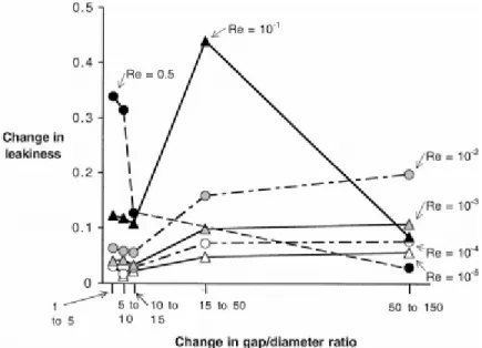
defined as the ratio of the volume of liquid that flows through the gap in a unit of time to the volume of liquid that would flow at freestream velocity through a space of that width if there were no obstacles present [19]. She found that, at lowRes (10−5 < Re <0.5), the spacing of cylinders has
a strong effect on the leakiness of the model, as seen in figure 2. If the spacing between cylinders is large, they function as a leaky sieve, influencing the flow but not obstructing it, whereas if the gap is small, they act as a solid paddle, redirecting the flow. In this project, we explore the effects of large configurations of structures, involving hundreds of cylinders arranged in a group placed into fluid flow. Based on Koehl’s previous work, we expect the configurations of macrophytes that are very dense in spacing to act similarly to a solid, redirecting fluid flow around the array as a whole, whereas less dense configurations may allow fluid flow to filter through the model and flow around the cylinders.
Figure 2: Relationship between spacing of cylinders and leakiness of configuration at lowRes. [19]
In previous work, Strickland et al [32] detailed the flow within biological filtering layers and solved the associated fully coupled fluid structure interaction problem for simplified structures of a line or array of up to 16 cylinders using the immersed boundary method. This project compared these fully resolved models to a Brinkman model, as well as experimental PIV data. This project supported the results found by Koehl on the effects of structures on fluid flow and found that the level of detail found in these models was not adequately seen in averaging analytical models. They found that the Brinkman model adequately described the averaged flow profiles and shear stresses as seen in the PIV data but the numerical simulations of the environment revealed more complex flow patterns that were lost in the averaging models. In this project, we look to expand that work to cover more complex systems of structures and investigate their effects on flow patterns. Furthermore, we will quantify how the average flow changes as it penetrates a long array of cylinders and also how additional rows of cylinders increase the three-dimensionality of the flow.
1.5 Project Goals
• A one-dimensional Brinkman model of flow through porous layers is used to evaluate the average flow of the system. We expect this to accurately model the bulk flow of the system but provide inadequate levels of detail for the complex fluid flow.
• Particle image velocimetry (PIV) is used to measure flow around physical models of macro-phytes. This method also has difficulty fully resolving the flow within the macrophyte region, due to the opacity of the models.
• Fully resolved three-dimensional flow through the macrophytes is simulated using the IBAMR framework.
• Stationary flow through the cylinders is simulated using COMSOL multiphysics sofware.
The goal is to evaluate the bulk flow of the system experimentally using PIV and confirm the Brinkman model while verifying that they provide insufficient detail of the fully resolved flow fields. Then, the numerical models will be used to investigate the detailed effects of the physical models on the resulting velocity profile of the system.
2
Methods
2.1 Experimental setup
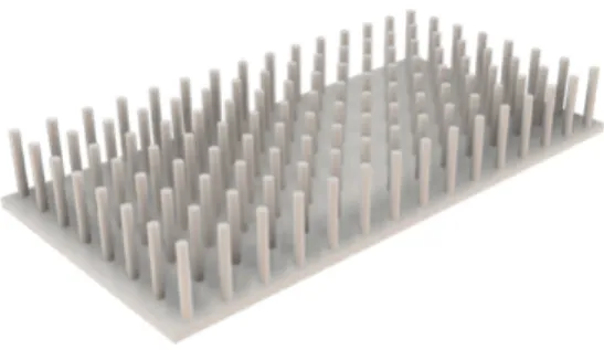
Macrophytes in the system were modeled by rigid cylinders arranged in a grid, as seen in Figure (3). For this experiment we created three different variations of models. For all models, the base consisted of a 7.5 x 10 x 0.25 cm rectangular prism, bonded to rigid cylinders of 0.25 cm in diameter and of varying heights. The models were built as one component in Autodesk Fusion 360 [3] and were 3D printed on their sides using the uPrint machine. The models used for particle image velocimetry were lightly spray painted black.
Figure 3: Macrophyte model of 8x15 cylinders and 2 cm height
Figure 4: Mesh of the 8x15 model of 2 cm height produced by Bolt and used in the numerical simulations
• The least dense model consisted of cylinders arranged in an 8 x 15 evenly spaced grid. There was a 0.75 cm space between each cylinder in both the x and y direction.
• The medium dense model consisted of cylinders arranged in a 10 x 20 grid. These had a 0.5 cm space between each cylinder.
• The densest model consisted of cylinders arranged in a 15 x 30 grid. These had a 0.25 cm space between each cylinder.
Each variation of the model was printed with heights of 1, 2, and 3 cm to study the effects of the different configurations on the resulting velocity profile. The files used to create the models were then meshed using the software Bolt [7] so that they could be imported into the numerical modeling software and used to simulate the macrophytes in the numerical models.
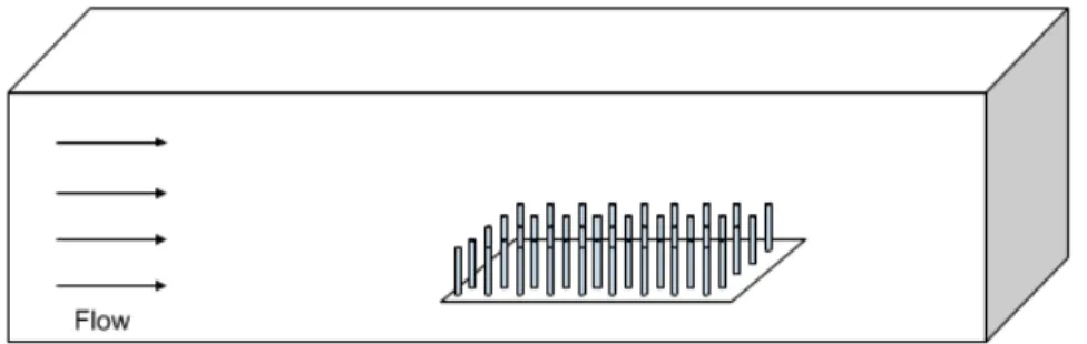
To get the experimental data, the physical models were placed at the center of the bottom of an optically accessible plexiglass flow tank, and kept in place using marine putty as if submerged and rooted. The flow tank is 8 cm in width and height and 320 cm in length, as depicted in Figure 5. Fluid was pushed through filtering layers on either end of the tank by a propeller attached to a variable speed motor to create parabolic flow through the channel at a maximum rate of 68 mm/s. Based on the experimental setup, we can calculate theRes of the system. Here we considered the
Figure 5: Experimental set up of macrophyte models in the flow tank
viscosity of the fluidρ= 1020kg/m3, the dynamic viscosityµ= 0.00089m2/s, the characteristic
velocityU = 0.068m/s, the characteristic length L = 0.08m, and the diameter of the cylinders D= 0.0025m. This gives us the following calculations:
Re= 1020
kg
m3 ×0.068
m
s ×0.08m
0.00089ms2 = 6235
Red=
1020mkg3 ×0.068
m
s ×0.0025m
0.00089ms2 = 195
TheseRes fall within the interval of10< Re <105, and are expected to induce vortex shedding
around the cylindrical structures.
2.2 PIV
Experimental results of the velocity flow field of the system were obtained using particle image velocimetry (PIV), in which tracer particles dispersed throughout the fluid are illuminated with a laser sheet. The motion of these particles is then recorded and processed using correlation based techniques to develop the velocity vector field of the fluid flow. This produces a two-dimensional vector profile of the velocity of the fluid flow. Detailed reviews of PIV can be found here [2, 35].
simulations.
The figures provided in this paper were obtained using time-averaged PIV. The laser sheet for the measurements was generated from a 50 mJ double-pulsed Nd:YAG laser manufactured by Continuum Inc., which emits light at a wavelength of 532 nm with a maximum repetition rate of 15 Hz. The laser beam was converted into a planar sheet approximately 3 mm thick using a set of focusing optics. The laser sheet was located in the x-y plane along the center of the flow tank. The time interval of separation between the two images in an image pair was held constant at 0.1 s throughout all experiments. A 14 bit CCD camera (Imager Intense, LaVision Inc.) with a 1376 x 1040 pixel array was used for capturing images. Uniform seeding of the fluid was accomplished by inserting 10 micron hollow glass spheres into the flow tank and mixing to achieve a near homogenous distribution prior to each experiment. Davis 7.0 software was used for processing the raw images. For each PIV run, 20 images were recorded for processing, resulting in a minimum of 10 velocity vector fields from which to generate the mean flow field and statistics.
2.3 1D Analytical Brinkman model
Figure 6: Physical setup for the Brinkman model. Region I contains the shear flow, whereα2 = 0,
while Region II involves the turbulent flow through the porous layer, whereα2 >0.
A future goal of this project is to develop a Brinkman model for this setup, considering two main regions, depicted in Figure (6). Region I consists of the main channel, with unobstructed parallel shear flow, which is bounded at the bottom by Region II, describing the flow of the fluid through the porous layer. The inverse of the hydraulic permeability in the region of unobstructed flow should be 0, while the region with obstructions has a non-zero α, changing the Brinkman equations used to represent the velocity profile of the region.
ρ(ut(x, t) +u(x, t)· ∇u(x, t)) =∇p(x, t) +µ∇2u(x, t) +F(x, t) +α(x)µu(x, t) (3)
To obtain modeling equations, we first rewrite the two-dimensional Brinkman equation:
∂u ∂t +u
∂u ∂x +v
∂u ∂y =−
1
ρ ∂p ∂x +η(
∂2u ∂x2 +
∂2u ∂y2)−
α2
ρ µu (4)
∂v ∂t +u
∂v ∂x +v
∂v ∂y =−
1
ρ ∂p ∂y +η(
∂2v
∂x2 +
∂2v
∂y2)−
α2
withη = µρ. The flow in the model is considered to be steady, fully developed, and zero in the cross-stream direction, meaning that ∂u∂t = ∂u∂x =v = 0.
Region I: Using these assumptions, as well as assumingα2 = 0, the x-momentum equation (4)
in the free shear flow region simplifies to:
d2u dy2 =−
1
µ ∂p
∂x (6)
and the y-momentum equation (5) simplifies to
∂p
∂y = 0⇒p=p(x) (7)
These equations indicate that the fluid pressure is independent of the y-direction, and only changes in the x-direction.
To create the 1D model, we need to find a closed-form expression for the velocity of the flow field in this region. To obtain this, we integrated equation (6) iny, which produces the velocity gradient du dy = y µ dp
dx +A (8)
and then integrated again to give us
u(y) = y 2
2µ dp
dx +Ay+B (9)
To evaluate A and B, we have to use two boundary conditions.
Region II: to distinguish the velocity variable from the other region, we will useu∗ to represent the streamwise x-directional velocity within the model layer. Using equations (4) and (5), and assumingα2 >0, we get
d2u∗ dy2 =
1
µ dp dx +α
2u∗
(10)
The resulting second order differential equation can be converted into a set of two first-order differential equations by using a new variablewsuch that
du∗
dy =w (11)
which allows us to reduce equation (10) to
dw dy =
1
µ dp dx +α
2u∗
(12)
The redefinition ofwin equation (11) and equation (12) represent a two-dimensional system of non-homogenous, first order differential equations which can be further simplified into a homogenous system by defining a transformation foru∗.
˜
u∗ = (u∗+ 1
α2µ
dp dx)
which means
du˜∗
dy = du∗
dw dy =α
2u˜∗
This system can be written in matrix form as d dt ˜ u∗ w = 0 1
α2 0 u˜
∗ w
and solved using conventional linear algebra techniques to produce the following velocity profile for Region II:
˜
u∗(y) =Ceαy +De−αy
u∗(y) =Ceαy +De−αy− 1 α2µ
dp dx w(y) = αCeαy−αDe−αy
(13)
where the constants C and D will be evaluated using boundary conditions.
Consider the conditions of the system. We know velocity is a positive constant aty=b, for some b in the region, such that(U(b) > 0)and at the bottom, y = −a, the system has a no-slip condition so thatu(−a) = 0. Applying these conditions to equation (8), we get
b2 2µ
dp
dx +Ab+B =U >0 (14) Applying the no slip conditionu(−a) = 0to equation (13) produces
Ce−αa+Deαa = 1
α2µ
dp
dx (15)
Matching the velocitiesu(0) =u∗(0)at the change between regionsy= 0yields
B =C+D− 1 α2µ
dp
dx (16)
and matching the velocity gradients of the two regions produces the equation
A=αC−αD (17)
Solving equations (14), (15), (16), and (17) for constants C and D results in
C =
dp dx(−
1 2α
2b2 +αbe−αa−e−αa+ 1) +U α2µ
α2µ(αbe−2αa+αb−e−2αa+ 1)
D =
dp dx(
1 2α
2b2+αbeαa+eαa−1)−U α2µ
α2µ(αbe2αa+αb+e2αa−1)
Using equations (16) and (17), we can define the other constants in terms of C and D, and then these constants can be applied to equations (8) and (9) to find the closed-form expression for the velocity of the flow field in this region.
2.4 Immersed Boundary Method
The immersed boundary method [27] is used in this paper to solve the fully coupled fluid-structure interaction problem of viscous flow moving between cylinders. The method uses the incompressible Navier-Stokes equations to describe the fluid, elasticity equations to describe the boundary, and integral equations with delta function kernels to describe the interactions between the two. This method has been proven for successful use in various applications, including incompressible flows with complex and moving geometries [14].
This method describes the fluid using a fixed Cartesian mesh, with the immersed elastic boundary defined on a curvilinear mesh that can move freely through the Cartesian mesh and is not constrained to adapt to it in any way.
The two-dimensional formulation of the immersed boundary method is shown below, and the three dimensional formulation follows mathematically. A full formulation of the three dimensional method can be found at Peskin [27].
The Navier-Stokes equations that represent incompressible, viscous fluid motion are shown below:
ρ
"
∂u
∂t(x, t) +u(x, t)· ∇u(x, t)
#
=∇p(x, t) +µ∆u(x, t) +F(x, t) (18)
∇ ·u(x, t) = 0 (19)
whereu(x, t)is the fluid velocity,p(x, t)is the pressure,F(x, t)is the force per unit area applied to the fluid by the immersed boundary, ρ is the fluid density and µ is dynamic viscosity. The independent variables are the timetand the positionx. An important note is that the variablesu, p, andFare all written in an Eulerian framework on the fixed Cartesian mesh,x.
The interaction equations between the fluid and the boundary are given by:
F(x, t) = Z
f(q, t)δ(x−X(q, t))dq, (20)
Xt(q, t) =u(X(q, t)) =
Z
u(x, t)δ(x−X(q, t))dx, (21)
where f(q, t) is the force per unit length applied by the boundary to the fluid as a function of Lagrangian position,q, and time,t,δ(x)is a two-dimensional delta function, andX(r, t)gives the Cartesian coordinates of the material point given by the Lagrangian parameter,q, at time,t. Equation (20) applies a singular force from the immersed boundary to the fluid through the external forcing term seen in Equation (18), while Eq. (21) interpolates the local fluid velocity at the boundary. This enforces the no-slip condition and the boundary is then moved at the local fluid velocity.
The forcing termf(q, t), seen in the integrand of Eq. (20), is specific to the application; in a simple case such as this one where the boundary motion is prescribed, the boundary points are tethered to target points in the domain. This holds the boundary nearly rigid, and then the equation describing the force applied to the fluid by the boundary is:
f(q, t) = ktarg(Y(q, t)−X(q, t)) (22)
wherektarg is the stiffness coefficient andY(q, t)is the prescribed position of the target boundary.
2.5 Hybridized immersed boundary finite element method
In the immersed boundary method, immersed structures are discretized as a collection of infinitely thin one-dimensional fibers. Structures are then constructed as systems of fibers which often exhibit anisotropic traits. Furthermore, there are not very many finite difference mesh generators, and therefore it can be difficult to discretize complicated two and three-dimensional boundaries into the IBAMR framework. For this reason, to solve the 3D numerical model, a hybrid finite difference/finite element approach of the immersed boundary method (IBFE) will be used, which was developed by Griffith et al. [12]. This method adopts standard Lagrangian finite element methods to discretize the structure while retaining finite difference methods to discretize the Eulerian fluid grid, described by the Navier-Stokes equations. Rather than describe individual Lagrangian point-to-point type deformation models with fiber models, IBFE builds upon the finite element framework to describe the Lagrangian body from a solid mechanics foundation. This allows us to describe isotropic materials for the structures and greatly increases the number of finite mesh generators available, as they are more common for use in solid mechanics where finite element methods are prevalent.
The IBFE equations are explained here in 2D, and are based on those of the traditional immersed boundary method. The extension of these equations into the third dimension are straightforward and are solved using the IBAMR software.
In this method the structure material coordinates are defined to beX = (X, Y) ∈S, where Srepresents the Lagrangian structure domain. The physical positions of(X)at timetis given by χ(X, t) ∈ Ω, whereΩis the region which contains the entire fluid-structure interaction domain. Therefore, the space occupied by the structure at timetisχ(S, t)⊂Ω. This formulation uses the Piola-Kirchhoff solid stress tensorP(s, t). This provides the current elastic deformation forces of the immersed structure in terms of its reference configuration. structural forces in the spatial configuration per unit area in the material configuration. If the material is hyperelastic, then there is an energy functionalW(F)of the deformation gradientF= ∂χ∂s, andPij = ∂∂WF
ij fori, j = 1, ..., d.
Pis related to the corresponding Cauchy stressσbyσ= 1JPFT, withJ =det(F). The equations
describing the interaction between the boundary and the fluid are then:
f(x, t) = Z
U
∇s·P(s, t)δ(x−X(s,t))∆s−
Z
∂U
P(s,t)N(s)δ(x−X(s,t))dA(s), (23)
∂X
∂t =
Z
Ω
u(x,t)δ(x−X(s,t))∆x=u(X(s,t),t) (24)
in whichF(s, t) = ∇s·P(s, t)is the Lagrangian interior elastic force density,T(s, t) =P(s,t)N(s)
is the Lagrangian transmission elastic force density, in whichN(s)is the exterior unit normal to ∂U and δ(x) = Qd
i=1δ(xi)is the d-dimensional delta function. In the interior of the immersed
body,∇x·σ(x, t) =
R
U∇s·P(s, t)δ(x−X(s,t))∆s. The transmission forceT(s, t)accounts
for traction-like forces at fluid-solid interfaces. These singular force layers must be balanced by discontinuities in the pressure and viscous shear stress at fluid-solid interfaces. These discontinuities may be handled by the conventional IB method [27].
2.6 Numerical setup: IBAMR
domain where high-resolution is not warranted.
For this project the Eulerian grid was locally refined near both the immersed boundaries and regions of vorticity where|ω| >0.50. This Cartesian grid was organized as a hierarchy of four nested grid levels; the finest grid was assigned a resolution ofdx = L/256. A 1:4 spatial step size ratio was used between each successive grid level. The Lagrangian spatial step resolution was chosen to be equal to the resolution of the finest Eulerian grid, e.f.,ds = L/256. The fluid was simulated as parabolic inflow with a maximum velocity of 68 mm/s and the back wall was simulated as equivalent parabolic outflow. The other four walls of the flow tank were simulated as having the no-slip boundary condition.
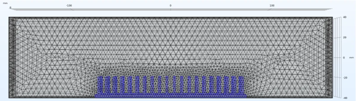
Figure 7: Adaptive refinement of mesh around the cylindrical models in COMSOL. Black mesh is of normal resolution, depicting the fluid domain, purple mesh is fine resolution, depicting the structural domain.
2.7 Numerical setup: COMSOL
In the COMSOL software we carried out the simulations using a single-phase laminar flow physics to solve a stationary study of the environment. The fluid domain was set to 80 x 320 x 80 mm and filled with liquid water while the cylindrical model was imported as an stl file and constructed out of iron. The front wall was given an inlet boundary condition of parabolic flow with an maximum velocity of 68 mm/s and the back wall was given an outlet condition with 0 pressure. The other 4 walls of the tank were given no-slip boundary conditions. Note here that the outflow boundary conditions are different between the IBAMR and COMSOL simulations. These differences will be resolved in future work. A free tetrahedral mesh was used for both domains; the mesh of the fluid domain was of normal resolution and calibrated for fluid dynamics while the mesh of the cylinders was fine and calibrated for general physics. Both can be seen in Figure 7, with the fluid domain meshed in black and the structural domain in purple.
3
Results
In this section we’ll explore the difference in the fluid dynamics generated by different macrophyte models. The goal of this section is to evaluate what methods are sufficient to describe the fluid dynamics through the cylindrical arrays, while incorporating the need for feasibility and accuracy.
3.1 PIV results
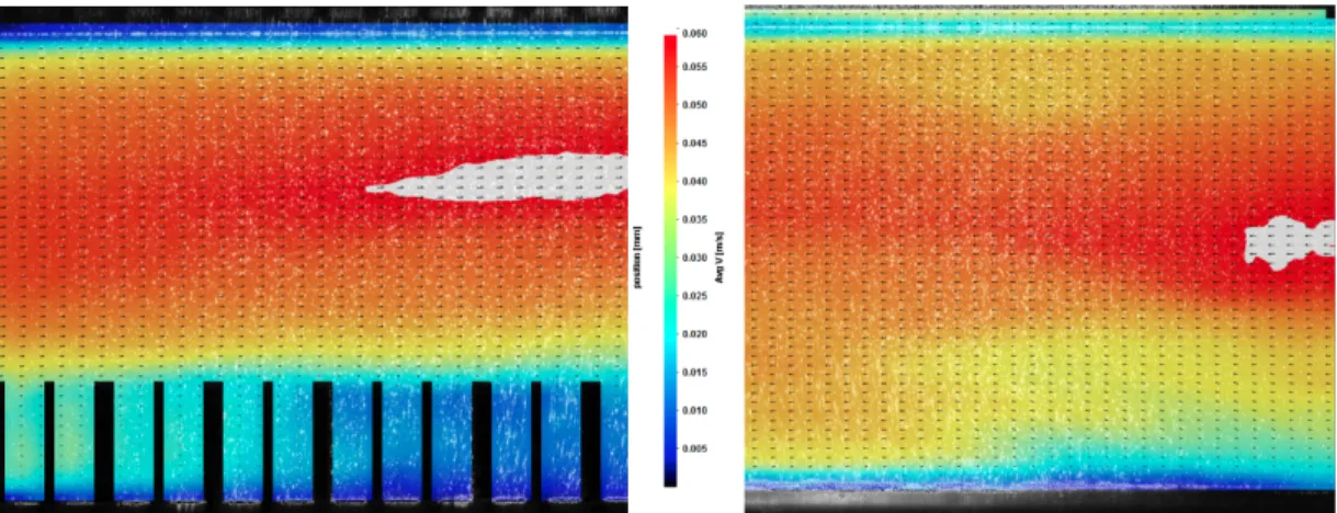
Figure 8: Averaged velocity profiles from the side view obtained by PIV analysis of a) fluid flow over the 10x20 2 cm array, and b) fluid flow through the empty flow tank. Flow is from left to right. Arrows depicting the direction of flow are normalized, with the color depicting the magnitude of the velocity. Maximum of velocity scale is white.
the structures strongly affect the generated flow fields. It is evident that as soon as the flow field begins to interact with the cylinders the three-dimensionality of the flow increases and disrupts the steady-streaming flow. Another interesting note is that this three-dimensionality is compounded with the continued rows of cylinders, creating slower flow patterns at the end of the model.
3.2 Fit of 1D Model to Experimental Data
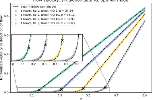
In previous research, Strickland et al. were able to match a 1D analytical Brinkman model to experimental data of fluid flow around cylinders of varying height with some accuracy. Figure 9 shows the best fitting Brinkman model coupled with the average velocity in the direction of flow for the various cylinder heights. The height of the cylinder is shown by the X, while the color lines display the experimental data and the dashed line represents the best-fitting Brinkman model. While the zoomed in section of the graph shows that the Brinkman model is not exact, it fits the data very closely. In future work, we will use the Brinkman model derived in the methods section and match it to the experimental data. Since the Strickland data pertains to one cylinder in flow, we expect it to be more difficult to find an accurate fit by a one-dimensional model, as the model will have a difficult time fully resolving the detailed fluid flow caused by a large array of cylinders.
3.3 IBAMR simulations
Figure 10 shows the pseudocolor plot of the magnitude of the velocity profile produced by fluid flowing at 0.068 m/s through the channel containing the model of medium density printed at a height of 2 cm. The figure shows steady-streaming flow passing smoothly over the top of the model, with significant velocity differences between the middle of the region and the top and bottom. After the fluid passes over the model, the fluid appears to change velocity, due to the three-dimensionality of the flow and fluid leaving the layer.
In Figure 11, you can see the detail in the fully resolved velocity vector field produced by IBAMR. This figure shows the three-dimensionality of the flow, as well as the formation of eddies that occurs at the beginning and end of the model. A large eddy is formed right after the end of the model, increasing the three-dimensionality of the flow and causing more mixing of the system.
Figure 9: Average velocity in the direction of the flow for various cylinder heights, compared with the best fitting Brinkman model. The top of each cylinder is marked with a black X. The best choice of porosity is given for each cylinder height in the figure legend. [32]
Figure 11: Side view of the velocity vector profile of the IBAMR simulation of flow through the medium density model at 2 cm of height. Flow is from left to right. Data taken on the yz-plane parallel to the direction of flow, through the middle of the array centered between two rows of cylinders (x=0, 0.25 cm away from each cylinder). Arrows show direction of flow and are normalized, with magnitude of velocity denominated by color. Cylinder mesh shown in black. The outflow condition is zero pressure rather than parabolic outflow.
array, reaching nearly 0 as it exits the model. It then spikes once more due to the eddy in the flow behind the array and experiences more irregular flow patterns. This type of detailed and irregular flow is generally very hard to compute, which increases the computational cost of the simulation.
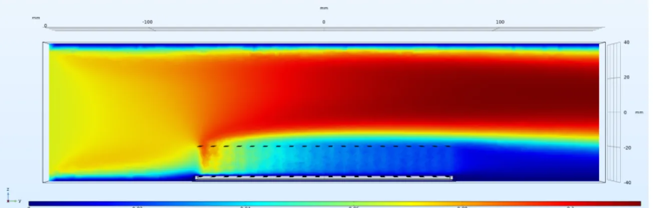
Figure 13: Pseudocolor plot of the magnitude of the side view of the velocity in the COMSOL simulation representing the fluid flow over the medium density cylinder model at a height of 2 cm. Flow is from left to right, magnitude of the velocity taken on the yz-plane in the middle of the cylindrical array (x=0).
3.4 COMSOL simulations
COMSOL simulations were used in this project to compare the variations in macrophyte models due to the large number of simulations required and the quick computational time of a stationary model. Figure 13 displays the side view of the magnitude of the velocity of the medium density model at 2 cm of height. When compared to Figures 10, 11, which depict the same simulation run by IBAMR, there are obvious differences between the IBAMR unsteady model and the COMSOL stationary model. To begin, much of the complex flow structures observed in the IBAMR simulations vary in time. These features are not captured in a stationary solution, resulting in a lack of vortical structures in the COMSOL simulation. There are also obvious differences due to the different outflow conditions (parabolic outflow in IBAMR and zero pressure in COMSOL). In particular, the COMSOL simulation has a low flow wake behind the model, in contrast to the eddying that occurs after the model in the IBAMR simulation.
3.4.1 Variations in height
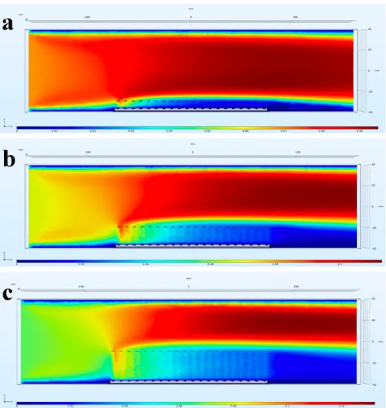
To evaluate the impact of height of structures on stationary flow profiles (using COMSOL), we compared each density of model at three heights, 1 cm, 2 cm, and 3 cm. All displayed similar patterns, so we will discuss the 10x20 cylindrical model. Figure 14 shows the velocity magnitude plots for the 10x20 models at 1 cm (Figure 14a), 2 cm (Figure 14b), and 3 cm (Figure 14c). The magnitudes were uniformly taken within a yz-plane in the center of the model, placing it halfway between two rows of cylinders, 0.25 cm away from each. The flow moves from left to right, and the legend below shows the relative change in velocity for each plot.
The plots show an increase in the magnitude of the velocity profile as the fluid progresses in the region above the model, with static flow speeds in the fluid region after the model. This is in contrast to the region within the model, which displays a rapid decrease in the velocity of the fluid as it passes through the cylinders. The tallest model retained the highest fluid velocity throughout the model, while the fluid within the smallest array slowed down quickly. In all three models there is a rapid change in velocity in the very beginning of the model, as the fluid initially interacts with the cylinders.
3.4.2 Variations in density
To compare the effects of varying density of arrays on resulting flow profiles, we compared the arrays of 2 cm in height of each density. In Figure 15, 15a shows the magnitude of velocity of the least dense 8x15 cylindrical model, 15b the 10x20 model, and 15c the densest 15x30 model. The magnitude was taken on a xy-plane at 1 cm of height in the model to display the change in the velocity profile as the fluid passes through the flow tank. The flow begins from the bottom of the plot at the initial velocity and drastically slows as it passes through the models. It is important to note here that the scales are relative to the plot, as some simulations reach a higher maximum velocity.
As seen in the figures, the least dense model allows the most steady flow to continue, with
Figure 15: Pseudocolor plots of the top view of the magnitude of the velocity profile in the COMSOL simulation representing the fluid flow over the varied density models at 2 cm of height. (a) shows the 8x15 cylinder model, (b) 10 x 20 cylinder, (c) 15 x 30 cylinder. Flow is from left to right, and the magnitude of the velocity for all three plots was taken on the xz-plane in the middle of the cylindrical array (z= -27.5). The range of velocity magnitude varied for each model and is depicted to the left of each plot.
Figure 15a displaying fluid velocity of up to 0.05 m/s in the middle of the array. In contrast, halfway through the medium dense model the maximum flow velocity is about 0.035 m/s and Figure 15c shows that the flow halfway through the densest model is nearly stagnant. It is also noticeable that the regions in the wakes of cylinders are immediately nearly stagnant, in contrast to the regions between cylinders with steady-streaming flow that persists for some time. As these stagnant areas interact with the fluid passing between cylinders, the average velocity of the system is slowed down until both regions are stagnant. These plots support our hypotheses as, based on Koehl’s research discussed in the introduction, the least dense model should allow the most flow to continue through it, while the denser models act more like solid objects redirecting fluid. It is very clear in comparing Figures 15a and 15c that the density of these models strongly affects how they redirect flow around them and create stagnant regions of fluid within the cylindrical structures.
4
Discussion
averages the velocity profile over time, the Brinkman model also averages over space, meaning that fluctuations in velocity profiles are generally smoothed out. While this is sufficient to model systems for some research, investigations into the detailed fluid dynamics found within macrophyte beds requires significant amounts of detail on the variations of flow and this amount of averaging may introduce significant error into the system when used to describe organisms responding to local flow conditions. For this reason, we require the continued development of more accurate models to better resolve the flow fields.
While both numerical methods produced good models of the flow fields, the IBAMR simula-tions produced temporally resolved flow fields and the generated time-varying vortical structures. These features were not captured by the stationary COMSOL simulations and therefore the IBAMR simulations contained significantly more detail. However, the solving of stationary models is much less computationally costly, and so depending on the research being performed and the computa-tional efficiency required, stationary simulations using COMSOL may be preferred to provide quick estimates of flow fields.
Increasing the height of the macrophyte array had various effects on the system. The height increased both the amount of steady flow remaining within the model and the amount of fluid being displaced, increasing the magnitude of the velocity in the fluid region above the model. In contrast, the small height of the smallest array created a very protected stagnant flow field within the cylinders, allowing nearly all the steady-streaming flow to continue uninterrupted through the system.
Variations in the density of these array also had a significant effect on the dynamics of the flow fields produced. The denser models not only allowed less flow into the array, they displaced the fluid in a way that is similar to solid structures, whereas the less dense models allowed fluid to filter through the cylinders. These results support Koehl’s findings on structures acting as solids of leaky sieves depending on the distance between them.[19]
4.1 Next steps
As mentioned in the introduction, these results are intended to bolster a larger project with the goal of creating accurate and detailed models of viscous and unsteady flows through complex and flexible structures and use these models to study the locomotion of planktonic organisms within macrophyte beds. The next steps in this project are threefold; the physical models of the macrophytes in this project use rigid cylinders, evenly spaced in a grid. By creating more flexible models of the vegetation, as well as arranging the components into more random and natural configurations, we will learn more about macrophytes interactions with environmental flows and the resulting intricate flow patterns that occur on small spatial scales.
Having obtained numerical simulations for the flow fields produced by the interaction between the fluid and these models which have been verified by experimental data, the project can use the quantified velocity profiles to augment our understanding of the locomotion of organisms in the aquatic environment. Future action in the project will include introducing these microorganisms into the controlled three-dimensional systems of flow for which we have these numerical models. Then, their behavior and movement will be studied, and the increased knowledge of the complex fluid dynamics of the system will be leveraged to denote patterns in behavior.
to gather fully-resolved flow fields of the environments. In reducing the amount of time required for simulations to produce steady-state data and increasing the complexities of the geometries this software can compute, the project would be improving the detail of the models as well as the options to study.
References
[1] G. C. Abade, B. Cichocki, M.L. E-Jezeska, G. Nagele, and E. Wajnryb. Short-time dynamics of permeable particles in concentrated suspensions. InJ. Chem. Phys., 2010.
[2] R.J. Adrian Particle–imaging techniques for experimental fluid mechanics. InAnn. Rev. Fluid Mech. 1991.
[3] Autodesk Fusion 360. https://www.autodesk.com/ [4] David Balmer. Separation of Boundary Layers. 2018.
[5] M.J. Berger, J. Oliger Adaptive mesh refinement for hyperbolic partial-differential equations. InJ. Comput. Phys. 1984.
[6] M.J. Berger, P. Colella Local adaptive mesh refinement for shock hydrodynamics. InJ. Comput. Phys. 1989.
[7] Bolt meshing software. https://www.csimsoft.com/boltoverview
[8] A. Cheer, S. Cheung, T. Hung, R.H. Piedrahita, S.L Sanderson Computational fluid dynamics of fish gill rakers during crossflow filtration. InBull. Math. Biol. 2012.
[9] A. DeBoer Computational fluid-structure interaction: Spatial coupling, coupling shell and mesh deformation. organs in air and water. Doctoral Thesis, 2008.
[10] B. Gaylord, D. Reed, L. Washburn, P. Raimondi Physical-biological coupling in spore dispersal of kelp forest macroalgae. InJ. Mar. Syst. 2004.
[11] B. E. Griffith. Hybrid finite difference/finite element version of the immersed boundary method. InInt. J. Numer. Meth. Engng., 2017.
[12] B.E. Griffith. An adaptive and distributed-memory parallel implementation of the immersed boundary (IB) method, 2014.
[13] D. Grunbaum, R.R. Strathmann Form, performance and trade-offs in swimming and stability of armed larvae. InJ. Mar. Res. 2004.
[14] Eike Hylla, O. Frederich, J. Mauß, F. Thiele. Application of the Immersed Boundary Method for the Simulation of Incompressible Flows in Complex and Moving Geometries. InNum. and Exp. Fluid Mech. 2010
[15] G. Jackson, C. Winant Effect of a kelp forest on coastal currents. organs in air and water. In
Cont. Shelf Res. 1983.
[16] Shannon K. Jones, Young J. J. Yun, Tyson L. Hedrick, Boyce E. Griffith, Laura A. Miller Bristles reduce the force required to ‘fling’ wings apart in the smallest insects. InJ. Exp. Biol. 2016.
[17] M.A.R. Koehl, M. Hadfield Hydrodynamics of larval settlement from a larva’s point of view. InIntegr. Comp. Biol. 2010.
[18] M. Koehl and Matthew A. Reidenbach Swimming by microscopic organisms in ambient water flow. InAnimal Locomotion, 2010.
[19] M Koehl. Transitions in function at lowRe: hair-bearing animal appendages. InMathematical Methods in the Applied Sciences, 2001.
[20] L. A. Levin Recent progress in understanding larval dispersal: New directions and digressions
[21] H. Masoud, H. A. Stone, and M. J. Shelley. On the rotation of porous ellipsoids in simple shear flows. InJ. Fluid Mech., 2013.
[22] R. McKibbin. Modeling pollen distribution by wind through a forest canopy. In JSME International Journal Series B, 2006.
[23] S. M. Mitran. Metachronal wave formation in a model of pulmonary cilia. InComput. Struct., 2007.
[24] G. Mo and A. S. Sangani. A method for computing Stokes flow interactions among spherical objects and its application to suspensions of drops and porous particles. Phys. Fluids, 1994. [25] D. Oliver and J. Chung. Flow about a fluid sphere at low to moderateRes. InJ. Fluid Mech.
1987.
[26] Eduard Marusic-Paloka1 and Andro Mikeli An Error Estimate for Correctors in the Homoge-nization of the Stokes and the Navier-Stokes Equations in a Porous Medium Boll. Unione Mat. Ital., 1996.
[27] C. S. Peskin. The immersed boundary method. InActa Numer, 2002.
[28] I. Proudman and J.R. Pearson. Expansions at smallRes for the flow past a sphere and a circular cylinder. InJ. Fluid Mech. 1957.
[29] M.A. Reidenbach, J.R. Koseff, M.A.R. Koehl Hydrodynamic forces on larvae affect their settlement oncoral reefs in turbulent, wave-driven flow. InLimnol. Oceanogr. 2009.
[30] U. Shavit, R. Rosenzweig, and S. Assouline. Free flow at the interface of porous surfaces: Generalization of the taylor brush configuration. InTransport in Porous Media, 2004.
[31] U. Shavit, R. Rosenzweig, G. Bar-Yosef, and S. Assouline. Modified brinkman equation for a free flow problem at the interface of porous surfaces: The cantor-taylor brush configuration case. InWater Resources Journal, 2002.
[32] C. Strickland, L. Miller, A. Santhanakrishnan, C. Hamlet, N. A. Battista, and V. Pasour. Three-dimensional lowReflows near biological filtering and protective layers. 14 Sep. 2017. [33] K. R. Sutherland Simultaneous field measurements of ostracod swimming behavior and
background flow. InASLO, 2011.
[34] L.D. Waldrop, L.A. Miller, S. Khatri A tale of two antennules: The performance of crab odour-capture. organs in air and water. InR. Soc. Interface, 2016.