Machine learning techniques for detection of glaucoma with optical coherence tomography angiography images

(1)

This document is downloaded from DR‑NTU (https://dr.ntu.edu.sg)

Nanyang Technological University, Singapore.

Machine learning techniques for detection of

glaucoma with optical coherence tomography

angiography images

Chan, Yam Meng 2020 Chan, Y. M. (2020). Machine learning techniques for detection of glaucoma with optical coherence tomography angiography images. Master's thesis, Nanyang Technological University, Singapore.

https://hdl.handle.net/10356/143892

https://doi.org/10.32657/10356/143892

This work is licensed under a Creative Commons Attribution‑NonCommercial 4.0 International License (CC BY‑NC 4.0). Downloaded on 13 Jan 2021 17:06:44 SGT

(2)

i

MACHINE LEARNING TECHNIQUES FOR DETECTION OF

GLAUCOMA WITH OPTICAL COHERENCE TOMOGRAPHY

ANGIOGRAPHY IMAGES

CHAN YAM MENG

SCHOOL OF MECHANICAL AND AEROSPACE ENGINEERING

(3)

ii

MACHINE LEARNING TECHNIQUES FOR DETECTION OF

GLAUCOMA WITH OPTICAL COHERENCE TOMOGRAPHY

ANGIOGRAPHY IMAGES

Submitted by:

Chan Yam Meng

School of Mechanical and Aerospace Engineering

Nanyang Technological University

A thesis presented to the

Nanyang Technological University

In partial fulfilment of the requirements for the

Degree of Master of Engineering

(4)

iii

Statement of Originality

I hereby certify that the work embodied in this thesis is the result of original research, is free of plagiarised materials, and has not been submitted for a higher degree to any other University or Institution.

13/05/2020

. . . . . . Date Chan Yam Meng

(5)

iv

Supervisor Declaration Statement

I have reviewed the content and presentation style of this thesis and declare it is free of plagiarism and of sufficient grammatical clarity to be examined. To the best of my knowledge, the research and writing are those of the candidate except as acknowledged in the Author Attribution Statement. I confirm that the investigations were conducted in accord with the ethics policies and integrity standards of Nanyang Technological University and that the research data are presented honestly and without prejudice.

15/5/2020 . . . . . .

(6)

v

Authorship Attribution Statement

This thesis contains material from 1 paper published in the following peer-reviewed journal in which I am listed as an author.

Chapter 3 (3.1, 3.2) and Chapter 4 (4.1, 4.2, 4.4.1) are published as Chan Yam Meng, E.Y.K. Ng, V Jahmunah, Joel En Wei Koh, Oh Shu Lih, Leonard Yip Wei Leon, U Rajendra Acharya, 2019, “Automated detection of glaucoma using Optical Coherence Tomography Angiography”, Computers in biology and medicine, Volume 115, 103483697-0814. https://doi.org/10.1016/j.compbiomed.2019.103483

The contributions of the co-authors are as follows:

• I wrote the manuscript with critical inputs from A/Prof Ng Yin Kwee and Dr U Rajendra Acharya.

• Dr Leonard Yip Wei Leon and I did data collection for the study.

• I implemented the model and performed data analysis with A/Prof Ng Yin Kwee, V Jahmunah, Joel En Wei Koh and Oh Shu Lih.

• All authors read and approved the final manuscript.

13/05/2020

. . . . . . Date Chan Yam Meng

(7)

vi

Abstract

Due to the ageing population in Singapore, chronic eye conditions which includes glaucoma, diabetic retinopathy, Aged Macular Degeneration (AMD) and cataract are estimated to rise significantly in numbers by year 2040.

Glaucoma is one of the most common causes of irreversible blindness and is the second most common cause of blindness worldwide, after cataracts. It usually goes

undetected until the disease progresses to a later or advanced stage. Therefore, this gives rise to a need for early detection of the disease to curb this issue before disease progression to an irreversible stage.

People above the age of 40 are usually advised to attend regular eye screenings for early detection of eye diseases. However, this is time-consuming for patients and taxing for practitioners who may be required to analyse many data and eye images within a fixed time frame. This may result in a deviation of diagnosis such as subjective prejudices over time due to fatigue. This report proposes to use machine learning techniques to detect glaucoma on optical coherence tomography angiography (OCTA) images.

To achieve this, two methods were proposed for the development of a Computer-aided Diagnosis (CAD) system. Both methods used adaptive histograms for image

pre-processing. The first method (Method 1) used the Local Phase Quantization (LPQ) for feature extraction, followed by feature selection using highly specific decision tree classifiers.

Finally, classification was done by using AdaBoost.

The second method (Method 2) used the Elongated Quinary Patterns (EQP) for feature extraction, followed by using statistical t-tests for feature selection. Highest

classification accuracy was achieved by using an ensemble classifier with the combination of Single-Layered Feedforward Neural Network (SFNN) and Logistic Regression model.

(8)

vii

The first method attained a diagnostic accuracy of 94.3% on optic disc-centred right eye images, whereas the second method attained a higher diagnostic accuracy of 95.1% on optic disc-centred left eye images.

The work done on this project has good potential in rapid screening of the eye for detection of glaucoma. Hence, it hopes to reduce the workload on practitioners in identifying patients with glaucoma using the method with high degree of accuracy and reliability.

(9)

viii

Acknowledgement

I would like to express my heartfelt gratitude towards my supervisor, A/Prof Eddie Ng Yin Kwee, for giving me the opportunity to work on this project. I am also grateful that he had shared his valuable experiences, given guidance and encouragement through this postgraduate journey.

I am very thankful to Adj Asst Prof Leonard Yip Wei Leon, Senior Consultant and Head of Glaucoma Services, from Tan Tock Seng Hospital for giving me permission to use his data and OCTA images in fulfilling the purpose of this project.

Finally, I would also like to thank Dr Rajendra Udyavara Acharya, Koh En Wei Joel, Oh Shu Lih Simon and Vicnesh Jahmunah from Ngee Ann Polytechnic for their great support and guidance towards the completion of the project.

The work presented in this report has been carried out at the School of Mechanical and Aerospace Engineering, Nanyang Technological University (NTU).

(10)

ix

3.2.2 Contrast Limited Adaptive Histogram Equalization (CLAHE) 27 3.2.3 Feature Extraction using Local Phase Quantization (LPQ) 28 3.2.4 Validation using k-fold Cross Validation and z-score Normalization 30 3.2.5 Feature Selection using Decision Tree 31 3.2.6 Classification using AdaBoost 32 3.3 Methodology based on Elongated Quinary Pattern feature extraction (Method 2) 33

3.3.1 Image pre-processing 34

3.3.2 Feature Extraction using Elongated Quinary Patterns (EQP) 34 3.3.3 Gray-Level Co-occurrence Matrix (GLCM) 35 3.3.4 Gray-Level Run Length Matrix (GLRLM) 36

3.3.5 Entropies 37

3.3.6 Feature Selection using t-test 40

3.3.7 Classification Models 40

3.3.7.1 Single-Layered Neural Network (SLNN) 40 3.3.7.2 Support Vector Machine (SVM) 41 3.3.7.3 Logistic Regression Model 42 3.3.8 Validation using 10-fold Cross Validation, z-score and ADASYN 43 Chapter FOUR – Results and Discussion 44

4.1 Results 44

4.2 Results (Method 1) 46 4.2.1 Classification Outcomes (Method 1) 46

(12)

xi

4.3.1 Classification Outcomes (Method 2) 54

4.4 Discussion 58

4.4.1 Selected CAD studies for automatic detection of Glaucoma 58 4.4.2 Discussion of Work done in the Thesis 60 Chapter FIVE – Conclusion and Future Works 64

5.1 Conclusion 64

5.2 Future Work 66

References 67

(13)

xii

List of Figures

Figure 1: Patient undergoing HVF testing 1 Figure 2: Anatomy of the human eye 2 Figure 3: Schematic diagram Primary Angle Closure Glaucoma 4 Figure 4: Schematic diagram Primary Open Angle Glaucoma 6 Figure 5: GAT IOP measurement on a patient’s eye 9 Figure 6: HVF 24-2 SITA Visual Field test results chart 10 Figure 7: Clinician performing slit lamp examination on a patient 11 Figure 8: Performing Gonioscopy on the eye 12 Figure 9: Anatomy of (a) normal optic disc and (b) optic disc with glaucoma damage 14 Figure 10: Optic disc captured by HRT (a) normal optic disc 15

(b) optic disc with “cupping”

Figure 11: Comparison of a normal vs glaucoma on OCT 17 Figure 12: OCTA disc images of non-glaucoma patients 19 Figure 13: OCTA macula images of non-glaucoma patients 20 Figure 14: OCTA disc images of glaucoma patients 21 Figure 15: OCTA macula images of glaucoma patients 22 Figure 16: Segmentation layers within OCTA macula images 24 Figure 17: Flow diagram of the Method 1 to detect glaucoma on OCTA images 24 Figure 18: Flow diagram of image pre-processing steps 27 Figure 19: Function of LPQ feature extraction algorithm 29 Figure 20: k-fold Cross-validation on 5-fold iteration training model 31 Figure 21: Flow diagram of Method 2 to detect glaucoma on OCTA images 33 Figure 22: EQP encoding based on 5 values 35

(14)

xiii

Figure 23: Single-Layered Neural Network 41 Figure 24: Obtaining the Optimal hyperplane using SVM 42 Figure 25: Bar graph of 5-fold Hu’s Moment on OD Disc 47 Figure 26: Bar graph of 5-fold Hu’s Moment on OS Disc 47 Figure 27: Bar graph of 10-fold Hu’s Moment on OD Disc 48 Figure 28: Bar graph of 10-fold Hu’s Moment on OS Disc 48 Figure 29: Bar graph of 5-fold LPQ on OD Disc 49 Figure 30: Bar graph of 5-fold LPQ on OS Disc 50 Figure 31: Bar graph of 10-fold LPQ on OD Disc 50 Figure 32: Bar graph of 10-fold LPQ on OS Disc 51 Figure 33: Comparison of Classification Outcomes (LPQ vs Hu’s Moment) 52 Figure 34: Comparison of Classification Outcomes (5-fold vs 10-fold LPQ) 53 Figure 35: Comparison of standalone classifiers on OD Disc images 54 Figure 36: Comparison of standalone classifiers on OS Disc images 55 Figure 37: Comparison of standalone classifiers on OD Macular images 55 Figure 38: Comparison of standalone classifiers on OS Macular images 56 Figure 39: Comparison of Standalone Classifier vs Ensemble Classifier 57

(15)

xiv

List of Tables

Table 1: Classification of retinal layers on OCTA images 23 Table 2: Variables defined for use on SFNN model in project 41 Table 3: Summary of work presented in this report 45 Table 4: Types of Variables used in presentation of results 46 Table 5: Best results from different methods using Hu Moment 49 Table 6: Best results from different methods using LPQ 51 Table 7: Best Classification Outcomes comparison (Hu’s Moment vs LPQ) 52 Table 8: Best Classification Outcomes comparison (5-fold vs 10-fold LPQ) 53 Table 9: Overall classification outcomes based on standalone classifiers 56 Table 10: Overall classification outcomes based on the ensemble classifier 57 Table 11: Best Classification Outcomes comparison (SFNN vs SFNN+LogReg) 57 Table 12: Best Classification Outcomes comparison (Method 1 vs Method 2) 60 Table 13: Pros and Cons of Method 1 vs Method 2 61

(16)

xv

List of Appendices

Appendix A1: Results based on Hu’s Moment Feature Extraction on OD Disc 77 Table A1a: Hu Moment with Addition on 5-fold cross validation (OD Disc) 77 Table A1b: Hu Moment with Multiplication on 5-fold cross validation (OD Disc) 78 Table A1c: Hu Moment with PCA on 5-fold cross validation (OD Disc) 79 Table A1d: Hu Moment with Addition on 10-fold cross validation (OD Disc) 80 Table A1e: Hu Moment with Multiplication on 10-fold cross validation (OD Disc) 81 Table A1f: Hu Moment with PCA on 10-fold cross validation (OD Disc) 82

Appendix A2: Results based on Hu’s Moment Feature Extraction on OS Disc 83 Table A2a: Hu Moment with Addition on 5-fold cross validation (OS Disc) 83 Table A2b: Hu Moment with Multiplication on 5-fold cross validation (OS Disc) 84 Table A2c: Hu Moment with PCA on 5-fold cross validation (OS Disc) 85 Table A2d: Hu Moment with Addition on 10-fold cross validation (OS Disc) 86 Table A2e: Hu Moment with Multiplication on 10-fold cross validation (OS Disc) 87 Table A2f: Hu Moment with PCA on 10-fold cross validation (OS Disc) 88

Appendix B1: Results based on LPQ Feature Extraction on OD Disc 89 Table B1a: LPQ with Addition on 5-fold cross validation (OD Disc) 89 Table B1b: LPQ with Multiplication on 5-fold cross validation (OD Disc) 90 Table B1c: LPQ with PCA on 5-fold cross validation (OD Disc) 91 Table B1d: LPQ with Addition on 10-fold cross validation (OD Disc) 92 Table B1e: LPQ with Multiplication on 10-fold cross validation (OD Disc) 93 Table B1f: LPQ with PCA on 10-fold cross validation (OD Disc) 94

Appendix B2: Results based on LPQ Feature Extraction on OS Disc 95 Table B2a: LPQ with Addition on 5-fold cross validation (OS Disc) 95 Table B2b: LPQ with Multiplication on 5-fold cross validation (OS Disc) 96 Table B2c: LPQ with PCA on 5-fold cross validation (OS Disc) 97 Table B2d: LPQ with Addition on 10-fold cross validation (OS Disc) 98

(17)

xvi

Table B2e: LPQ with Multiplication on 10-fold cross validation (OS Disc) 99 Table B2f: LPQ with PCA on 10-fold cross validation (OS Disc) 100

Appendix C: Summary of CAD systems using OCTA for the diagnosis of glaucoma 101

(18)

1

CHAPTER ONE – Introduction

Glaucoma is one of the most common causes of irreversible blindness in the world (Antonio et al, 2016). It affects the peripheral vision, which is the surrounding vision or side vision. Glaucoma is usually termed as the “Silent thief of sight”, as patients do not experience any pain or realize they have lost vision (Wiggs and Weinreb, 2014). It usually goes undetected until the disease progresses to a later or advanced stage.

Nowadays, there are various methods available to diagnose glaucoma. In current clinical practice, doctors will be able to diagnose glaucoma by measuring the patient’s intra-ocular pressure (IOP) and by evaluating the visual field losses within the eye using Humphrey visual field (HVF) test (Figure 1) (Kahook et al, 2007).

Figure 1: Patient undergoing HVF testing

Source: Glaucoma Research Foundation, Why Do I need a Visual Field test?

Extracted from: https://www.glaucoma.org/treatment/why-do-i-need-a-visual-field-test.php

Date accessed: 27 May 2019

Other methods involve the use of various imaging modalities to detect the presence of optic nerve damage and cup disc changes. These imaging modalities are discussed in the next chapter (Chapter 2).

(19)

2

This project aims to automate the detection of glaucoma using machine learning techniques with optical coherence tomography angiography (OCTA) images. The development of accurate, fast, and robust automated system can help to reduce the burden on clinicians.

1.1 The Human Eye

The human eye is one of the most important and complex organs in the human body (Colin et al, 2010). The eye is made up of 3 different layers (Figure 2).

Figure 2: Anatomy of the human eye

Source: ThoughtCo. Structure and Function of the Human Eye

Extracted from: https://www.thoughtco.com/how-the-human-eye-works-4155646

The outermost layer comprises of the cornea and the sclera. The sclera is a thick white layer which covers the eyeball, whereas the cornea is a transparent, convex window at the

(20)

3

front of the eye which allows light to pass through it easily (Shyamanga et al, 2012). Any breaks in the cornea will result in pain or irritation.

The middle layer is made up of iris, lens and choroid (Colin et al, 2010). The pupil is present within the iris, which controls the size of it. Controlling the size of the pupil controls the amount of light entering the retina. The crystalline lens is made up of multi-layered and a specific arrangement of lens fibrils. Fibres from the ciliary body that controls the shape of the lens are attached to nuclear region surrounded by soft cortex region (Shyamanga et al, 2012). The choroid is a vascular layer that carries nutrients and oxygen to outer retinal layers (Colin et al, 2010).

The inner layer of the eye comprises of the retina, which is a thin neurovascular layer containing lot of specialised cells that capture and process light (Shyamanga et al, 2012). Cones and rods are the two types of photoreceptors that are located on the outermost part of the retina. Rods are sensitive to dim light vision and cones are sensitive to colour vision in bright illumination (Shyamanga et al, 2012). The retina nerve fibre layer is formed by unmyelinated axons of the ganglion cells. These axons are wired towards the optic disc, where they leave the eye through an opening in the sclera to form the optic nerve (Shyamanga et al, 2012). The most sensitive portion of the retina, which contains the highest number of cones, is the macula region. The most sensitive portion of the macula is called the fovea (Shyamanga et al, 2012).

1.2 Glaucoma

Glaucoma is the second most common cause of blindness worldwide, after cataracts (Antonio et al, 2016). It presents a great health concern as it is usually undetectable during the early stages without regular screening. Visible symptoms of glaucoma may only appear at a later stage. It affects peripheral vision and may progress over time without treatment. It leads to irreversible blindness, unlike cataract.

(21)

4

Glaucoma belong to a group of neuropathies characterized by the degeneration of retina ganglion cells resulting in changes to the optic nerve head (Robert N et al, 2014). The reduction in ganglion cells, which causes morphological changes in the retina, leads to cupping of the optic nerve head. As a result of cupping, the optic nerve head loses axons due to chronic glaucoma (Antonio et al, 2016). There are two main types of glaucoma, namely, primary angle closure glaucoma and primary open angle glaucoma.

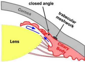
1.2.1 Primary Angle Closure Glaucoma (PACG)

The occurrence of the primary angle closure glaucoma (PACG) presents an emergency. This is due to the mechanical closure of the aqueous drainage angle (Figure 3), which is different from primary open angle glaucoma. The risk of primary angle closure glaucoma increases with age.

Figure 3: Schematic diagram Primary Angle Closure Glaucoma

Source: Stepwards, Open-angle Glaucoma Extracted from: https://www.stepwards.com/?page_id=6617

(22)

5

There are two causes for primary angle closure glaucoma. The first cause is the blockage of the pupillary. Fibres settled down over time inside the lens, result in the thickening of the lens. This phenomenon pushes the structure forward, eventually touching the iris, which is positioned in front of it. This causes resistance to the flow of fluid from the ciliary body through the pupil. When the resistance becomes too high and it blocks fluid from passing through the pupil, a pupil block occurs and causes the iris to be pushed forward, occluding the trabecular meshwork (Shyamanga et al, 2012). The high pressure formed due to this resistance and pupil block affects blood supply to the optic nerve, which results in optic nerve damage with corresponding visual field defects.

The second cause of primary angle closure glaucoma is the plateau iris. It is due to anatomic variation at the positioning of the root of the iris and is more prevalent in younger patients. The positioning causes the blockage of the drainage angle, which leads to angle closure glaucoma.

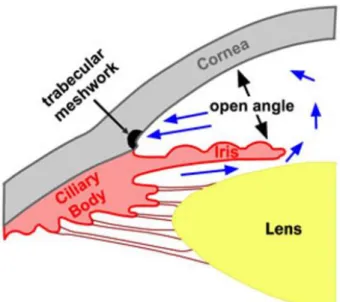
1.2.2 Primary Open Angle Glaucoma (POAG)

The primary open angle glaucoma (POAG) encompasses the open angle glaucoma (OAG) and the ocular hypertension (OHT), in which both types of glaucoma experience the increase in ocular pressure within the eye. The normal tension glaucoma (NTG), which is also a type of primary open angle glaucoma (POAG), will have no measured increase in the intraocular pressure (Figure 4) (Shyamanga et al, 2012). The onset of primary open angle glaucoma is different from that of the primary angle closure glaucoma. Field defect develops over a long period of time which requires long-term monitoring.

(23)

6

Figure 4: Schematic diagram Primary Open Angle Glaucoma

Source: Stepwards, Open-angle Glaucoma Extracted from: https://www.stepwards.com/?page_id=6617

Open angle glaucoma usually does not show symptoms until later stages when the loss of vision is no longer reversible or can be treated. This results in the loss of peripheral (surroundings) vision which cause patients to not notice things or objects coming from their side, resulting in bumping into things unknowingly. Elevated intra-ocular pressure (IOP) without any visual field loss or defects are termed as ocular hypertension.

1.3 Research Hypothesis

The main hypothesis of this research is that the application of machine learning algorithms can automate, differentiate and detect glaucoma patients using Optical Coherence Tomography Angiography (OCTA) images with a high degree of accuracy. Based on this hypothesis, the main objective derived for this project is to achieve at least 90% detection accuracy.

(24)

7

CHAPTER TWO – Literature Review

There are various methods to diagnose the presence of glaucoma in patients. Four common methods to clinically diagnose glaucoma are discussed in this chapter. Regular eye examinations are required to diagnose glaucoma at its early stages, especially for primary open angle glaucoma, which are asymptomatic until later stages of the disease.

With the advancement of imaging technology, various imaging modalities can also be used to help the clinicians in identifying the presence of glaucoma and glaucomatous changes within a patient’s eye. Most of the imaging modalities are inexpensive and non-invasive methods. These different modalities are discussed in the chapter.

Image processing is always been a major area of research over the years. With better technology and computing tools these days, one can quantify and visualize abnormalities within the eye accurately. The advantages of the non-invasiveness of image acquisition through the different imaging modalities and platforms present researchers an opportunity to develop advanced computer-aided diagnosis (CAD) systems for the detection of eye abnormalities.

The various steps involved in the development of typical CAD system are (i) image pre-processing, (ii) image transformation, (iii) feature extraction, (iv) feature selection and (v) classification. Adaptive histograms were utilized for image pre-processing, which was followed by using feature extraction methods such as the Local Phase Quantization (LPQ), Hu’s Moment and Elongated Quinary Patterns (EQP). Feature selection was done by using statistical t-tests and decision tree classifiers. Finally, classification were done by using AdaBoost, a type of ensemble classifier, which combines multiple classifiers into a composite model to achieve better accuracy and results as well as different standalone classifiers such as Single Layered Neural Network (SLNN), Support Vector Machine (SVM) and Logistic Regression Models.

(25)

8 2.1 Tests used for the detection of glaucoma

There are 4 common tests employed by clinicians to diagnose glaucoma in clinical settings are given below:

• measurement of IOP using tonometer,

• checking for visual field losses and defects with perimetry instrument. Humphrey visual field (HVF) is commonly used tests for visual field defects.

• examination of optic nerve damage via opthalmoscopy.

• differentiating whether it is closed or open angle glaucoma using gonioscopy.

2.1.1 IOP measurement using tonometry

The measurement of IOP plays an important role especially in the detection of primary open or closed angle glaucoma. Under clinical settings, the current gold standard used is Goldmann applanation tonometry (GAT). Local anaesthetic drops will be applied onto the patient’s eye prior to examination. Clinicians will use a prism device, with a blue filter on the slit lamp to contact and indent the apex of the cornea. They will then adjust the applanation tonometry rings using a dial on the side of the slit lamp such that the edges of the rings meet, then measurement will be taken (Figure 5) (Stevens et al, 2007).

(26)

9

Figure 5: GAT IOP measurement on a patient’s eye

Source: verywellhealth, How Tonometry Eye Pressure Test Works

Extracted from:https://www.verywellhealth.com/tonometry-eye-pressure-test-3421842

Date accessed: 28 May 2019

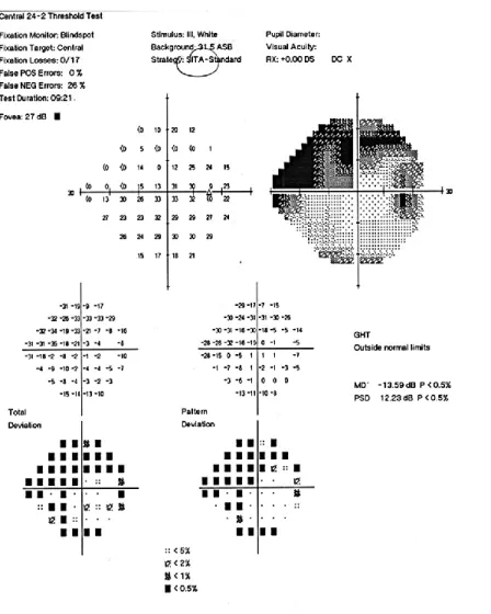
2.1.2 Humphrey visual field testing (HVF)

HVF testing aids clinicians to detect and monitor the progression of glaucoma. The visual field test maps out the area of vision and show the changes in the field of vision of the patient’s eye (Kahook et al, 2007). The patient will be seated in front of the machine, and rest on the chin rest. Appropriate lenses or glass correction will be inserted on the machine if needed. The patient will then be required to fixate their gaze onto the fixation light in the centre and click the button given whenever he/she observes flickering lights coming from the side. The results chart of HVF 24-2 SITA is shown on Figure 6.

(27)

10

Figure 6: HVF 24-2 SITA Visual Field test results chart

Source: University of Iowa Healthcare, Hypotony: Late hypotony from trabeculectomy and Ahmed seton with resulting hypotony maculopathy

Extracted from: https://webeye.ophth.uiowa.edu/eyeforum/cases/250-hypotony.htm

There are various factors taken into consideration when the results are being interpreted by the practitioner. Indicators such as false positives and negatives could help to indicate if the patient had fixated their eye on the centre target or not. Clinicians will also observe the numbers presented on the chart on the numeric results graph (in decibels, dB). If the value presented is

(28)

11

above 40 dB, this may indicate that the patient has been over-clicking on the device causing results to be inaccurate and not reliable (Kahook et al, 2007).

Dark shaded areas at the peripheral of the retina presented in the chart shows signs of visual losses (Figure 6). Readings such as the mean deviation (MD) and pattern standard deviation (PSD) may indicate signs of glaucoma and localized visual losses respectively (Kahook et al, 2007).

2.1.3 Ophthalmoscopy

Ophthalmoscopy, also known as funduscopy, is a test which allows clinician to view inside the eye, known as fundus, using an ophthalmoscope or a slit lamp instrument with condensing lens (Figure 7). It is usually included as a part of routine examination. Patients’ eyes will be usually dilated with local dilation drops (Tropicamide) prior to examination.

Figure 7: Clinician performing slit lamp examination on a patient

Source: Tan Tock Seng Hospital, Glaucoma brochure

Clinicians can use ophthalmoscopy to examine the optic cup disc for glaucoma signs within the eye, such as; the optic disc size, colour and cup-to-disc ratio if they exceed the normal threshold (David, 2004). The optic nerve head can also be visible during opthalmoscopy.

(29)

12 2.1.4 Gonioscopy

The gonioscopy is used for different purposes as compared to the first 3 methods. It examines the drainage angle (Shyamanga 2012) of the eye to determine if the patient has open or closed angle glaucoma (Figure 8). A closed angle will usually cause a sudden and rapid surge in IOP which is an acute form of glaucoma. Gonioscopy can also be used to examine the abnormality in blood vessels or damage from any history of eye trauma (Bollinger et al, 2017).

Figure 8: Performing Gonioscopy on the eye

Source: Health Education Library for People (HELP)

Extracted from: http://www.healthlibrary.com/

(30)

13

2.2 Types of imaging modalities used for the detection of glaucoma

This section will examine the various imaging modalities which can be used to diagnose glaucoma. The modalities covered include fundus photography, Heidelberg retina tomography (HRT), optical coherence tomography (OCT) and optical coherence tomography angiography (OCTA).

2.2.1 Fundus/Optic Nerve Photography for Glaucoma

The history of fundus photography traces back to as far as in the 1860s (Myers et al, 2018). The examination of optic nerve had always been a crucial clue to whether the patient has glaucoma. With the use of colour fundus photos, clinicians can determine and diagnose glaucoma based on the cup-to-disc ratio on the optic disc.

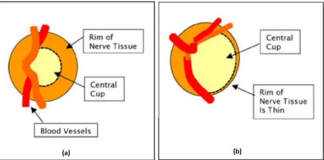
One of the glaucomatous changes that can be observed on the optic disc is the change in colour and its appearance. A normal optic disc usually presents a pinkish and orange colour, with a pale centre, where the cup is located. Due to glaucoma, the colour of the optic disc fades and appears pale as a whole (Figure 9). An increase in the cup size will signify the possible presence of glaucoma.

(31)

14

Figure 9: Anatomy of (a) normal optic disc and (b) optic disc with glaucoma damage

Source: Craig Blackwell MD, Testing for Glaucoma

Extracted from: http://www.blackwelleyesight.com/narrated-eye-exam/testing-for-glaucoma/

Several studies have reported in their literature that optic disc is the main structure for the detection of glaucoma disease. Image segmentation methods involving multi-thresholding and active contour method were used to mark out the boundaries of the optic disc and cup, in which the ratio is subsequently computed based on the area of cup to the optic disc (Mishra et al, 2011).

2.2.2 Heidelberg Retinal Tomography (HRT)

The Heidelberg retinal tomography (HRT) utilizes a special laser to obtain 3D photographs of the optic nerve and its surrounding tissues to make an accurate observation of the optic nerve head, which cannot be done on a normal clinical examination. The HRT enables the computation of optic disc area, volume of the cup and the area of the rim around the cup. The HRT can continuously take images below the surface of the optic nerve in layers until the

(32)

15

required depth. After capturing these images, the machine will combine them together to form a 3-dimensional image of the optic nerve.

“Cupping” occurs when there is optic nerve damage due to glaucoma. The abnormal indent on the optic nerve head can show signs of nerve damage, which will be picked up and measured by HRT (Figure 10).

Figure 10: Optic disc captured by HRT (a) normal optic disc (b) optic disc with “cupping”

Source: Maslin JS, Mansouri K, Dorairaj SK, “HRT for the Diagnosis and Detection of Glaucoma Progression”, 2015, Open Ophthalmol J, 15;9:58-67

Older models of the HRT were mainly used for research purpose and is highly operator reliant and not easy to use (Maslin et al, 2015). The latest model of the HRT, HRT III, provides analysis of the optic disc without the need for manual line placement, hence eliminating the need of an operator (Maslin et al, 2015). The automation increases the reproducibility and reliability of measurements obtained. The machine has its own database of patients from different descent to aid in the automated detection of the optic nerve head and disc.

(33)

16

2.2.3 Optical Coherence Tomography (OCT) for Glaucoma

OCT is a commonly used imaging modality used to determine and evaluate structural damage in the eye due to glaucoma. It provides a 3-dimensional cross-section imaging of the optic nerve head and the retina. Currently the most commonly used method for glaucoma assessment is the spectral domain (SD) OCT. The SD-OCT has higher scanning speeds, which means its less prone to inaccuracies and artefacts due to eye movements (Bussel et al, 2013).

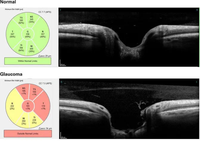
Similar to that of the HRT, 3-dimensional OCT images allows accurate measurements of the optic disc, rim area, cup to disc ratio and cup volumes. Unique quality to OCT is its ability to measure the retinal nerve fibre layer (RNFL) thickness for diagnosis of glaucoma. The measurement of the RNFL thickness enables clinicians to differentiate between normal eyes and eyes with advanced glaucoma damage (Bussel et al, 2013). However, due to slight or even subtle changes to the RNFL thickness in early stages of glaucoma, the differences may not be significant enough to be picked up by OCT based on thickness measurement (Bussel et al, 2013). Measuring of RNFL thickness can also help clinicians to monitor the progression of glaucoma in identified patients (Figure 11).

(34)

17

Figure 11: Comparison of a normal vs glaucoma on OCT

Source: Heidelberg Engineering, What is an OCT examination?

Extracted from: https://know-the-eye.heidelbergengineering.com/eye-disorders/glaucoma/

The RNFL thickness, together with different areas and segments of optic nerve head, presents an important focal point in the development of machine learning or deep learning algorithms for the detection of glaucoma. Feature extraction algorithms were used to map out the thickness and deviations data, while transfer learning on convolutional neural networks (CNN) was employed for features such as disc and macular RNFL thickness maps and the disc and macular ganglion cell complex (GCC) thickness maps (An et al, 2019). The machine learning system is used to distinguish healthy subjects from subjects with glaucoma accurately using set of parameters listed (An et al, 2019).

(35)

18

2.2.4 Optical Coherence Tomography Angiography (OCTA) for Glaucoma

OCTA is relatively a new ocular imaging modality. It provides a high-resolution image of the vessels and blood flow within the retina and the optic nerve head. The current OCTA does not require injection of dye into the patient, is non-invasive and able to produce results fast (Simon et al, 2016).

A major advantage of using the OCTA is that most SD-OCT devices already have the software and hardware required and need the software. OCTA uses similar recording properties as the structural OCT as well as the require light source (Daneshvar et al, 2017). Furthermore, OCTA allows capturing of images of the various retinal layers such as; the superficial layer, outer retinal layer, deep layer and the choroidal layer with good reproducibility and repeatability. This enables visualization of structural changes caused due to glaucoma on each individual layers of the retina. OCTA images that were used in analysis for this study is shown from Figure 12 to Figure 15.

A major drawback of the OCTA at the current scanning speed makes it susceptible to various artefacts, such as motion caused by patient movement, shadow from vessels and patient blinking (Daneshvar et al, 2017). OCTA has limited field of view, but this can be easily countered by stitching multiple OCTA images of different fields together.

It is shown in various studies that glaucomatous changes in patients will cause reduction in blood flow, vascular density, and vessel size in their retina, as compared to healthy subjects (Lee et al, 2016). Such evidence proved that OCTA can be useful in the diagnosis of glaucoma. Other imaging modalities used in the past such as indocyanine green angiography (ICGA) and retinal fluorescein, require a dye, or a contrast medium to be injected to the patient’s eye (Simon et al, 2016). Their images are acquired over a set period of time. OCTA provides a rapid yet

(36)

19

non-invasive method to measure the similar set of parameters as the other modalities (Daneshvar et al, 2017).

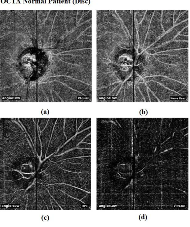
Figure 12: OCTA disc images of non-glaucoma patients

(a) Choroid (b) Nerve head (c) Radial Peripapillary Capillaries (RPC) (d) Vitreous

Source: Cross-sectional Prospective Observational Cohort study conducted by the Department of Ophthalmology, Tan Tock Seng Hospital, Singapore

(37)

20

Figure 13: OCTA macula images of non-glaucoma patients

(a) Choroid capillary (b) Deep (c) Outer Retina (d) Superficial

(38)

21

Figure 14: OCTA disc images of glaucoma patients

(a) Choroid (b) Nerve head (c) RPC (d) Vitreous

(39)

22

Figure 15: OCTA macula images of glaucoma patients

(a) Choroid capillary (b) Deep (c) Outer Retina (d) Superficial

(40)

23

CHAPTER THREE – Methodology

3.1 Data Used

The OCTA images were obtained and used with permission from the Department of Ophthalmology, Tan Tock Seng Hospital (TTSH), Singapore. Approval was granted by the NHG Domain Specific Review Board (DSRB) (NHG DSRB Ref: 2019/00138) for the usage of images in this study.

These images had been captured using the AngioVue Enhanced Microvascular Imaging System from Optovue. This system was used to capture both the optic nerve head and macular images per patient visit. There were 89 non-glaucoma patients with 1228 optic nerve head (disc) images and 632 macular images, and 46 glaucoma patients with 420 optic nerve head (disc) images and 364 macular images used for this project. All OCTA images have a resolution of 304 x 304 pixels and are captured in PNG format.

The images are further classified into different retinal layers as shown in Table 1:

Disc Macula Choroid Disc Choroid Retina Nerve head Deep

RPC Outer Retina

Vitreous Superficial

Table 1: Classification of retinal segmentation layers on OCTA images

This project aims to automate the detection of glaucoma on OCTA images using machine learning techniques with a minimum of 90% accuracy. The algorithm will be packaged into a usable software for clinicians’ use during their clinic sessions. The research hypothesis is that the automated detection can achieve at least 90% accuracy on both optic disc and macular OCTA images.

(41)

24

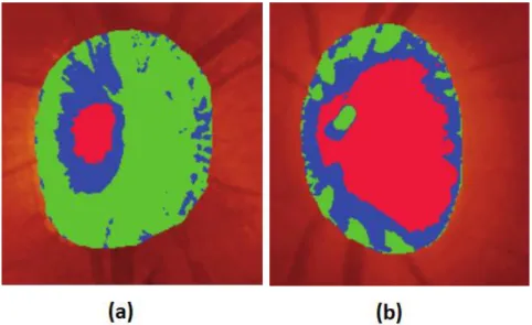
Figure 16 illustrates the location of 4 different segmentation layers: (a) Superficial layer, (b) deep layer, (c) outer retina layer, (d) choroid capillaries layer, within OCTA macular images.

Figure 16: Segmentation layers within OCTA macula images

Source: Yam Meng Chan, EYK Ng, V Jahmunah, Joel En Wei Koh, Oh Shu Lih, Leonard Yip Wei Leon, U Rajendra Acharya, “Automated detection of glaucoma using Optical Coherence

Tomography Angiogram images”, 2019, Computers in Biology and Medicine 3.2 Methodology based on Local Phase Quantization feature extraction (Method 1)

Figure 17: Flow diagram of Method 1 to detect glaucoma on OCTA images

Figure 17 shows the overview of the processes involved in the first proposed method to detect glaucoma on OCTA images.

Preprocessing of eye images Feature extraction using LPQ Data fusion/ PCA 10-fold cross validation, z-score normalization Feature selection using Decision Tree Classification using AdaBoost

(42)

25

Image pre-processing was performed to resize the OCTA images, followed by

converting them to grayscale. Adaptive histogram (Zhu and Huang, 2012) was then employed to improve the contrast on the images.

Features were then extracted from the images using Local Phase Quantization (LPQ) (Ojansivu and Heikkila, 2008), an image analysis method based on the blur invariance property of the Fourier phase spectrum (Ojala et al, 2002), calculated in local image

windows. LPQ serves as a texture classification method that is insensitive to blurring caused by motion or atmospheric turbulence. In this study, LPQ is calculated locally at each

pixelated region, generating histograms.

Features extraction using Hu’s moment invariants were employed to compare the accuracy of results against the LPQ method. Image moments are made up of averages of different pixel intensity weights (Mallack 2018). Hu moment invariants are made up of a set of 7 numbers invariant to image transformation. They are calculated using central moments which are mainly invariant to scale, rotation, translation, and reflection (Mallack 2018). The LPQ method was able to extract 256 features, as compared to only 7 from the Hu’s moment method, was chosen for use in the proposed method.

Subsequently, data fusion techniques (Castanedo, 2013); which includes the Addition, Multiplication and PCA methods, were used to aggregate the data into more actionable data for efficient analysis. Addition, followed by multiplication were explored whereby the extracted features were added and multiplied respectively. Principal component analysis (PCA) (Jolliffe, 2002) was then employed, to reduce the dimensionality of a large dataset such that it constitutes smaller data, while retaining most of the variations amongst the data. PCA works by rotating the data amplifying the variance in the new axes, thus projecting high-dimensional data into a low dimensional space (Indhumathi and Sathiyabama, 2010). PCA was chosen in

(43)

26

the end as the data fusion technique used in this report as it yields the highest accuracies and performances on the dataset.

10-fold cross validation (Vicnesh and Hagiwara, 2019) was then employed to evaluate the proposed method, whereby ten iterations were conducted to obtain the average

performances in terms of accuracy, sensitivity, specificity, and positive predictive value. Z-score normalization (Gopal et al, 2015) was then applied, such that the original unstructured data is presented within a structured range.

Highly significant features were then selected using Decision Tree classifier (Vicnesh and Hagiwara, 2019) using predictor importance. This empowers the training model to predict the classification accurately.

Classification was then done with AdaBoost algorithm (Freund, 1995) (Kim and Upneja, 2014). This is a self-adjustable algorithm that works by generating a set of various classifiers to improve the performance of weak classifiers. It automatically adjusts to the error rate of the algorithm to modify the probability distribution of each sample. A larger weight is set for wrongly classified sample and vice versa, enabling a strong classifier to be generated.

The parameters accuracy, sensitivity, specificity, and precision were used for evaluation.

3.2.1 Image pre-processing

Prior to feature selection and analysis of the data, image pre-processing was

performed to ensure all data are normalized to each other before actual analysis. Three pre-processing steps were employed to achieve image normalization. The OCTA images are first resized to 300 x 300 pixels, then they were all converted to grayscale and lastly a Contrast Limited Adaptive Histogram Equalization (CLAHE) is applied. The image pre-processing steps are outlined in Figure 18.

(44)

27

Figure 18: Flow diagram of image pre-processing steps

3.2.2 Contrast Limited Adaptive Histogram Equalization (CLAHE)

Due to the susceptibility of OCTA images to artefacts and noise (as described in Section 2.2.4), resulting in poor contrast, contrast enhancement techniques such as the CLAHE is employed to improve image quality. Contrast enhancement improves the differences between the image intensities of pixels within close distance (Singh and Patel, 2017). The speed of determining and identifying diseases on the OCTA depends on how efficient the contrast enhancement is (Singh and Patel, 2017).

Histogram equalization has been credited for being simple and efficient. The histogram adjusts the gray level of an image according to the distribution of probability and stretches the range of the distribution to enhance the contrast and visual effects of it (Zhu and Huang, 2012).

The CLAHE specifically targets entropy of an image and achieves best equalization using the maximum entropy (Pizer et al, 1987). Contrast limited as its name suggests, it eliminates a common issue of an ordinary Adaptive Histogram equalization (AHE) to overamplify near-consistent regions within an image as the histogram of such regions are usually dense and highly concentrated. CLAHE allows the user to set a predefined value in which to restrict and limit the contrast amplification to reduce such issue encountered using a normal AHE (Pizer et al, 1987).

(45)

28

3.2.3 Feature Extraction using Local Phase Quantization (LPQ)

Features were extracted from the images using local phase quantization (LPQ) (Ojansivu and Heikkila, 2008), an analysis technique based on the blur invariance aspect of the Fourier phase spectrum (Ojala et al, 2002) calculated in local image windows. In digital image processing, the distinct model for spatially shift-invariant blurring of an image f(x,y) ensuing in an observed image g(x,y) can be expressedas the equation (1) as shown below:

g(x,y) = f(x,y) * h(x,y) + n(x,y),

(1) where h(x,y) is defined as the point spread function (psf) of the model, n(x,y) as noise and * as 2D convolution. The LPQ features use the local phase information that is extracted by the 2D discrete Fourier transforms, computed over a rectangular area denoted as 𝑁(𝑥, 𝑦)and only four frequency points are considered. This results in a vector 𝐹(𝑥, 𝑦). The phase information in the Fourier coefficients is recorded by inspecting the signs of the real and imaginary parts of each component in 𝐹(𝑥, 𝑦) by using a simple scalar quantization (Chan et al, 2019). The resultant eight binary coefficients are characterized as numerals within 0 to 255. A histogram is then formed by using all the pixels in the rectangular area and utilized as a 256-dimensional feature vector (Zhang et al, 2016). Hence, in this study, LPQ is calculated locally at each pixelated region, generating histograms (Chan et al, 2019). Figure 19 explains the function of LPQ feature extraction algorithm.

(46)

29

Figure 19: Function of LPQ feature extraction algorithm

Source: Yam Meng Chan, EYK Ng, V Jahmunah, Joel En Wei Koh, Oh Shu Lih, Leonard Yip Wei Leon, U Rajendra Acharya, “Automated detection of glaucoma using Optical Coherence

Tomography Angiogram images”, 2019, Computers in Biology and Medicine

Subsequently, data fusion techniques (Castanedo 2013) were used to aggregate the data into more actionable data for efficient analysis. Addition of all features followed by multiplication were explored whereby the extracted features were added and multiplied respectively. Principal component analysis (PCA) was eventually explored to reduce the size of a large dataset such that it constitutes of smaller data, while retaining most of the

variations amongst the data (Jolliffe 2002). PCA is a reduction method to reduce the number of attributes within a data set containing many variables which are connected and interrelated, while keeping as much variation present in the data set (Jolliffe 2002).

(47)

30

3.2.4 Validation using k-fold Cross Validation and z-score Normalization

A cross-validation is used to assess and evaluate machine learning models on a given data set of known data. This is to reduce the chances of overfitting the data. It is mainly used for predictive models, to estimate the accuracy of the model in actual use (Brownlee 2018). A k-fold cross-validation is achieved by randomly partitioning the original sample into equal-sized k subsamples. It is a commonly used method as it reduces biasness in determining the capability of the model tested and is simple to use (Brownlee 2018).

Out of the k subsamples, 1 subsample is used for the validation data for testing the model while the remaining subsamples are used as training data.

In this method, the data had been tested on both 5-fold (5 iterations) (Figure 20) and 10-fold (10 iterations) cross validations. 10-fold cross validations gave a better performance and was used to evaluate the proposed method of glaucoma detection. Ten iterations were performed to obtain the average performances in terms of accuracy, sensitivity, specificity, and positive predictive values. The evaluation scores were retained after each iteration and the skill level of the model is determined using a summary of model evaluation scores.

(48)

31

Figure 20: k-fold Cross-validation on 5-fold iteration training model

Source: Towards Data Science, Raheel Shaikh, Cross Validation Explained: Evaluating estimator performance, 2018

Extracted from:

https://towardsdatascience.com/cross-validation-explained-evaluating-estimator-performance-e51e5430ff85

Date accessed: 2 June 2019

Z-score normalization (Gopal et al, 2015) was then applied, such that the original unstructured data is presented within a structured range.

3.2.5 Feature Selection using Decision Tree

A decision tree is a simple and efficient decision support tool that utilizes graphical trees or models in deciding the possible outcomes (Lu and Yang, 2009). A decision tree-based learning algorithm is one of the best and most commonly used supervised training methods.

(49)

32

They can be scaled according to the size of the database, as the size of the tree is dependent on the size of the database (Lu and Yang, 2009).

The decision tree was used as it makes simple and straightforward interpretations (Ali et al, 2012). Compared to a random forest decision method, in which the feature selections cannot be controlled, and components are chosen on random basis, the decision tree classifier allows observation and changes to the internal controls (Ali et al, 2012). This allows better reproducibility in methods for use in subsequent analysis.

3.2.6 Classification using AdaBoost

AdaBoost (Adaptive Boosting) is a type of ensemble boosting classifier which combines multiple classifiers to improve the accuracy of classifiers (Navlani, 2018). An Ensemble Machine Learning Approach is a composite model which utilizes a series of low performance classifiers and combine their outcomes to provide a better classifier. This ensemble method provides better accuracy than using each classifier on its own (Navlani, 2018).

AdaBoost involves the use of iterative training on weight training samples. During each iteration, AdaBoost will try to minimize training error and in turn providing a good fit for such samples (Navlani, 2018).

The accuracy, sensitivity, specificity, and precision parameters are applied in this study

(50)

33

3.3 Methodology based on Elongated Quinary Pattern feature extraction (Method 2)

Figure 21: Flow diagram of Method 2 to detect glaucoma on OCTA images

Figure 21 shows the overview of the processes involved in the second proposed method to detect glaucoma on OCTA images.

Image pre-processing was performed to resize the OCTA images, followed by

converting them to grayscale. Adaptive histogram (Zhu and Huang, 2012) was then employed to improve the contrast on the images.

Features were first extracted from the images using Elongated Quinary Patterns (EQP), a texture descriptor based on 5 assumed values in differences between gray values of the center pixel from the neighbouring pixels (Nanni et al, 2010). Features containing the coefficients for magnitude and angle was obtained from the EQP extraction.

From the coefficients obtained via EQP; the entropies, Gray-level co-occurrence matrix (GLCM) and Gray-level Run Length Matrix (GLRLM) were then extracted from every retinal segmentation level of the OCTA images. Features selection was then performed using t-test statistical testing.

Optimal features were fed to 3 different high-performing standalone classifiers; Single-layered Neural Network, Support Vector Machine (SVM), Logistic Regression model for comparison.

10-fold cross validation (Vicnesh and Hagiwara, 2019) was then employed to evaluate the proposed method, whereby ten iterations were conducted to obtain the average

10-fold validation, z-score, adasyn applied within each fold EQP feature extraction Extraction of entropies, GLCM, GLRLM T-test for feature selection Optimal features fed to different classifiers Preprocessing of eye images

(51)

34

performances in terms of accuracy, sensitivity, specificity, and positive predictive value. Z-score normalization (Gopal et al, 2015) was then applied, such that the original unstructured data is presented within a range. Adaptive synthetic (ADASYN) was then applied to every fold to reduce bias caused by imbalanced data sets (He et al, 2008) used within the study.

3.3.1 Image pre-processing

Image pre-processing was performed to ensure all data are normalized to each other before actual analysis. Three pre-processing steps were employed to achieve image

normalization. The OCTA images are first resized to 300 x 300 pixels, then they were all converted to grayscale. CLAHE (as described in section 3.2.2) was performed to improve the contrast on the OCTA images. The image pre-processing steps are outlined in Figure 18.

3.3.2 Feature Extraction using Elongated Quinary Patterns (EQP)

Feature extraction was first performed using Elongated Quinary Patterns (EQP), a texture descriptor using 5 assumed values based on differences between gray values of center pixel from neighbouring pixels (Nanni et al, 2010).

The EQP is variant of the Local Binary Patterns (LBP), which is a form of texture descriptor used for the evaluation of differences in gray scale distances. The LBP uses binary encoding to compute the gray level differences between a pixel and each of its

neighbourhoods (Nanni et al, 2010), whereas the EQP computes based on 5 values instead of 2 in LBP, which makes it more robust (Al-Sumaidaee et al, 2017).

The encoding is computed and expressed (as shown in Figure 22) according to the rules as stated (Nanni et al, 2010); given that the gray value of the center pixel is annotated as

x, gray values of neighbouring pixels is annotated as u, differences between x and u is annotated as d, and bound by two thresholds t1and t2 (Nanni et al, 2010).

(52)

35

Figure 22: EQP encoding based on 5 values

Source:L. Nanni, A. Lumini, S. Brahnam, 2010, “Local binary patterns variants as texture descriptors for medical image analysis”, Artificial Intelligence in Medicine, vol 49 117-125.

Coefficients relating to the magnitude and angle of the features extracted using EQP will be used for further feature extractions using the methods described in the subsequent sections (Sections 3.3.2 to 3.3.4).

3.3.3 Gray-level Co-occurrence Matrix (GLCM)

The Gray-level Co-occurrence Matrix (GLCM) is one of the most commonly used statistical feature extraction method, based on the use of second order statistics (N. Rajkovic et al, 2019) for texture analysis. GLCM is used over the full range of gray scale pixels (0 to 255), which comprises of a total of 256-bits, hence containing more information as compared to other texture analysis methods like the binary fractal analysis (N. Rajkovic et al, 2019).

GLCM is computed based on spatial probability distributions of gray-level values between pixel pairs on the processed image (Haralick et al, 1973). In this project, the GLCM statistical features computed are based on; autocorrelation, max probability, cluster shade, sum average, sum entropy, sum variance, difference average, difference variance, difference entropy, information correlation measure 1 (ICM1), information correlation measure 2 (ICM2).

(53)

36

Autocorrelation measures the degree of how fine or coarse a texture is. Cluster shade is the measure of imbalance and consistency within the GLCM. High cluster shade entails larger asymmetry about the mean (Haralick et al, 1973).

Sum average gives measurements of the relationship between instances of high intensity pairs and low intensity pairs. Sum entropy adds up the total of all the differences in neighbourhood intensity values. Sum variance measures voxels groups with relatable gray-level values.

Difference average measures the relationship of instances between differing intensity value pairs and similar intensity value pairs. Difference variance measures an array that positions weights based on how much mean deviation an intensity level pair is. Difference entropy provides the measurement of the randomness in the differences in neighbourhood intensity values. Both ICM1 and ICM2 measures the correlation of probability distributions and quantifies the texture complexity (Haralick et al, 1973).

3.3.4 Gray-level Run Length Matrix (GLRLM)

The Gray-level Run Length Matrix (GLRLM) is a feature extraction method which computes based on quantifying gray-level runs. The gray-level runs are calculated with the run length of pixels ‘j’ of continuous pixels with consistent gray-level values ‘i’ (Galloway MM, 1975). A concatenation of consecutive pixels of consistent levels is defined as a gray-level run (J. Relin Fracis Raj et al, 2019).

The GLRLM features extracted in this project are based on; long run emphasis (LRE), gray-level nonuniformity (GLN), run length non-uniformity (RLN), run percentage (RP), low gray-level run emphasis (LGLRE), high gray-level run emphasis (HGLRE), short run low gray-level emphasis (SRLGLE), short run high gray-level emphasis (SRHGLE), long run low gray-level emphasis (LRLGLE) and long run high gray-level emphasis(LRHGLE).

(54)

37

The LRE measures the distribution of long run length. The higher value of LRE defines longer run length and coarse textures. GLN provides measurement on the affinity of gray-level intensity values within an image. A low value of GLN shows a greater affinity of intensity values. RLN measures run length consistency throughout the image. A low value of RLN shows congruity of run lengths within an image. RP computes the coarseness of texture on an image by dividing the number of runs by the number of voxels within the region of interest (ROI) (J. Relin Fracis Raj et al, 2019).

LGLRE measures the allocation of low gray-level values. A high value shows a high amount of congregation of low gray-level values within an image. HGLRE measures the allocation of high gray-level values. A high value shows a high amount of congregation of high gray-level values within an image (J. Relin Fracis Raj et al, 2019). SRLGLE measures a combined allocation of short run length in lower gray-level values. SRHGLE measures a combined allocation of short run length with higher gray-level values. LRLGLE measures a combined allocation of long run length with lower gray-level values. LRHGLE measures a combined allocation of long run length with higher gray-level values (van Griethuysen et al, 2017).

3.3.5 Entropies

Entropy is a form of quantity related to randomness or disorder in a system. Entropy is broadly categorized into Shannon and non-Shannon entropies (O. Faust and M.G. Bairy, 2012). The effective capabilities of the Shannon entropy are lower as compared to non-Shannon entropies. Hence, non-non-Shannon entropies are more effective in the estimation of regularity and scatter density (APS Pharwaha and B. Singh 2009). In this project, both Shannon and non-Shannon entropies had been extracted from coefficients of magnitude and

(55)

38

angle extracted from using the EQP. Renyi, Kapur, Vajda, Yager and Fuzzy entropies are classified under non-Shannon entropies. (APS Pharwaha and B. Singh 2009).

The Shannon entropy is expressed by the following equation (2) .

(2) Whereby gray level is annotated by ‘g’ and normalized histogram is annotated by ‘hi’ (APS

Pharwaha and B. Singh 2009).

The Renyi entropy is expressed by the following equation (3).

(3) Whereby α ≠ 1 and α > 0 (APS Pharwaha and B. Singh 2009).

The Kapur entropy is calculated and expressed as of equation (4).

(4) Whereby α ≠ β, α > 0 and β > 0 (APS Pharwaha and B. Singh 2009).

(56)

39

The Vajda entropy is a special variation of the Kapur entropy and can be calculated in the following expression (5).

(5) Whereby α ≠ β, α > 0 and β = 1 (G.Darbellay et al, 2000).

The Yager entropy can be expressed by the following equation (6).

(6) Whereby M x N depicts the horizontal (x-axis) and vertical (y-axis) axes of an image

respectively (APS Pharwaha and B. Singh 2009).

The Fuzzy entropy can be computed and expressed in the following equation (7).

(7) Whereby it contains a fuzzy set annotated by ℎj = {[𝑥j, 𝜇nj (𝑥j), 𝑣nj (𝑥j)] |𝑥j∈𝑋j}, j = 1,2, …,

g – 1; and the degree of non-membership and membership of 𝑥 to ℎj are annotated by 𝑣hj (𝑥j)

(57)

40 3.3.6 Feature Selection using t-test

Feature selection helps to prevent overfitting and the curse of dimensionality by reducing the number of features on the model. Thus, simplifying the model and optimizing the performance. In this method, the t-test feature selection method is used.

The t-test provides a value, known as scores, to each feature based on statistical tests that computes the difference between the averages of two classes (D. Wang et al, 2014). The scores to each feature provide a p-value, which is then utilized to remove certain features with lower clinical significance or relevance (R. Fisher, 1919).

3.3.7 Classification Models

Optimal features extracted via t-test were fed into 3 different high-performing

standalone classifiers to obtain a comparison between the performance of each classifier. The classifiers used were Single-layered Neural Network (SLNN), Support Vector Machine (SVM) and the Logistic Regression model.

3.3.7.1 Single-Layered Neural Network (SLNN)

A single-layered neural network (SLNN) is the most basic form of a neural network, which contains one layer of weighted input nodes, passing through a single hidden layer, generating the output (Figure 23). There are two main types of SLNN used depending on the relationship of links between neurons. The Single-Layered Feedforward Neural Network (SFNN) received no feedback in the outcome, whereas the Single-Layered Recurrent Neural Network (SRNN) is the exact opposite (Murat H. Sazli, 2006).

(58)

41

Figure 23: Single-Layered Neural Network

Source: Murat H. Sazli, 2006, “A Brief Review of Feed-Forward Neural Networks”, Commun. Fac. Sci. Univ. Ank. Series A2-A3, V.50(1), pp 11-17.

In this project, the SFNN was utilized as there was no feedback anticipated from the input nodes which were independent from the variables presented at the output layer. The SFNN was trained based and on the variables listed in Table 2, whereby the numbers are randomly selected from a range.

No. of neurons 120 60 110 30

Regularization 0.35 0.90 1.00 0.70 Decision Threshold 0.95 0.55 0.60 0.45 Table 2: Variables defined for use on SFNN model in project

3.3.7.2 Support Vector Machine (SVM)

The support vector machine (SVM) is form of supervised learning method used for classifying two different classes of data. The SVM functions by finding a best-fit hyperplane within the data space to separate the two classes as shown in Figure 24. The optimal

hyperplane is achieved by determining the maximum distance between data from the two different classes (H. Bhavsar and MH. Panchal, 2012).

(59)

42

Figure 24: Obtaining the Optimal hyperplane using SVM

Source: Towards Data Science, Rohith Gandhi, Support Vector Machine — Introduction to Machine Learning Algorithms, 2018

Extracted from:

https://towardsdatascience.com/support-vector-machine-introduction-to-machine-learning-algorithms-934a444fca47

The SVM is commonly used as it is robust with high degree of classification accuracy and yet requires low computation power for implementation (H. Bhavsar and MH. Panchal, 2012).

3.3.7.3 Logistic Regression Model

The logistic regression model classifies data based on probability functions. This model is multivariate which uses a predictive analysis algorithm to analyse the correlation between dependent variables and independent variables (K. Ghazvini et al, 2019). There are 2 types of logistic regression models; the binary model provides classifications for 2 possible

(60)

43

outcomes and the multi-linear model provides classifications for more than 2 possible outcomes (K. Ghazvini et al, 2019).

This project uses the binary model to classify and differentiate patients with glaucoma from patients without glaucoma.

3.3.8 Validation using 10-fold Cross Validation, z-score and ADASYN

The validation used in this method is the same as described in Section 3.2.4. As the dataset remains the same, only the 10-fold cross validation is performed as it had shown better performance than the 5-fold on the same dataset.

An additional step, Adaptive Synthetic (ADASYN), was employed to deal with the data imbalance within the dataset used in this study; 306 non-glaucoma vs 105 glaucoma (on optic disc images), 158 non-glaucoma vs 91 glaucoma (on macular images). ADASYN produces synthetic data to overcome imbalance by creating artificial data samples based on the original dataset. This will prevent the overfitting and underfitting issues that will occur when using other sampling methods, while retaining the original dataset (He et al, 2008).

(61)

44

CHAPTER FOUR – Results and Discussion

4.1 Results

Results obtained from using the 2 methods outlined in Chapter Three will be presented in this chapter, which will be followed by the discussion section. Presentation of the classification outcomes will be based on the accuracy, specificity, sensitivity, and precision scores.

Accuracy is the measurement of performance based on correctly predicted

observations against the total number of observations. Specificity measures the ratio of true negatives that are correctly identified, whereas sensitivity measures the ratio of true positives that are correctly identified (Yerushalmy J, 1947). Precision measures the ratio of true positives against the total number of positive observations (Powers, D.M.W, 2011).

A summary of work presented in this report is shown in Table 3, which will be elaborated in detail in the subsequent sections.