ORIGINAL ARTICLE
Random-based networks with dropout for embedded systems
Edoardo Ragusa1 •Christian Gianoglio1• Rodolfo Zunino1•Paolo Gastaldo1Received: 27 December 2019 / Accepted: 5 October 2020 The Author(s) 2020
Abstract
Random-based learning paradigms exhibit efficient training algorithms and remarkable generalization performances. However, the computational cost of the training procedure scales with the cube of the number of hidden neurons. The paper presents a novel training procedure for random-based neural networks, which combines ensemble techniques and dropout regularization. This limits the computational complexity of the training phase without affecting classification performance significantly; the method best fits Internet of Things (IoT) applications. In the training algorithm, one first generates a pool of random neurons; then, an ensemble of independent sub-networks (each including a fraction of the original pool) is trained; finally, the sub-networks are integrated into one classifier. The experimental validation compared the proposed approach with state-of-the-art solutions, by taking into account both generalization performance and computational complexity. To verify the effectiveness in IoT applications, the training procedures were deployed on a pair of com-mercially available embedded devices. The results showed that the proposed approach overall improved accuracy, with a minor degradation in performance in a few cases. When considering embedded implementations as compared with conventional architectures, the speedup of the proposed method scored up to 209in IoT devices.
Keywords Internet of ThingsRandom-based neural networks Embedded systems
1 Introduction
Edge computing and Internet of Things (IoT) are crucial areas in modern electronics [26,42], involving important domains such as healthcare [39, 41], intelligent trans-portation [40], and multimedia communications [38]. Deep learning paradigms [14] prove effective in those applica-tions, but resource-constrained devices cannot support the training process [19], and even deploying trained models in embedded systems still remains a challenging task.
Traditional approaches such as single-layer feed-for-ward neural networks (SLFNNs) and support vector machines (SVMs) can be trained by involving a relatively small amount of computational resources. Random-based networks (RBNs) such as random radial basis functions [28], random vector functional link (RVFLs) [31], extreme learning machines (ELMs) [17,18], and weighted sum of random kitchen sinks [36] offer interesting opportunities. The major advantage of the latter paradigms is that the training process requires to solve a system of linear equa-tions, and can therefore be supported by limited resource devices. In addition, the small number of hyper-parameters that characterize those models reduces the complexity of model fitting. As a result, this approach might provide a viable option for custom ad hoc applications, featuring the capability of automatic tuning in compliance with the users’ needs.
Several, effective solutions have been proposed in the literature for a variety of applications based on these models [5, 22, 52], yet the deployment of stand-alone solutions on inexpensive, resource-constrained devices still remains tricky [20], for a pair of reasons.
& Edoardo Ragusa
[email protected] Christian Gianoglio [email protected] Rodolfo Zunino [email protected] Paolo Gastaldo [email protected]
1 Department of Electrical, Electronic, Telecommunications Engineering and Naval Architecture, DITEN, University of Genoa, Genoa, Italy
First, the proposed designs mostly rely on reconfigurable platforms such as field programmable gate arrays (FPGAs) [9, 10, 37, 50], which may prove quite expensive. By contrast, implementations on controllers or micro-computers have drawn limited attention, in spite of the fact that these devices best fit IoT applications and remarkably shrink the time-to-market of commercial products [1,17]. Second, the existing approaches in the literature aimed to improve the generalization capabilities of RBNs, by including some strategy to select effective neurons in the eventual predictors. This often went with a parallel increase in computational costs. For instance, an opti-mization problem favored sparse solution and removed ineffective neurons [29]; multiple sparse regression and leave-one-out mechanisms took out the least informative neurons. The pruning process proved computationally demanding and added some hyper-parameters to the underlying optimization problem. Likewise, recent attempts [11,34] to reduce the number of inactive neurons by a light model selection scheme brought about some increase in the computational cost of training. Biologically inspired optimization stimulated self-adaptive evolutionary ELM [4], dolphin swarm ELM [45], genetic ensemble of ELM [47], particle swarm optimization-based ELM [46], and artificial immune system-based ELM [44]. These approaches all adopted nature-inspired strategies to enhance the classifiers generalization abilities, but overall proved computationally demanding, especially because they mostly involved non-convex optimization problems.
Recent advances in deep learning models [43] intro-duced novel regularization techniques that improved over traditional methods and boosted specific applications (e.g., smart IoT devices). Within that context, dropout regular-ization is a popular technique for deep network training [43]: the underlying idea is that a network should represent an input sample in several ways, thus yielding a robust representation of the sample itself. This is attained by switching off a varying subset of neurons during each iteration of the gradient descent optimization algorithm. This mechanism has been applied successfully to ELMs [21] by adding a regularization term to the basic cost function, again with a consequent increase in the compu-tational complexity of training. In [51], an ensemble implemented a dropout mechanism and applies fuzzy logic to combine the outputs of the individual classifiers. Similar approaches [23, 25, 27] combined ensemble mechanisms with random-based networks. These works privileged the predictors generalization performances over the computa-tional costs of training.
This paper describes a hardware-friendly dropout train-ing strategy for RBNs, whose targets are resource-con-strained devices with non-varying hardware architectures, such as micro-controllers. As compared with the existing
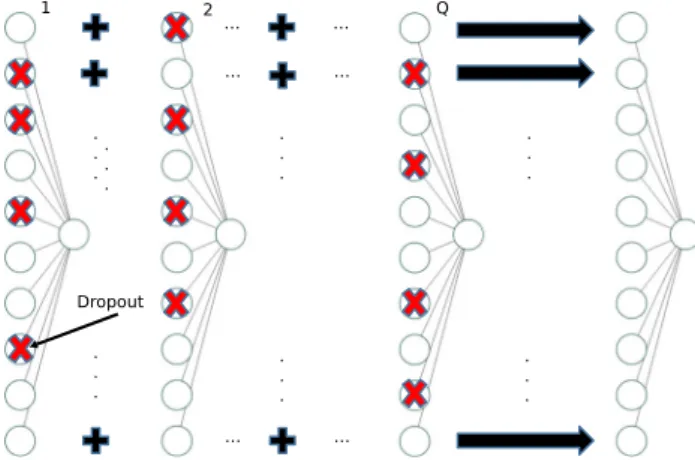
literature, the paper presents a procedure that limits the computational cost of the training phase on these devices. The proposed approach determines the eventual linear predictor for a network withNhidden neurons by merging an ensemble of Q linear predictors; each element of the ensemble is a network holding N~\N neurons. Figure1 outlines the underlying architecture. The contribution of each neuron (i.e., its weight) in the eventual network results from the summation of the non-dropped corre-sponding weights in each sub-network.
As compared with the methods cited above
[23, 25, 27, 51], this schema exhibits a hybrid ensem-ble/dropout training procedure, which best exploits the regularization properties of the dropout process, while limiting the computational cost of the training process.
The empirical validation on a set of eight well-known benchmarks and three real-world datasets recently used to test IoT algorithms confirmed that the proposed method could yield a satisfactory trade-off between generalization performances and hardware requirements for training. To prove the effectiveness of the electronic design, the train-ing algorithm was implemented on a pair of low-power, resource-constrained devices, namely the Broadcom BCM2837B0 Quad–core Cortex-A53, and an Allwinner H3, Quad–core Cortex-A7.
1.1 Contribution
The major contributions of the approach described in this paper can be summarized as follows:
• A novel training algorithm for RBN classifiers, featur-ing a low-cost optimization procedure that yet preserves the generalization ability of the eventual predictors. • A design strategy to support the training of RBNs in
embedded devices.
• For a given training set and a specified network size, an analytical formulation of the cost function yields a
preliminary assessment of the required number of operations when implemented in commercial devices. • The demonstration of the method effectiveness in two
main stream devices for IoT applications and 11 real-world benchmarks.
The paper is organized as follows: Sect.2reviews both the ELM model and the dropout regularization scheme. Sec-tion 3 illustrates the novel training strategy, also in com-parison with related works. Sections4and5 report on the experimental results, whereas some concluding remarks are made in Sect.6.
2 Background
2.1 Extreme learning machine
The ELM model features a vast, long-standing literature within the existing RBN approaches. Let X be the input domain (typically, X 2RD, D2Nþ), while T ¼ fðx;yÞi;x2 X;y2 f1;1g;i¼1;. . .;Zg denotes a
labeled training set drawn i.i.d. from a fixed, unknown distribution,P.
The parameters of the hidden layer ðbj2RD;bj2
RÞ;j¼1;. . .;Nare random; hence, the layer implements a fixed mapping of the input space,X, into RN. The ELM
training process optimizes the output weights x2RN by
solving a regularized least square (RLS) problem in the remapped space [17]. Let H denote the activation of the hidden layer as aZN matrix, wherehij¼hjðxi;bj;bjÞis
the activation of thejth neuron for theith input sample and Z is the number of samples in the training set. Then, the associate learning problem can be expressed as
min
x fkyHxk
2
þkkxk2g ð1Þ
WhenZN, one has:
x¼HTðkIþHHTÞ1y ð2Þ Conversely, whenZ[N, one has:
x¼ ðkIþHTHÞ1HTy ð3Þ In the following, it will be assumedZ[Nwithout loss of generality. The eventual classifier can be written as
y¼sign X N j¼1 xjhjðxi;bj;bjÞ ! : ð4Þ
2.2 Dropout regularization
The dropout technique was first introduced in [43] to tackle the overfitting problem, which affects the training of fully connected networks when adopting iterative algorithms.
For a single-layer, fully connected network trained with a gradient descend algorithm, the quantity Ht will denote the activation of the hidden layer at thetth iteration of the training process. The dropout procedure ignores a subset of neurons at each training iteration that subset varies from one iteration to another. A vectorm2 f0;1gNof Bernoulli random variables keeps track of such mechanism: at each iteration, the variable mj {j = 1,...,N} takes on the values
f1;0gwith probabilitiesp, 1p, respectively. At iteration t, the vector mt is drawn at random, and it multiplies
ele-ment-wise the columns of matrix Ht. Thus, the
contribu-tions of all neurons whose multipliers inmtare zero nullify for that iteration.
A major advantage of dropout is that the resulting net-work actually represents the (sparse) average of an ensemble of smaller networks; this notably simplifies the overfitting problem. Moreover, the dynamic exclusion mechanism makes it less likely that an input sample strictly corresponds to one specific neuron of the network. As a consequence, the solution of the optimization problem gets more robust even when a specific neuron is removed.
2.3 Dropout extreme learning machine
Iosifidis et al. [21] recently applied the concept of dropout regularization to extreme learning machines and proposed an augmented loss function to set the learning process:
L ¼1 2trðx TS xÞ þc 2kyHxk 2 þ k 2NT XNT t¼1 kHt^xk2 ð5Þ
The first term in the expression (5) aims to regularize the output weights x and takes into account the geometrical information of the input space through the use of matrixS; this term is not related to the dropout mechanism. The conventional mean square error characterizes the second term. The third term takes into account the NT
sub-net-works; it includes the matrix H^ ¼HH0, where H0 is
obtained from matrixHby setting a set of rows to 0 and is expected to introduce benefits of dropout mechanisms into the eventual classifier. The weighting hyper-parameters c and k balance the contributions of the corresponding terms.
The minimum of (5) is written as
x¼ HTHþk cR1þ 1 cS 1 HTy ð6Þ where
R1¼ 1 NT XNT t¼1 ^ HTtH^t ð7Þ
The summation becomes an expectation when NT! 1;
hence, one has
R1¼ ðHTHÞ P ð8Þ
whereP¼ ½ðpTpÞ 1T1I þ ½ð1TpÞ I; herepis a row
vector with the dropout probability of each neuron,1 is a row vector whose elements are all equal to 1, anddenotes the element-wise product.
The formulation (5) leads to a closed-form solution:
x¼ ½HTH 1T1þk cP þ1 cS 1 HTy ð9Þ
It is worth noting that—in terms of asymptotic computa-tional complexity—this solution exhibits the same com-plexity of the expression (3). Section 3.2 analyzes the associate computational costs in detail.
3 Constrained ensemble-based training
procedure
3.1 Dropout and local ensemble for efficient
training
The first step of the training procedure complies with the basic ELM model: a set ofNneurons remaps the training set,T, into a spaceH2RZN. The quantitiesZandNset the size of the matrixH.
The constrained ensemble-based approach now applies a sub-sampling of the matrixH. At each stepq of the sub-sampling process, a subset of rowsZ~and columns N~are drawn at random and considered to evaluate the cost function. The idea of using a subset of N~ neurons intro-duces the dropout mechanism. This leads to a reformulated training problem: min ~ xq ky~qHq~ x~qk2þkkx~qk2 n o ; q¼1;. . .;Q: ð10Þ The reduced vector of target classes, y~q, is obtained by removing fromythe target values associated with the rows that have been disregarded inH. Reducing the size of the input set clearly speeds up training. In addition, by sub-sampling the training set one limits the correlation among predictors, thus enhancing the generalization performance of the overall ensemble.
To clarify the advantages of the sub-sampling process, one might rewrite the optimization problem (10) in terms of the full matrix:
min x0 q y0qH0qx0q 2 þkkx0qk2 ; q¼1;. . .;Q: ð11Þ In the matrices H0 q2R ZN and y0 q2R Z, the elements
corresponding to the rows/columns disregarded in the qth sub-sampling iteration (10) nullify. Thus, the training process (11), characterized by explicit sparseness, involves a matrixH0
q with sizeZN. By contrast, the formulation
(10) just requires to trainQpredictors, each associated with one of Q sub-problems. To obtain the solutionx0
q of the
complete problem (11), one augments each vector x~q by
introducing null elements in correspondence of those neurons that had been disregarded in the sub-sampling step.
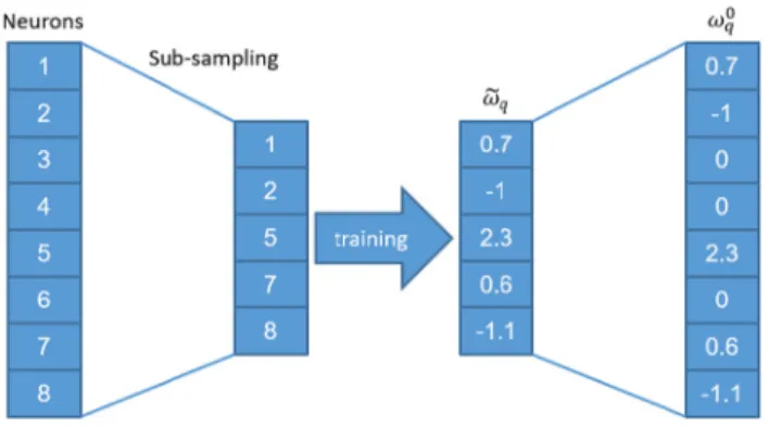
Figure2illustrates the computation ofx0
qfromxq, in a
demo network with N¼8 neurons. In the example, the sub-sampling procedure shrinks the number of neurons to
~
N¼5, and the training algorithm works out the predicted values x~q for the 5 neurons. The overall predictor x0q is
then worked out by padding the solution with zeros in correspondence of the indices that have been excluded by the sampling process.
The eventual predictor for the explicit space H is obtained by summing up theQlinear predictorsx0
q: fðxÞ ¼hðxÞx¼X N n¼1 hnðxÞ XQ q¼1 x0n;q wherehðxÞ ¼ fh1ðx;b1;b1Þ;. . .;hNðx;bN;bNÞg ð12Þ
The overall vector x is assembled at the end of the
training process; hence, the computational cost of the network training during the inference phase remains unaffected, as compared with the basic ELM model.
Although the eventual predictor might appear similar to a local ensemble, as in dropout regularization [43], the proposed solution exhibits a few computational advan-tages. First, the Qsub-networks all share the same input space; as a result, the Q matrices H~q can all be derived
from H, which is only computed once. This reduces the
Fig. 2 Example showing the sub sampling mechanism and the conversion fromx~q
load that would be required by the explicit mapping ofH~q
in each predictor. In addition, the overall prediction results from the activation of one network rather than by adding the predictions of all sub-networks. As a consequence, the eventual prediction inherently embeds a weighting mech-anism that characterizes refined ensemble strategies.
Algorithm 1 outlines the overall training procedure.
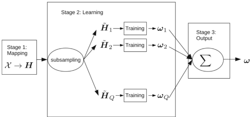
Figure3illustrates Algorithm 1 in a graphic form. The three boxes in the graph correspond to the three steps of the algorithm. After remapping the training data (Mappingbox in the figure), the matrixHis sub-sampledQtimes and the Q optimization problems are solved independently (Learning box). The schema highlights the parallel
computations of the simpler Q problems, which can therefore be supported by resource-constrained devices by means of multiprocessing. The final step (Output box) merges the individual linear separators to work out the overall predictorx.
3.2 Analysis of computational cost
Several issues hinder the training of a SLFNN on resource-constrained devices. The expression (3) sets the computa-tional cost for both the standardL2 regularized ELM and the proposed approach. Nonetheless, solving (9) involves
Fig. 3 Flow graph of Algorithm 1
Algorithm 1Drop out ensemble based learning algorithm
Input
• a labeled training setT ={(x, y)i;i= 1, ..., Z}
• number of neuronsN
• number of iterationQ
• number on neurons subset ˜N
• number on training sample subset ˜Z
0.Initialize
initialize a pool ofNrandom neurons
1.Mapping
remap all the patternsx∈ T by using the random neurons
h(x) ={h1(x,β1, b1), ..., hN(x,βN, bN)} 2.Learning
forq=1; q=<Q; q++do
extract random sample ˜H∈H, ˜y∈y
train a linear predictor: ˜ωq= (λI+ ˜HTH˜)−1H˜Ty˜
compute equivalent solutionω0q
end for
3.Outputcompute linear predictor in the space
ω∗= Q q
ω0 q
an additional computational overhead; at the same time, memory occupation and latency bring about the major constraints and are affected by multiple factors.
3.2.1 Input data remapping
The first step in RBN training is the remapping of the input data, which can be formalized as
H¼signðXtrainbþrepmatðb;½Z;1ÞÞ ð13Þ
whereb2RZNandb2RN1are the network parameters, and the repmat operator just appends the bias value,b, to each training datum. The number of multiplications and additions scales as OðZNDÞ. When adopting linear approximations [30], the computation of NN nonlinear terms requires a minimum of 2NN additional oper-ations. The number of operations increases if one involves more accurate approximations.
3.2.2 Optimization
Then, one tackles the actual optimization problem in the remapped space. Two main sub-steps determine the asso-ciate computational time: the matrix multiplication HTH
and the solution of the associate system of linear equations. Different strategies can apply depending on the hardware resources available: for example, the matrix multiplication can be carried out in parallel.
In the ideal case of unbounded computational resources, the matrix multiplication can complete in two clock cycles: first, a set ofZparallel HW units carry out individual inner products (to compute each element of the result); then, the resulting individual terms feed an adder circuit having Z inputs. By using N2 of such product/adder blocks and
assuming that each multiplication/addition completes in 1 clock cycle, the overall process completes in 2 clock cycles. Such an unrealistic solution just sets an upper bound to timing performance. Conversely, in an opposite, worst-case HW configuration including one floating point unit, the best known computational bound is OðN2:37286Þ [24] for a pair of square matrices. Again, such a setup seems unrealistic because the largest term in the compu-tational cost scales asaN2:37286, wherea[ [N2:37286 for
reasonable values of N. As a consequence, the method proposed in [24] becomes convenient only when the matrices are asymptotically large. The literature offers several practical approaches, based on the number of computational units, memory structures, and memory size. Conventional solutions rely on the Strassen matrix multi-plication algorithm, which scales as OðN2:807Þ [16]. A
speedup is obtained, for square input matrices, when the matrix size is larger than 100; that algorithm also scales
efficiently for the rectangular matrices,H, that characterize the training process.
The solution of a linear equation system is less prone to a parallel approach. Existing algorithms scale as the third power of the number of variables (i.e., the number of neurons N). The literature shows that Singular Value Decomposition (SVD) [17] yields satisfactory numerical solutions, whose computational cost can be roughly approximated by 12N3[13]. The linear equation system in Eq. (3) just involves a matrixðHTHþkIÞthat is Hermitian and reasonably well conditioned. This allows to adopt Cholesky decomposition as a reference model in terms of memory and computational cost. This procedure scales as N3=3 and proves more efficient than the conventional LU
factorization 2N3=3. A forward and backward substitutions are eventually required to complete the procedure, intro-ducing 2N2 additional operations.
3.2.3 Model selection
The model selection strategy heavily affects the overall cost of the training process. A naive approach to model selection would require to iterate a number of training procedures, each characterized by as many settings of the hyper-parameters.
When considering k, the pair of matrix multiplications
HTH and HTy in the expression (3) need not be
recom-puted for different values of k. Likewise, by using SVD one need not work out again the matricesU,S,V, since the summation with the diagonal matrix kI only affects the elements of S[13]. SVD efficiently supports spectral reg-ularization techniques [12], as well. On the other hand, the Cholesky algorithm requires to carry out the complete procedure for each setting ofk.
The number of trials required to set the number of neurons,N, is critical to determine the computational cost. The eventual procedure benefits from the properties of matrix multiplications, which allow one to avoid the re-computation of the whole matrix HTH as part of the learning process [13].
In typical on-board IoT applications, the number of neurons and the size of the training set are not asymptoti-cally large due to memory constraints. As a result, the overall approximation of the cost function needs to be fine grained. In the case of L2-regularized ELMs, the expres-sion (14) gives an adequate approximation of the number of floating point operations required for training:
OL2ðN;ZÞ ¼OðHTHÞ þOðHTyÞ þkðOðHTHþkIÞ þOðlinsolveðHTHþkI;HTyÞÞ þOðHvalxÞÞ ¼N2ZþNZþk NþaNnþcþZvalN ð14Þ where linsolve operator embeds the solution of the linear equation system that is identified by (aNnþc) and k is
the number of different settings for the hyper-parameterk. For each value of k, the predictor is computed over the validation set, marked with the subscript ‘‘val’’ in (14). The proposed equation considers all the matrix–matrix and matrix–vector operations involved in the solution of the learning problem (1). One might argue that (14) does not take into account the model selection for the parameterN; this seems a reasonable assumption when addressing resource-constrained devices, where N is limited due to hardware constraints.
The computation of (9) also requires to work out matricesPandS. Moreover, the model selection procedure optimizes three hyper parameters: k; c and p. As a con-sequence, the expression (14) actually sets a lower bound to the computational complexity of both (9) and (6). 3.2.4 Overall computational cost
In the novel training procedure proposed in this paper, the mapping phase matches the basic model. Instead, the augmented cost function (11) involves the second phase of the training process after remapping. Thus, the overall computational cost of the approach proposed in this paper can be written as
Odrop¼QðOL2ðN~;Z~ÞÞ: ð15Þ
where N~ and Z~are the size of the sub-sampled sets of neurons and training data, respectively.
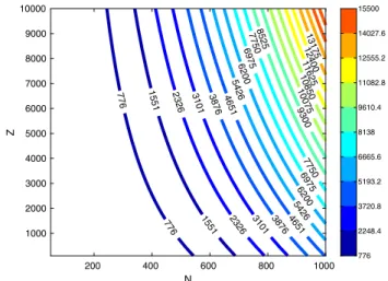
The expression (15) shows that the proposed approach is most effective when Q is small. The term Q affects the overall cost almost linearly, whereas the impact of quan-titiesZ~\Z andN~\Nis quadratic and cubic, respectively. In this regard, Fig. 4 shows the behavior of the cost function (14) for different values of the parametersZ and N. The graph confirms that the computational cost rapidly decreases asZandNdecrease.
Interestingly, the eventual speedup of the training phase presented in [51] becomes marginal as compared with that obtained by the approach proposed in this paper. Further-more, the forward phase of the predictors presented in [51] requires time-consuming operations such as sorting. As a result, the predictor [51] proves more computationally demanding than traditional SLFNNs.
3.3 Comparison with related works
Ensemble approaches combined with RBNs [23, 25, 27] usually aim to enhance generalization performance disre-garding the associate computational cost. State-of-the-art works do not set constraints on the number of neurons of the overall ensemble. As a consequence, both memory occupation and latency of the inference phase increase. The solution proposed here, instead, aims to balance general-ization performances and computational cost: it sets the size of the hidden layer,N, a priori, based on the available memory. Then, individual learners all sample the random neurons from the same pool. Finally, learners merge into a single network, i.e., the eventual classifier, having size N. As a consequence, the inference phase has the same computational cost of standard feed-forward networks with Nneurons.
The proposed approach outperforms state-of-the-art dropout-based methods in terms of computational cost. In [51], an additional fuzzy logic affected the computational complexity of the training phase. Furthermore, the forward phase of the predictors required complex operations such as sorting; hence, the classifier proved less efficient than traditional SLFNNs.
In [21], the authors introduced a novel regularization term, and the cost function still involved the solution of a linear equation system. This operation roughly scales as N3. Conversely, in the proposed approach the training
procedure involves a subset of Qproblems that scales as ~
N3. The results presented in Sect.4 will confirm that sat-isfying results can be achieved with QN~3\\N3. In
addition, Algorithm 1 highlights a crucial difference with respect to the approach presented in [21], where the authors
776 776 1551 1551 2326 2326 3101 3101 387 6 38 76 4651 4651 5426 5426 6200 6200 6975 6975 7750 7750 8525 9 300 10075 10 850 116 2 5 12400 13175 200 400 600 800 1000 N 1000 2000 3000 4000 5000 6000 7000 8000 9000 10000 Z 776 2248.4 3720.8 5193.2 6665.6 8138 9610.4 11082.8 12555.2 14027.6 15500
Fig. 4 Value of functionOL2for different combinations of parameter ZandN, withc¼13. The numerical values are normalized using the
values of the smallest considered network
focused on the minimization of (5) and forced the solution
x to be valid for any sub-network (obtained by dropout procedure) and the original complete network. By contrast, the procedure proposed in this work obtains the solution by combining a set of independent learners. Using a subset of training data, one might affect the regularization properties of the dropout method. At the same time, theQ -indepen-dent learners are expected to be orthogonal to a certain extent. This in turn should increase the generalization ability of the eventual ensemble and limit the risk of overfitting accordingly [33].
When considering electronic implementations, the method proposed in this paper addresses the efficient deployment on inexpensive devices. The related design approaches typically aimed efficient digital implementa-tions of RBNs in configurable architectures. A very large-scale integration (VLSI) architecture was the main target in [3, 6]; the approach presented in [32] envisioned analog implementations and combined a tri-state activation func-tion with an offline pruning procedure to limit the predictor complexity. The models proposed in [9, 10, 37, 50] tar-geted FPGA implementations of the learning phase, either online or in batch mode. Conversely, Decherchi et al. [7] and Ragusa et al. [35] proposed a minimal implementation of the forward phase of RBNs, while [32,49] introduced an effective scheme to reduce the memory requirements of the eventual predictors.
4 Generalization performances
To evaluate the generalization effectiveness of the pro-posed method, an experimental setup simulated a real use-case, in particular the size of the mapping layer was bounded by hardware constraints. Table 1 gives the main features of the 11 involved benchmarks, which were arranged in two sets: standard benchmarks and IoT benchmarks.
The proposed approach was compared with a pair of computational demanding solutions, namely an ELM with L2 regularization [18] and a dropout ELM [21]. Those algorithms represented the most interesting solutions in terms of trade-off between computational cost, general-ization performance, and impact of the hyper parameters.
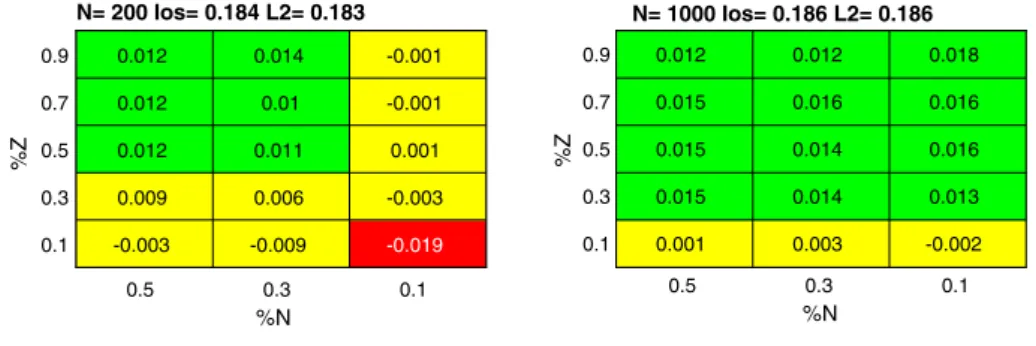
In the following, the presentation of the experimental results will always adopts a common format: for each experiment, a pair of sub-figures (a) and (b) will give the results obtained for different settings of the size,N, of the hidden layer. In all tables, rows will correspond to the size of the training sub-setZ~, whereas columns will refer toN~. The table rows/columns will give the settings with respect to the reference values, Z and N, respectively. Therefore, the topmost row will mark a predictor trained with Z~¼ 0:9Z and the leftmost column will indicateN~¼0:5N. The title of each table will give the percentage classification error, expressed in the range [0, 1] scored by both the dropout regularized solution (Ios) [21] and the L2
regu-larized network (L2), all holding N neurons. Table cells will give the discrepancy between the test error (averaged over 100 iterations) scored by the proposed method and the error attained by Ios regularized method:
Ti;j¼
1 100
X100 n¼1
ðIosnProposalnði;jÞÞ ¼IosProposal
ð16Þ whereTi;j is the table element, Ios is the test error of the
baseline [21] method using the nth random extraction of the hidden layer, and Proposalnði;jÞis the test error scored by the proposed method using the settingi,jand the pool of neurons belonging to thenth random hidden layer.
Positive values will be characterized by a green cell background and will indicate that the hardware-friendly dropout strategy scored better results. The cells having a red background, instead, will mark those tests in which the proposed method did not outperform conventional ELMs. Yellow background cells will denote those settings in which the discrepancy between the comparisons was marginal (less than 1%).
The statistical significance of the results was measured considering the weak law of large numbers. All measures marked in green and red were statistically significant because jTi;jj[j2rIosj þ j2rProposalj, where rIos and
rProposal are the standard deviations of Ios and Proposal,
respectively.
Each experiment involved: two settings of the hidden layer size N¼ f200, 1000g, 13 values of the hyper-pa-rameter k¼10i;i¼ f6;5;. . .;6g, 3 values of the
parameterN~¼ f0:5;0:3;0:1gN, and 5 values for parameter ~
Z ¼ f0:9;0:7;0:5; 0:3;0:1gZ. The datasets were always Table 1 Dataset characteristics
Dataset Z D QSAR 1052 41 Pima 768 8 CreditCard 29,965 24 Ozone 1847 73 Ionosphere 350 34 HTRU 17,898 9 Blood 533 5 Australian 690 39 MNIST 1000 81 Ds2os 357,952 11 Fog 121,603 10
drawn by using a balanced configuration, in which the number of patterns was normalized to the least numerous class. Generalization performances were measured by using standard hold-out procedure. The training set was extracted by using 70% of the training data, whereas the validation and test set included 20%and 10%of the data, respectively. The parameter k was set accordingly to the best result scored on the validation set. Generalization performances are reported after measurements on test data, i.e., data that had never been used during either training or model selection. The following subsections illustrate the outcomes of the experiments for standard machine learning benchmarks and on IoT specific benchmarks.
Setting the iteration parameterQ= 10 limited the size of the experimental section. Indeed, that setting corresponded to the smallest value that proved sufficient in all the benchmarks to obtain stable results. This choice did not affect the validity of the results obtained on the test sets. As a matter of fact, the implementation analysis always con-sidered a worst-case scenario because, in most cases, the smallest value of Q that reached good performances was smaller than 10.
The reported results aim to confirm that the proposed algorithm could yield satisfactory accuracy values (as compared with the reference approaches) but at a smaller computational cost of the training process.
4.1 Standard machine learning benchmarks
The first set of experiments included 8 popular benchmarks for machine learning, all drawn from the UCI repository [8], mostly to allow fair comparisons with existing approaches.
The results on the QSAR dataset (Fig.5) scored a lim-ited gap (less than 3%) in performance between the pro-posed approach and the two baseline comparisons. Remarkably, the hardware-friendly dropout strategy proved equivalent or even more effective in terms of generalization performances.
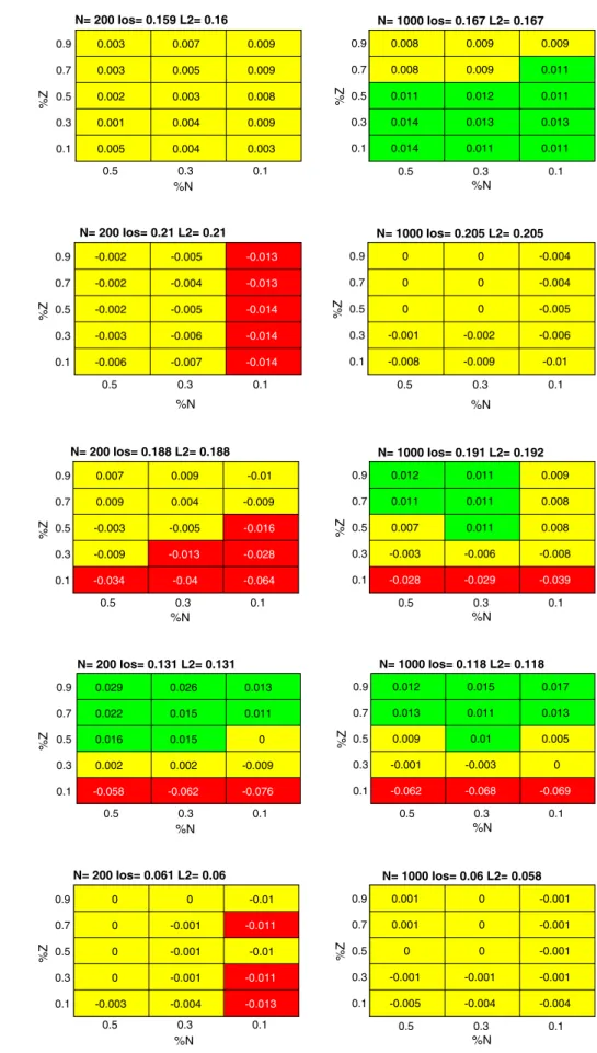
The data presented in Fig.6 refer to the Pima-Indians dataset. The results were similar to those shown in Fig.5 and confirmed that the proposed dropout scheme could
limit overfitting significantly in the presence of small sub-networks. Remarkably, this configuration was most con-venient in terms of hardware requirements.
Figure 7 gives the results obtained on the ‘‘Default of credit card clients’’ dataset. Although the proposed strategy seemed to yield lower performances, the gap always kept quite small; it was smaller than 0:1%in six cases and lower than 1% in the majority of the others. The minor degra-dation in performances was largely compensated by the hardware effectiveness of the supporting architecture.
The results on the Ozone dataset (Fig.8) highlight the crucial trade-off between the performances of the base classifiers (i.e., the sub-networks trained independently) and those of the overall eventual predictor. Small sub-networks trained on small data chunks usually obtained unsatisfactory results (up to 6%of error increment). Con-versely, when the sizes of the sub-networks and of the data chunks increased, the performances of the eventual clas-sifiers got comparable or even better with the baseline solutions, with gaps smaller than 1%.
The tests on the Ionosphere dataset (Fig.9) exhibited a similar trend forZ~. Such a behavior was due to the fact that this benchmark held a limited number of samples; con-versely, when %Z exceeded 30%, the proposed approach proved more convenient.
The differences between the comparisons were almost negligible in all the configurations for the HTRU dataset (Fig. 10). The gap was negligible also in profitable hard-ware configurations, i.e., when bothZ~andN~took on small values.
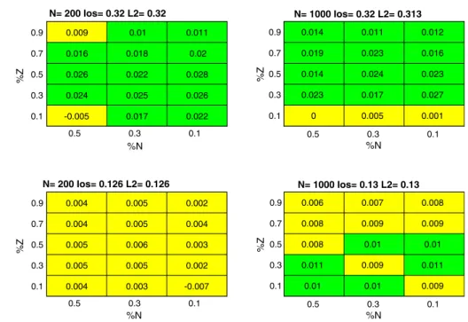
When tested on the Blood dataset (Fig.11), the present approach proved to be the best solution in almost all con-figurations. Finally, the results on Australian Credit Card dataset (Fig.12) confirmed that the proposed solution could attain performances that always closely approximated those achieved by the baseline algorithms.
4.2 Internet of Things benchmarks
These benchmarks belonged to a corpus of recent machine learning papers for IoT, and covered a wide spectrum of
0.5 0.3 0.1 0.9 0.7 0.5 0.3 0.1 %Z N= 200 Ios= 0.184 L2= 0.183 0.012 0.012 0.012 0.009 -0.003 0.014 0.01 0.011 0.006 -0.009 -0.001 -0.001 0.001 -0.003 -0.019 0.5 0.3 0.1 %N %N 0.9 0.7 0.5 0.3 0.1 %Z N= 1000 Ios= 0.186 L2= 0.186 0.012 0.015 0.015 0.015 0.001 0.012 0.016 0.014 0.014 0.003 0.018 0.016 0.016 0.013 -0.002 Fig. 5 QSAR biodegradation
0.5 0.3 0.1 %N 0.9 0.7 0.5 0.3 0.1 %Z N= 200 Ios= 0.159 L2= 0.16 0.003 0.003 0.002 0.001 0.005 0.007 0.005 0.003 0.004 0.004 0.009 0.009 0.008 0.009 0.003 0.5 0.3 0.1 %N 0.9 0.7 0.5 0.3 0.1 %Z N= 1000 Ios= 0.167 L2= 0.167 0.008 0.008 0.011 0.014 0.014 0.009 0.009 0.012 0.013 0.011 0.009 0.011 0.011 0.013 0.011 Fig. 6 Pima-Indians Diabetes
dataset 0.5 0.3 0.1 %N 0.9 0.7 0.5 0.3 0.1 %Z N= 200 Ios= 0.21 L2= 0.21 -0.002 -0.002 -0.002 -0.003 -0.006 -0.005 -0.004 -0.005 -0.006 -0.007 -0.013 -0.013 -0.014 -0.014 -0.014 0.5 0.3 0.1 %N 0.9 0.7 0.5 0.3 0.1 %Z N= 1000 Ios= 0.205 L2= 0.205 0 0 0 -0.001 -0.008 0 0 0 -0.002 -0.009 -0.004 -0.004 -0.005 -0.006 -0.01 Fig. 7 Default of credit card
clients dataset 0.5 0.3 0.1 %N 0.9 0.7 0.5 0.3 0.1 %Z N= 200 Ios= 0.188 L2= 0.188 0.007 0.009 -0.003 -0.009 0.009 0.004 -0.005 -0.01 -0.009 -0.034 -0.013 -0.04 -0.016 -0.028 -0.064 0.5 0.3 0.1 %N 0.9 0.7 0.5 0.3 0.1 %Z N= 1000 Ios= 0.191 L2= 0.192 0.012 0.011 0.007 -0.003 0.011 0.011 0.011 -0.006 0.009 0.008 0.008 -0.008 -0.028 -0.029 -0.039
Fig. 8 Ozone dataset
0.5 0.3 0.1 %N 0.9 0.7 0.5 0.3 0.1 %Z N= 200 Ios= 0.131 L2= 0.131 0.029 0.022 0.016 0.002 0.026 0.015 0.015 0.002 0.013 0.011 0 -0.009 -0.058 -0.062 -0.076 0.5 0.3 0.1 %N 0.9 0.7 0.5 0.3 0.1 %Z N= 1000 Ios= 0.118 L2= 0.118 0.012 0.013 0.009 -0.001 0.015 0.011 0.01 -0.003 0.017 0.013 0.005 0 -0.062 -0.068 -0.069
Fig. 9 Ionosphere dataset
0.5 0.3 0.1 %N 0.9 0.7 0.5 0.3 0.1 %Z N= 200 Ios= 0.061 L2= 0.06 0 0 0 0 -0.003 0 -0.001 -0.001 -0.001 -0.004 -0.01 -0.01 -0.011 -0.011 -0.013 0.5 0.3 0.1 %N 0.9 0.7 0.5 0.3 0.1 %Z N= 1000 Ios= 0.06 L2= 0.058 0.001 0.001 0 -0.001 -0.005 0 0 0 -0.001 -0.004 -0.001 -0.001 -0.001 -0.001 -0.004 Fig. 10 HTRU dataset
configurations, ranging from small size to medium-/high-size problems.
The MNIST dataset addressed the recognition of hand-written digits; as in previous works [7], the research pre-sented here used a reduced version of that dataset, including 1000 patterns represented by 99 grey-scale images. The bi-class classification problem involved the (most difficult) discrimination task between digits ‘‘3’’ and ‘‘8.’’ A similar setup was recently adopted in [48], pre-senting an IoT learning algorithm for visual patterns.
Distributed smart space orchestration system (Ds2os) was the second IoT-related benchmark and included a collection of traces captured in a networking domain for IoT.1 The data had been collected from the application layer; hence, they differed significantly from the conven-tional feature-based patterns used by network-traffic clas-sifiers. The main dataset included various sources, such as light controllers, thermometers, person detection sensors, washing machines, batteries, thermostats, smart doors, and smart phones. In compliance with the comparative approach proposed in [15], the binary problem set in this paper discriminated normal activity vs anomalies.
The freezing of gait (Fog) dataset [2] held the annotated readings of 3 acceleration sensors (positioned at the hips and legs) of patients affected by the Parkinson disease, who could experience freezing of gait during walking tests.
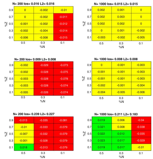
The results for the IoT benchmarks are reported in Figs.13,14and15. For the MNIST database, experimental outcomes in Fig. 13 confirmed the method effectiveness. The baseline comparisons only performed better in the case
%N¼0:1, whereas in most cases, the differences in per-formances never exceeded 1%. On the other hand, the dropout strategy for IoT devices featured a considerable speedup of the learning procedure.
The results in Fig.14for the Ds2os benchmark highlight the role of the pool size,N. In the configurations involving N¼200 with small values of N~, the proposed hardware-friendly method exhibited a non-negligible loss in term of accuracy. This drawback almost vanished in configurations withN¼1000, as the loss in accuracy always kept smaller than 1%, with the already remarked advantage of a smaller computational cost.
The results for the Fog dataset (as per Fig.15) showed a similar trend. The loss in accuracy proved significant when N¼200 and N~\0:5N. In practical scenarios, however, involving networks with a consistent set of neurons, the accuracy values matched those attained by standard approaches. From this viewpoint, the two basic procedures L2and Ios scored an improvement in accuracy of about 4%
when the pool size increased from 200 to 1000. In the latter setup (N¼1000), the proposed approach outperformed the reference comparisons.
4.3 A summary of generalization results
Overall, generalization performances proved comparable with the results reported in the literature, although a direct, thorough comparison could not always be accomplished due to differences in the experimental setups.
The outcomes of the experimental session can be sum-marized as follows: 0.5 0.3 0.1 %N 0.9 0.7 0.5 0.3 0.1 %Z N= 200 Ios= 0.32 L2= 0.32 0.009 0.016 0.026 0.024 -0.005 0.01 0.018 0.022 0.025 0.017 0.011 0.02 0.028 0.026 0.022 0.5 0.3 0.1 %N 0.9 0.7 0.5 0.3 0.1 %Z N= 1000 Ios= 0.32 L2= 0.313 0.014 0.019 0.014 0.023 0 0.011 0.023 0.024 0.017 0.005 0.012 0.016 0.023 0.027 0.001 Fig. 11 Blood dataset
0.5 0.3 0.1 %N 0.9 0.7 0.5 0.3 0.1 %Z N= 200 Ios= 0.126 L2= 0.126 0.004 0.004 0.005 0.005 0.004 0.005 0.005 0.006 0.005 0.003 0.002 0.004 0.003 0.002 -0.007 0.5 0.3 0.1 %N 0.9 0.7 0.5 0.3 0.1 %Z N= 1000 Ios= 0.13 L2= 0.13 0.006 0.008 0.008 0.011 0.01 0.007 0.009 0.01 0.009 0.01 0.008 0.009 0.01 0.011 0.009 Fig. 12 Australian Credit Card
dataset
• In the experiments involving the standard benchmarks, the proposed approach attained generalization perfor-mances comparable with those scored by the baseline algorithms, (i.e., L2-regularized and dropout ELMs); the latter comparisons, however, proved much less efficient in terms of computational complexity. • The experiments involving IoT benchmarks confirmed
that trend, with the only exception of the Distributed smart space orchestrian system dataset. The gap between the configurations withN¼200 neurons and those holding N¼1000 neurons seems to suggest that this issue might be solved by using a larger hidden layer.
5 Implementation analysis
The implementations on embedded architectures involved a pair of popular, commercially available devices for IoT applications, that is, the Broadcom BCM2837B0 Quad-Core Cortex-A53 (characterized by 1.4 GHz clock
frequency, 32 kB L1 e 512 kB L2), and an Allwinner H3, Quad-Core Cortex-A7 (clock up to 1.2 GHz, equipped with 1 GB and 512 MB of RAM). These devices were selected because they supported well-known IoT devices, namely the Raspberry Pi 3b?and the NanoPi NEO AIR-Friendly ARM.
The experimental setup took into account the impact of the quantities Z~ and N~ on the latency of the proposed method in IoT applications. The campaign simulated the training process by using a toy procedure, and input data were generated at random. The tests considered a pair of settings of the training set size: Z¼ f500;2000g and two configurations of the hidden layer: N¼ f200;1000g. Generalization performances were not an issue here because the proposed devices adopted the floating point representation and the focus was on computational effi-ciency. The algorithms were all implemented in Python by using the Numpy library.
In the following, all the results will be arranged according to the size of the input layer. Each figure will include a pair of graphs, one for each setting of the train-ing-set size, Z. The x-axis will group the results based on
0.5 0.3 0.1 %N 0.9 0.7 0.5 0.3 0.1 %Z N= 200 Ios= 0.016 L2= 0.016 0 0 -0.001 -0.002 -0.006 -0.002 -0.002 -0.002 -0.004 -0.008 -0.01 -0.011 -0.012 -0.014 -0.015 0.5 0.3 0.1 %N 0.9 0.7 0.5 0.3 0.1 %Z N= 1000 Ios= 0.015 L2= 0.015 0.002 0.002 0.002 0 -0.003 0.001 0.003 0.002 0.001 -0.002 0 0 0 -0.002 -0.005 Fig. 13 MNIST dataset
0.5 0.3 0.1 %N 0.9 0.7 0.5 0.3 0.1 %Z N= 200 Ios= 0.009 L2= 0.008 -0.002 -0.002 -0.003 -0.003 -0.005 -0.029 -0.028 -0.028 -0.028 -0.026 -0.073 -0.075 -0.078 -0.074 -0.074 0.5 0.3 0.1 %N 0.9 0.7 0.5 0.3 0.1 %Z N= 1000 Ios= 0.008 L2= 0.008 0 -0.001 -0.001 -0.002 -0.004 -0.001 -0.001 -0.001 -0.001 -0.005 -0.003 -0.003 -0.003 -0.004 -0.006 Fig. 14 Distributed smart space
orchestration system dataset
0.5 0.3 0.1 %N 0.9 0.7 0.5 0.3 0.1 %Z N= 200 Ios= 0.239 L2= 0.227 -0.01 -0.007 -0.001 0.018 -0.013 -0.035 -0.033 -0.032 -0.028 -0.013 -0.081 -0.079 -0.079 -0.079 -0.079 0.5 0.3 0.1 %N 0.9 0.7 0.5 0.3 0.1 %Z N= 1000 Ios= 0.211 L2= 0.183 0.019 0.021 0.022 0.023 0.019 0.006 0.008 0.012 0.017 0.017 -0.01 -0.04 -0.038 -0.035 -0.029 Fig. 15 Freezing of gait dataset
three settings of the hidden layer of the sub-networks: f0:5N;0:3N;0:1Ng. Each group involved five configura-tions of the parameterZ~. As a consequence, the left-most bar always will refer to the most demanding configuration, whereas the right-most bars will mark the most prof-itable settings. The y-axis will show the values of h¼Tproposal
TL2 , where Tproposal is the training time of the pro-posed approach andTL2 is the training time of a L2 basic
classifier. Thus, values ofh\1 andh[1 will indicate that the proposed solution proved faster or slower, respectively. The horizontal red line will mark the case whenh¼1. The L2 regularized network was adopted as a reference
com-parison because—according to the analytical analysis of the computational cost—it proved more efficient than the solution proposed in [21].
The first experiment involved the Quad-Core Cortex-A7 with 500 MB of RAM memory. The entire training process was supported by core 1; hence, no parallelism was exploited. This experimental setup simulated a heavily constrained scenario; the amount of resources involved was considerably smaller than those available on an average smartphone. Figure16gives the results for the configura-tion withN¼200. The proposed approach proved extre-mely convenient in term of latency. The cost always kept lower than 10% in all the configurations with N~¼0:1N. Interestingly, the advantage for the configuration with the highest computational load, N~¼0:5N and Z~¼0:9Z, approximated the best value 1. On the other hand, setting Q¼10 implied a worst-case analysis. Figure17considers the same hardware setup with a different size of the hidden layer, i.e., N¼1000. The experimental result showed a similar trend to the experiments reported previously.
The second set of implementation configurations involved the Quad-Core Cortex-A53 with 1 GB of RAM memory. As in previous tests, only one core of the Cortex-A53 was enabled. The major difference in this setup was the amount of memory (twice as much as compared with the Cortex A-7 tests).
Figures 18 and 19 present the related outcomes. The graphs show that the dropout-based strategy still attained remarkable speed-up values for configurations with N~¼ 0:1N and N~¼0:3N when Z ¼500. When Z¼2000, the speedup kept comparable with the performances scored in the presence of limited training sets (i.e., less than 1000). Simulations always addressed a worst-case analysis, in whichQ¼10.
The final experimental setup involved configurations that fully exploited the available hardware resources. The
proposed strategy relied on multi-threading; a thread was instantiated for each sub-network. Such an approach clearly implied a larger memory (RAM) consumption (Qtimes bigger), since the threads were expected to run in parallel. The number of available cores (4) set the corre-sponding best possible speedup value. For this reason, only the Quad-Core Cortex-A53 with 1 GB of RAM memory was used for these experiments.
Figures 20and21 report on the results of the tests for N¼200 andN¼1000, respectively. The reported results point out the advantages in latency featured by the pro-posed method in the configurations with 0.3N and 0.1N. The configuration 0.5N actually suffered from the limited available RAM; this prevented an efficient execu-tion of multiple tasks in parallel.
The outcomes of the experimental session about HW implementation can be summarized as follows:
• In the presence of tight memory constraints, the proposed solution scored remarkable speedup values in almost all configurations.
• When more relaxed memory constraints were allowed, as per Figs.18and19, the speed-up performances still proved significant when the networks sizes kept smaller than 0.3N. In the other cases, the values assumed by Qbrought about a significant impact.
• When applying multiprocessing, as per Figs.20and21, the implementations confirmed that the amount of shared memory influenced the speed-up performances. Finally, it is worth noting that the configurations (involving
~
NandZ~) that resulted most profitable in terms of hardware implementation also proved most effective in terms of generalization performances.
6 Conclusions
The paper proposed a novel training procedure for RBN in resources-constrained scenarios. The focus of the proposed method was the trade-off between generalization perfor-mances and the computational cost of the training phase. The major outcome of the described research consists in showing the feasibility and effectiveness of the proposed method to implement the learning phase on IoT devices. Extensive experiments have confirmed the satisfactory generalization performances of the proposed strategy. In particular, an extensive implementation analysis confirmed the feasibility of the proposed approach in low-power devices.
Z=500 0.5 0.3 0.1 %N 0 0.5 1 1.5 0.9Z 0.7Z 0.5Z 0.3Z 0.1Z thr Z=2000 0.5 0.3 0.1 %N 0 0.5 1 0.9Z0.7Z 0.5Z 0.3Z 0.1Z thr Fig. 16 Latency measured on
single core of Quad-Core Cortex-A7 with 500 MB of RAM memory withN¼200
Z=500 0.5 0.3 0.1 %N 0 0.5 1 0.9Z 0.7Z 0.5Z 0.3Z 0.1Z thr Z=2000 0.5 0.3 0.1 %N 0 0.5 1 0.9Z 0.7Z 0.5Z 0.3Z 0.1Z thr Fig. 17 Latency measured on
single core of Quad-Core Cortex-A7 with 500 MB of RAM memory withN¼1000
Z=500 0.5 0.3 0.1 %N 0 0.5 1 1.5 2 0.9Z 0.7Z 0.5Z 0.3Z 0.1Z thr Z=2000 0.5 0.3 0.1 %N 0 1 2 3 0.9Z 0.7Z 0.5Z 0.3Z 0.1Z thr Fig. 18 Latency measured on
single core of Quad Core Cortex-A53 with 1 GB of RAM memory withN¼200 Z=500 0.5 0.3 0.1 %N 0 0.5 1 1.5 0.9Z 0.7Z 0.5Z 0.3Z 0.1Z thr Z=2000 0.5 0.3 0.1 %N 0 0.5 1 1.5 2 0.9Z 0.7Z 0.5Z 0.3Z 0.1Z thr Fig. 19 Latency measured on
single core of Quad Core Cortex-A53 with 1 GB of RAM memory withN¼1000 Z=500 0.5 0.3 0.1 %N 0 0.5 1 1.5 2 0.9Z 0.7Z 0.5Z 0.3Z 0.1Z thr Z=2000 0.5 0.3 0.1 %N 0 0.5 1 1.5 2 0.9Z 0.7Z 0.5Z 0.3Z 0.1Z thr Fig. 20 Latency measured on
multi thread of Quad Core Cortex-A53 with 1 GB of RAM memory multi thread with N¼200
Funding Open access funding provided by Universita` degli Studi di Genova within the CRUI-CARE Agreement.
Compliance with ethical standards
Conflict of interest The authors declare that they have no conflict of interest.
Open Access This article is licensed under a Creative Commons Attribution 4.0 International License, which permits use, sharing, adaptation, distribution and reproduction in any medium or format, as long as you give appropriate credit to the original author(s) and the source, provide a link to the Creative Commons licence, and indicate if changes were made. The images or other third party material in this article are included in the article’s Creative Commons licence, unless indicated otherwise in a credit line to the material. If material is not included in the article’s Creative Commons licence and your intended use is not permitted by statutory regulation or exceeds the permitted use, you will need to obtain permission directly from the copyright holder. To view a copy of this licence, visithttp://creativecommons. org/licenses/by/4.0/.
References
1. Alaba PA, Popoola SI, Olatomiwa L, Akanle MB, Ohunakin OS, Adetiba E, Alex OD, Atayero AA, Daud WMAW (2019) Towards a more efficient and cost-sensitive extreme learning machine: a state-of-the-art review of recent trend. Neurocom-puting 350:70–90
2. Bachlin M, Plotnik M, Roggen D, Maidan I, Hausdorff JM, Giladi N, Troster G (2009) Wearable assistant for Parkinson’s disease patients with the freezing of gait symptom. IEEE Trans Inf Technol Biomed 14(2):436–446
3. Basu A, Shuo S, Zhou H, Lim MH, Huang GB (2013) Silicon spiking neurons for hardware implementation of extreme learning machines. Neurocomputing 102:125–134
4. Cao J, Lin Z, Huang GB (2012) Self-adaptive evolutionary extreme learning machine. Neural Process Lett 36(3):285–305 5. Chaturvedi I, Ragusa E, Gastaldo P, Zunino R, Cambria E (2018)
Bayesian network based extreme learning machine for subjec-tivity detection. J Frankl Inst 355(4):1780–1797
6. Chen Y, Yao E, Basu A (2015) A 128 channel 290 GMACs/W machine learning based co-processor for intention decoding in brain machine interfaces. In: 2015 IEEE International symposium on circuits and systems (ISCAS). IEEE, pp 3004–3007 7. Decherchi S, Gastaldo P, Leoncini A, Zunino R (2012) Efficient
digital implementation of extreme learning machines for classi-fication. IEEE Trans Circuits Syst II Express Briefs 59(8):496–500
8. Dua D, Graff C (2017) UCI machine learning repository.http:// archive.ics.uci.edu/ml. Accessed 13 sept 2020
9. Frances-Villora JV, Rosado-Mun˜oz A, Bataller-Mompean M, Barrios-Aviles J, Guerrero-Martinez JF (2018) Moving learning machine towards fast real-time applications: a high-speed FPGA-based implementation of the OS-ELM training algorithm. Elec-tronics 7(11):308
10. Frances-Villora JV, Rosado-Mun˜oz A, Martı´nez-Villena JM, Bataller-Mompean M, Guerrero JF, Wegrzyn M (2016) Hardware implementation of real-time extreme learning machine in FPGA: analysis of precision, resource occupation and performance. Comput Electr Eng 51:139–156
11. Gastaldo P, Bisio F, Gianoglio C, Ragusa E, Zunino R (2017) Learning with similarity functions: a novel design for the extreme learning machine. Neurocomputing 261:37–49
12. Gerfo LL, Rosasco L, Odone F, Vito ED, Verri A (2008) Spectral algorithms for supervised learning. Neural Comput 20(7):1873–1897
13. Golub GH, Van Loan CF (2012) Matrix computations, vol 3. JHU Press, Baltimore
14. Goodfellow I, Bengio Y, Courville A (2016) Deep learning. MIT Press, Cambridge
15. Hasan M, Islam MM, Zarif MII, Hashem M (2019) Attack and anomaly detection in IoT sensors in IoT sites using machine learning approaches. Internet Things 7:100059
16. Higham NJ (1990) Exploiting fast matrix multiplication within
the level 3 BLAS. ACM Trans Math Softw (TOMS)
16(4):352–368
17. Huang G, Huang GB, Song S, You K (2015) Trends in extreme learning machines: a review. Neural Netw 61:32–48
18. Huang GB, Zhu QY, Siew CK (2004) Extreme learning machine: a new learning scheme of feedforward neural networks. In: 2004 IEEE International joint conference on neural networks, 2004. Proceedings, vol 2. IEEE, pp 985–990
19. Huang Y, Ma X, Fan X, Liu J, Gong W (2017) When deep learning meets edge computing. In: 2017 IEEE 25th International conference on network protocols (ICNP). IEEE, pp 1–2 20. Ibrahim A, Osta M, Alameh M, Saleh M, Chible H, Valle M
(2018) Approximate computing methods for embedded machine learning. In: 2018 25th IEEE International conference on elec-tronics, circuits and systems (ICECS). IEEE, pp 845–848 21. Iosifidis A, Tefas A, Pitas I (2015) DropELM: fast neural network
regularization with Dropout and DropConnect. Neurocomputing 162:57–66
22. Lan Y, Hu Z, Soh YC, Huang GB (2013) An extreme learning machine approach for speaker recognition. Neural Comput Appl 22(3–4):417–425
23. Lan Y, Soh YC, Huang GB (2009) Ensemble of online sequential
extreme learning machine. Neurocomputing
72(13–15):3391–3395
24. Le Gall F (2014) Powers of tensors and fast matrix multiplica-tion. In: Proceedings of the 39th international symposium on symbolic and algebraic computation. ACM, pp 296–303 Z=500 0.5 0.3 0.1 %N 0 0.5 1 1.5 0.9Z 0.7Z 0.5Z 0.3Z 0.1Z thr Z=2000 0.5 0.3 0.1 %N 0 0.5 1 1.5 0.9Z 0.7Z 0.5Z 0.3Z 0.1Z thr Fig. 21 Latency measured on
multi-thread of Quad Core Cortex-A53 with 1 GB of RAM memory multi thread with N¼1000
25. Lian C, Zeng Z, Yao W, Tang H (2014) Ensemble of extreme learning machine for landslide displacement prediction based on time series analysis. Neural Comput Appl 24(1):99–107 26. Lin Y, Jin X, Chen J, Sodhro AH, Pan Z (2019) An analytic
computation-driven algorithm for decentralized multicore sys-tems. Future Gener Comput Syst 96:101–110
27. Liu N, Wang H (2010) Ensemble based extreme learning machine. IEEE Signal Process Lett 17(8):754–757
28. Lowe D (1989) Adaptive radial basis function nonlinearities, and the problem of generalisation. In: First IEE International con-ference on artificial neural networks, 1989 (Conf. Publ. No. 313). IET, pp 171–175
29. Miche Y, Sorjamaa A, Bas P, Simula O, Jutten C, Lendasse A (2010) OP-ELM: optimally pruned extreme learning machine. IEEE Trans Neural Netw 21(1):158–162
30. Namin AH, Leboeuf K, Muscedere R, Wu H, Ahmadi M (2009) Efficient hardware implementation of the hyperbolic tangent sigmoid function. In: 2009 IEEE International symposium on circuits and systems. IEEE, pp 2117–2120
31. Pao YH, Park GH, Sobajic DJ (1994) Learning and generalization characteristics of the random vector functional-link net. Neuro-computing 6(2):163–180
32. Patil A, Shen S, Yao E, Basu A (2017) Hardware architecture for large parallel array of random feature extractors applied to image recognition. Neurocomputing 261:193–203
33. Polikar R (2012) Ensemble learning. In: Ensemble machine learning. Springer, Berlin, pp 1–34
34. Ragusa E, Gastaldo P, Zunino R, Cambria E (2020) Balancing computational complexity and generalization ability: a novel design for ELM. Neurocomputing 401:405–417.https://doi.org/ 10.1016/j.neucom.2020.03.046
35. Ragusa E, Gianoglio C, Gastaldo P, Zunino R (2018) A digital implementation of extreme learning machines for resource-con-strained devices. IEEE Trans Circuits Syst II Express Briefs 65:1104–1108
36. Rahimi A, Recht B (2009) Weighted sums of random kitchen sinks: replacing minimization with randomization in learning. In: Advances in neural information processing systems, pp 1313–1320. http://papers.nips.cc/paper/3495-weighted-sums-of-random-kitchen-sinks-replacing-minimization-with-randomiza tion-in-learning.pdf
37. Safaei A, Wu QJ, Akilan T, Yang Y (2018) System-on-a-chip (soc)-based hardware acceleration for an online sequential extreme learning machine (OS-ELM). IEEE Trans Comput Aided Des Integr Circuits Syst 38:2127–2138
38. Sodhro AH, Luo Z, Sodhro GH, Muzamal M, Rodrigues JJ, de Albuquerque VHC (2019) Artificial intelligence based QoS optimization for multimedia communication in IoV systems. Future Gener Comput Syst 95:667–680
39. Sodhro AH, Malokani AS, Sodhro GH, Muzammal M, Zongwei L (2020) An adaptive QoS computation for medical data
processing in intelligent healthcare applications. Neural Comput Appl 32(3):723–734
40. Sodhro AH, Obaidat MS, Abbasi QH, Pace P, Pirbhulal S, For-tino G, Imran MA, Qaraqe M et al (2019) Quality of service optimization in an IoT-driven intelligent transportation system. IEEE Wirel Commun 26(6):10–17
41. Sodhro AH, Pirbhulal S, Sodhro GH, Gurtov A, Muzammal M, Luo Z (2018) A joint transmission power control and duty-cycle approach for smart healthcare system. IEEE Sens J 19(19):8479–8486
42. Sodhro AH, Sangaiah AK, Sodhro GH, Sekhari A, Ouzrout Y, Pirbhulal S (2018) Energy-efficiency of tools and applications on internet. In: Computational intelligence for multimedia big data on the cloud with engineering applications. Elsevier, Amsterdam, pp 297–318
43. Srivastava N, Hinton G, Krizhevsky A, Sutskever I, Salakhutdi-nov R (2014) Dropout: a simple way to prevent neural networks from overfitting. J Mach Learn Res 15(1):1929–1958
44. Tian H, Li S, Wu T, Yao M (2017) An extreme learning machine based on artificial immune system. In: The 8th international conference on extreme learning machines (ELM2017), Yantai, China
45. Wu T, Yao M, Yang J (2017) Dolphin swarm extreme learning machine. Cognit Comput 9(2):275–284
46. Xu Y, Shu Y (2006) Evolutionary extreme learning machine-based on particle swarm optimization. In: International sympo-sium on neural networks. Springer, Berlin, pp 644–652 47. Xue X, Yao M, Wu Z, Yang J (2014) Genetic ensemble of
extreme learning machine. Neurocomputing 129:175–184 48. Yang Y, Zhang H, Yuan D, Sun D, Li G, Ranjan R, Sun M (2019)
Hierarchical extreme learning machine based image denoising network for visual internet of things. Appl Soft Comput 74:747–759
49. Yao E, Basu A (2017) VLSI extreme learning machine: a design space exploration. IEEE Trans Very Large Scale Integr (VLSI) Syst 25(1):60–74
50. Yeam TC, Ismail N, Mashiko K, Matsuzaki T (2017) FPGA implementation of extreme learning machine system for classi-fication. In: Region 10 conference, TENCON 2017–2017 IEEE. IEEE, pp 1868–1873
51. Zhai J, Zang L, Zhou Z (2018) Ensemble dropout extreme learning machine via fuzzy integral for data classification. Neu-rocomputing 275:1043–1052
52. Zhang Y, Liu B, Cai J, Zhang S (2017) Ensemble weighted extreme learning machine for imbalanced data classification based on differential evolution. Neural Comput Appl 28(1):259–267
Publisher’s Note Springer Nature remains neutral with regard to jurisdictional claims in published maps and institutional affiliations.