79
GeoSpatial Data Analysis Using Markov
Models
Mr. P.Selvaraj, P V Pradeepa
Abstract—The advances in survey and data collection techniques over the last decade have dramatically enhanced our capabilities to collect terabytes of geographic data on a daily basis. However, the wealth of geographic data cannot be fully realized when information implicit in data is difficult to discern. This confronts us with an urgent need for new methods and tools that can intelligently and automatically transform geographic data into information and, furthermore, synthesize geographic knowledge. It calls for new approaches in geographic representation, query processing, spatial analysis, and data visualization. For spatial data, the assumption of independent samples is too constrained. Hence the application of Markov model (MM) for the analysis of spatial data is recommended in literatures. So far, data mining and Geographic Information Systems (GIS) have existed as two separate technologies, each with its own methods, traditions, and approaches to visualization and data analysis. Particularly, most contemporary GIS have only very basic spatial analysis functionality. The immense explosion in geographically referenced data occasioned by developments in IT, digital mapping, remote sensing, and the global diffusion of GIS emphasizes the importance of developing data-driven inductive approaches to geographical analysis and modeling.
Index Terms—Markov Models, geospatial
data, GIS, spatial analysis
I. INTRODUCTION
The basic theory of Markov Models is very elegant and easy to understand. This makes it easier to analyze and implement. Predicting the next page to be accessed by Web users has attracted a large amount of research work lately due to the positive impact of such prediction on different areas of Web based applications. Major techniques applied for this intention are Markov model and clustering. Low order Markov models are coupled with low accuracy, whereas high order Markov models are associated with high state space complexity.[1] On the other hand, clustering methods are unsupervised methods, and normally are not used for classification directly.
Data mining and Geographic Information Systems (GIS) have existed as two separate technologies, each with its own methods, traditions, and approaches to visualization and data analysis. Particularly, most contemporary GIS have only very basic spatial analysis functionality. The immense explosion in geographically referenced data occasioned by developments in IT, digital mapping, remote sensing, and the global diffusion of GIS emphasizes the importance of developing data-driven inductive approaches to geographical analysis and modeling.[3]
possessing huge databases with thematic and geographically referenced data begin to realize the huge potential of the information contained therein. Among those organizations are:
offices requiring analysis or dissemination of geo-referenced statistical data
public health services searching for explanations of disease clustering
environmental agencies assessing the impact of changing land-use patterns on climate change
geo-marketing companies doing customer segmentation based on spatial location.
II. PURPOSE
The advent of remote sensing and survey technologies over the last decade has dramatically enhanced our capabilities to collect terabytes of geographic data on a daily basis. This confronts us with an urgent need for new methods and tools that can automatically transform geographic data into information and synthesize geographic knowledge. It calls for new approaches in geographic representation, query processing, spatial analysis, and data visualization. For spatial data, the assumption of independent samples is too constrained. Hence the application of Markov model.
III. PROBLOMS IN EXISTING SYSTEM
Modeling spatial context (e.g., autocorrelation) is a key challenge in classification problems that arise in geospatial domains. Traditional data-mining algorithms often make assumptions. Previous studies have evaluated classical data-mining techniques, such as logistic regression ,neural networks (NNs) , decision trees, and classification rules, to build prediction models. [1]Searching of particular information is very critical and takes lot of time. In general, logistic regression and NN models have performed better than decision trees and classification rules on this dataset.[2]The fact that classical data-mining
techniques ignore spatial autocorrelation and spatial heterogeneity in the model-building process is one reason why these techniques do a poor job. Logistic regression and discriminant analysis are the most frequently chosen models. Likelihood ratio methods which are kernel-based classifiers, are also popular. Gathering information of different sources is not an easy job, data will be mismanaged. The complexity of spatial data and intrinsic spatial relationships limit the usefulness of conventional data mining techniques for extracting spatial patterns, Solution to these probloms
There are several critical research challenges in geographic knowledge discovery and data mining.
1. Developing and supporting geographic data warehouses (GDW's)
2. Better spatio-temporal representations in geographic knowledge discovery
3. Geographic knowledge discovery using diverse data types
81 IV. MARKOV MODELS
Markov models represent a powerful way to approach the problem of mining time and spatial signals whose variability is not yet fully understood. Initially developed for pattern matching and information theory they have shown good modelling capabilities in various problems occurring in different areas like Biosciences , Ecology, Image and Signal processing. These stochastic models assume that the signals under investigation have a local property –called the Markov property– which states that the signal evolution at a given instant or around a given location is uniquely determined by its neighbouring values. In 1988, Pearl has shown that these models can be viewed as specific dynamic Bayesian models which belong to a more general class called graphical models The graphical models (GM) are the results of the marriage between the theory of probabilities and the theory of graphs. They represent the phenomena under study within graphs where the nodes are some variables that take their values in a discrete or continuous domain.
Conditional –or causal– dependencies between the variables are graphically expressed. In graphical models some nodes model the phenomenon’s data thanks to adequate distributions of the observations. They are called ―observable‖ variables whereas the others are called ―hidden‖ variables. The observable nodes of the graph give a frozen view of the phenomenon. In the time domain, the temporal changes are modelled by the set of transitions between the nodes.
A Markov Models is any model, such as a graph, that has the Markov Property. The property applies to any system such that the system has discrete states and given the present state of the system and all its previous states the probability of the state changing from the current one to another depends only on the current state. This means that at any time the probability of anything happening depends only on the present situation and not on any previous situation. This allows a model to
show probability as a simple statistically likelihood of the transition between states while disregarding pervious state. This simplifies the task of predicting the likelihood of something happening by making it so that only a single model and its probabilities need to be considered at any time.
For example, for my project uses Markov models to model documents. A document can be viewed as one word following another many times over. A Markov model can be made to model this behavior by examining how often one word changes to another word. Thus each word is a state and the models finds how likely a state is to change to another state, or word here, based on the current word and not on any previous states, or words.
Often times a technique called "smoothing" is used on Markov models. This technique gives the model at least a small probability of transitioning from any one state to any other state regardless of whether or not a particular state followed another in the data set.[2] For example, there would be a small chance for elephant to follow the word river even if the word elephant never followed river in any of the data that was used to make the model. This technique helps to simulate the randomness of an actual environment and to try and deal with situations where an event can occur but simply never did in the data set that was used to generate the model.
A. Prediction Framework
examples, the structure, the flexibility, and the noise resiliency of the prediction technique.[4]
Fig. 1 shows the different input/output of each stage of the framework.
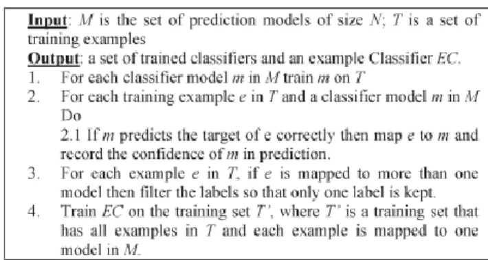
At first, all classifiers are trained on the training set T. The output of the training process is N -trained classifiers. During the mapping stage, each training example e in T is
mapped to one or more classifiers that succeed to predict its target. For example, in Fig. 3, t1 is mapped to classifier C2, while t3 is mapped to the set of classifiers C1, C2. The mapped training set
T_ undergoes a filtering process in which each example is mapped to only one classifier according to the confidence strength of the classifiers. For example, after filtering stage, t3 in
T_ is mapped to C1 rather than C1, C2 because
C2 predicts t3 correctly with higher probability, for instance. In case the models have equivalent prediction confidences, one model is selected randomly. Finally, the filtered data set FT is used to train the EC as the final output.
In this paper, we generate N orders of Markov models, namely, first, second, Nth-order Markov models, by applying sliding windows on the
training set T. These prediction models represent a repository that can be used in prediction. Next, we map each training example in T to one or more orders of Markov models.[4]
In this paper, we generate N orders of Markov models, namely, first, second, . . ., Nth-order Markov models, by applying sliding windows on the training set T. Fig 2 .These prediction models represent a repository that can be used in prediction. Next, we map each training example in
T to one or more orders of Markov models. For example, in Fig. 1, training example t3 : (P1, P3, P5) is mapped to two classifier IDs, namely, C1 (first-order Markov model) and C2 (second-order Markov model). After that, filtering/pruning process is conducted in which each example is mapped to only one classifier. In our experiments, we choose the classifier that predicts correctly with the highest probability.
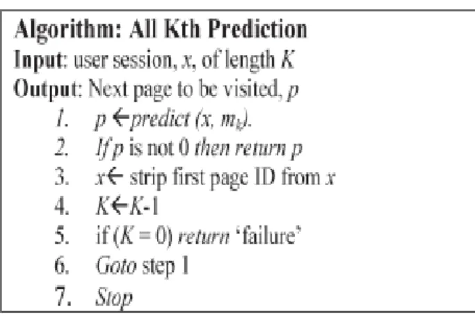
Fig 2. All kth prediction algorithm steps
B.Prediction Setup
Given a testing session (t) of length L, we conduct prediction using the (L − 1)-gram Markov model and obtain the prediction to evaluate the accuracy of the model. Recall that the last page of t is the final outcome that we will evaluate the correctness of the mode against; hence, we use (L − 1)-
gram. In case t is longer than the highest N-gram used in the experiment, we apply a sliding window of size L on t. For example, suppose t =
83 and p2, p3, p4, p5. Fig 3 shows the prediction
setup for 2 tier framework training process.[4]
Fig 3: Two tier framework training process
C. Ranking in Prediction Resolution
Once prediction models are built, we test these models against new examples. However, in many cases, a prediction model might give several outcomes, each with different support/probability. Note that resolving the prediction to only
the most probable target page would make the prediction accuracy very low because the accuracy can be computed as follows:
accuracy = - p ∈ pages ,dist(p) × pred(p)
where dist(p) is the target distribution of page p
and pred(p) is the target prediction accuracy of page p. For example, given a Web site of two pages with the following target distribution
and accuracy: dist(p1) = 0.4, dist(p2) = 0.6,
pred(p1) =0.65, and pred(p2) = 0.35, by (8), the accuracy of this Web site is 47%. Note that there are two factors that influence accuracy negatively in (8): 1) the low distribution of pages and 2) the higher interleaving targets of sessions, i.e., same session has more than one target. Unfortunately, in case of Web sites of large number of pages, these two factors affect accuracy negatively. Therefore, the prediction accuracy in Web
navigation is generally low.[4]
V. EXPERIMENTAL RESULTS
We first give a solution architecture diagram for the above. We first take the User’s input file which may be in excel format. He uploads the file in the application. The application runs and gives
the user the predicted output. Fig 4 shows the detailed architecture setup.
SOLUTION ARCHITECTURE DIAGRAM
In the first Step user enters the geospatial data input. The markov algorithm in analyzed and states are printed. The graphs etc are drawn. The user gets the predicted output. Use of java, jsp is done for the analysis.
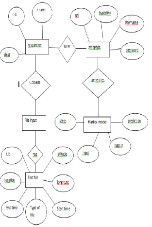
ER DIAGRAM FOR THE SYSTEM
VI. IMPLEMENTATION
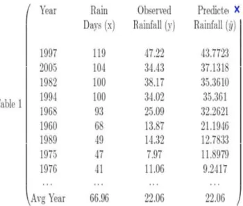
We use java, jsp for the implementation of this system. The researcher who is the main user of the system logins into the system and uploads his file. The web page then performs markov algorithm analyzes the data performs the analysis, tests, predicts the data accordingly. The given input data here is tested for the same and the rainfall data taken here is from period (1960-1997)
Fig 1 shows the login page of the system. New user must sign up if he has not registered. Only research scholors can use this application
Fig 1 User login page
Fig 2 shows the user upload page where the user uploads his excel sheet
Fig 2 Excel sheet upload
85 Fig 3: Experimental results using the tested sets
VII. CONCLUSION
The explosive growth of Geospatial data and widespread use of spatial databases emphasize the need for the automated discovery of spatial knowledge. GeoSpatial data mining is the process of discovering interesting and previously unknown, but potentially useful patterns from spatial databases. The complexity of spatial data and intrinsic spatial relationships limit the usefulness of conventional data mining techniques for extracting spatial patterns. Efficient tools for extracting information from geo-spatial data are crucial to organizations which make decisions based on large spatial datasets.
GeoSpatial data mining is a young and promising research domain. It is a potentially rich resource for spatial decision making and intelligent spatial analysis. More and more methods have been used to spatial data mining, including rough set, support vector machine, Markov Random Field, decision tree etc. GeoSpatial data mining should be combined with statistical and pattern analysis, spatial reasoning to create spatial decision support system and intelligent spatial information system.
VIII. REFERENCES
[1] By Jean-francFlorence, El Ghali Lazrak, Marc Catherine ,Annabelle Thibessard ,Pierre Leblond ,Using Markov Models to Mine Temporal and Spatial Data
[2]Campbell ,Alex, B.Pham, Y_C Tian,(Dept of CSE, Vanderbilt University,Nashville), A framework for Spatio-Temporal Data Analysis and Hypothesis Exploration,Survey Paper Year: April,1999.
[3]Shashi Shekhar, Senior Member, IEEE, Paul R. Schrater, Ranga R. Vatsavai, Weili Wu, Member, IEEE,, and Sanjay Chawla, Spatial Contextual Classification and Prediction Models for Mining Geospatial Data, Year of Publication:2002
[4] By Mamoun A. Awad and Issa Khalil ,
Prediction of User’s Web-Browsing Behavior: Application of Markov Model , 2012
[5] C. Y. Lin, M. Wu, J. A. Bloom, I. J. Cox, and M. Miller, ―Rotation, scale, and translation resilient public watermarking for images,‖
IEEE Trans. Image Process., vol. 10, no. 5, pp. 767-782, May 2001.
[6] M Levene and G Loizou, ―Computing the entropy Of User Navigation in the Web”, Int J Inf. Technol. Decision Making, vol 2,no3, pp.459-476,2003
Mr. P .Selvaraj is currently Assistant Professor at SRM University, Chennai. He is currently
pursuing Ph.d in Cognitive Networks. His area of interests include artificial intelligence, data mining, pattern recognition, Neural Networks etc.